Central Rockies (CR) Variant Overview of the Forest Vegetation Simulator - April 2023
←
→
Page content transcription
If your browser does not render page correctly, please read the page content below
Central Rockies (CR) Variant Overview of
the Forest Vegetation Simulator
April 2023
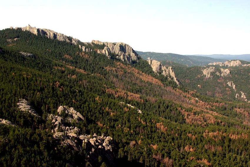
Harney Peak, Black Hills National Forest
(Blaine Cook, FS-R2)Central Rockies (CR) Variant Overview of
the Forest Vegetation Simulator
Authors and Contributors:
The FVS staff has maintained model documentation for this variant in the form of a variant
overview since its release in 1990. The original author was Gary Dixon. In 2008, the previous
document was replaced with this updated variant overview. Gary Dixon, Christopher Dixon,
Robert Havis, Chad Keyser, Stephanie Rebain, Erin Smith-Mateja, and Don Vandendriesche
were involved with this major update. Don Vandendriesche cross-checked information
contained in this variant overview with the FVS source code. In 2009, Gary Dixon, expanded the
species list and made significant updates to this variant overview.
FVS Staff. 2008 (revised April 3, 2023). Central Rockies (CR) Variant Overview – Forest
Vegetation Simulator. Internal Rep. Fort Collins, CO: U. S. Department of Agriculture, Forest
Service, Forest Management Service Center. 81p.
iiTable of Contents
Authors and Contributors: ..................................................................................................... ii
1.0 Introduction .................................................................................................................... 1
2.0 Geographic Range ............................................................................................................ 3
3.0 Control Variables ............................................................................................................. 4
3.0.1 Model Types ................................................................................................................................................4
3.1 Location Codes ....................................................................................................................................................4
3.2 Species Codes......................................................................................................................................................7
3.3 Habitat Type, Plant Association, and Ecological Unit Codes ...............................................................................9
3.4 Site Index ............................................................................................................................................................9
3.5 Maximum Density .............................................................................................................................................11
4.0 Growth Relationships .................................................................................................... 13
4.1 Height-Diameter Relationships .........................................................................................................................13
4.2 Bark Ratio Relationships ...................................................................................................................................15
4.3 Crown Ratio Relationships ................................................................................................................................16
4.3.1 Crown Ratio Dubbing ................................................................................................................................16
4.3.2 Crown Ratio Change ..................................................................................................................................19
4.3.3 Crown Ratio for Newly Established Trees .................................................................................................19
4.4 Crown Width Relationships ..............................................................................................................................19
4.5 Crown Competition Factor ................................................................................................................................23
4.6 Small Tree Growth Relationships ......................................................................................................................25
4.6.1 Small Tree Height Growth .........................................................................................................................25
4.6.2 Small Tree Diameter Growth.....................................................................................................................28
4.7 Large Tree Growth Relationships ......................................................................................................................29
4.7.1 Large Tree Diameter Growth ....................................................................................................................29
4.7.2 Large Tree Height Growth .........................................................................................................................34
5.0 Mortality Model ............................................................................................................ 47
6.0 Regeneration ................................................................................................................. 50
7.0 Volume .......................................................................................................................... 53
8.0 Fire and Fuels Extension (FFE-FVS).................................................................................. 57
9.0 Insect and Disease Extensions ........................................................................................ 58
10.0 Literature Cited ............................................................................................................ 59
iii11.0 Appendices .................................................................................................................. 63
11.1 Appendix A: Plant Association Codes for Region 2 Forests.............................................................................63
11.2 Appendix B: Plant Association Codes for Region 3 Forests .............................................................................73
ivQuick Guide to Default Settings
Parameter or Attribute Default Setting
Number of Projection Cycles 1 (10 if using FVS GUI)
Projection Cycle Length 10 years
Location Code (National Forest)
SM – Southwestern Mixed Conifers
(Region 2/Region 3) 213 – San Juan / 303 – Cibola
SP – Southwestern Ponderosa Pine
(Region 2/Region 3) 213 – San Juan / 303 – Cibola
BP – Black Hills Ponderosa Pine 203 – Black Hills
SF – Spruce-fir 206 – Medicine Bow – Routt
LP – Lodgepole Pine 206 – Medicine Bow – Routt
If model type is not set 303 – Cibola, model type set to SP
Model Type location code specific
Slope 5 percent
Aspect 0 (no meaningful aspect)
Elevation
SM – Southwestern Mixed Conifers 88 (8800 feet)
SP – Southwestern Ponderosa Pine 88 (8800 feet)
BP – Black Hills Ponderosa Pine 55 (5500 feet)
SF – Spruce-fir 90 (9000 feet)
LP – Lodgepole Pine 90 (9000 feet)
Latitude / Longitude Latitude Longitude
SM – Southwestern Mixed Conifers 38 107
SP – Southwestern Ponderosa Pine 38 107
BP – Black Hills Ponderosa Pine 44 107
SF – Spruce-fir; LP – Lodgepole Pine 40 107
Site Species
SM – Southwestern Mixed Conifers DF
SP – Southwestern Ponderosa Pine PP
BP – Black Hills Ponderosa Pine PP
SF – Spruce-fir ES
LP – Lodgepole Pine LP
Site Index
SM – Southwestern Mixed Conifers 70 feet (breast height age; 100 years)
SP – Southwestern Ponderosa Pine 70 feet (breast height age; 100 years)
BP – Black Hills Ponderosa Pine 57 feet (total age; 100 years)
SF – Spruce-fir 75 feet (breast height age; 100 years)
LP – Lodgepole Pine 65 feet (total age; 100 years)
Maximum Stand Density Index Species specific
vParameter or Attribute Default Setting
Maximum Basal Area Based on maximum stand density index
Volume Equations National Volume Estimator Library
Merchantable Cubic Foot Volume Specifications:
Minimum DBH / Top Diameter Hardwoods Softwoods
SM – Southwestern Mixed Conifers
SP – Southwestern Ponderosa Pine
SF – Spruce-fir
LP – Lodgepole Pine 5.0 / 4.0 inches 5.0 / 4.0 inches
BP – Black Hills Ponderosa Pine 9.0 / 6.0 inches 9.0 / 6.0 inches
Stump Height 1.0 foot 1.0 foot
Merchantable Board Foot Volume Specifications:
Minimum DBH / Top Diameter Hardwoods Softwoods
Region 2 Forests using these model types:
SM – Southwestern Mixed Conifers
SP – Southwestern Ponderosa Pine
SF – Spruce-fir
LP – Lodgepole Pine 7.0 / 6.0 inches 7.0 / 6.0 inches
Region 3 Forests using these model types:
SM – Southwestern Mixed Conifers
SP – Southwestern Ponderosa Pine
SF – Spruce-fir
LP – Lodgepole Pine 9.0 / 6.0 inches 9.0 / 6.0 inches
BP – Black Hills Ponderosa Pine 9.0 / 6.0 inches 9.0 / 6.0 inches
Stump Height 1.0 foot 1.0 foot
Sampling Design:
Large Trees (variable radius plot) 40 BAF
Small Trees (fixed radius plot) 1/300th acre
Breakpoint DBH 5.0 inches
vi1.0 Introduction
The Forest Vegetation Simulator (FVS) is an individual tree, distance independent growth and
yield model with linkable modules called extensions, which simulate various insect and
pathogen impacts, fire effects, fuel loading, snag dynamics, and development of understory
tree vegetation. FVS can simulate a wide variety of forest types, stand structures, and pure or
mixed species stands.
New “variants” of the FVS model are created by imbedding new tree growth, mortality, and
volume equations for a particular geographic area into the FVS framework. Geographic variants
of FVS have been developed for most of the forested lands in the United States.
The Central Rockies (CR) variant of FVS was developed in 1990. It was based on growth
equations and relationships from the GENGYM model (Edminster, Mowrer, Mathiasen, et. al.
1991). Although GENGYM is a diameter class model, and FVS is an individual tree model, results
produced with FVS were consistent with those produced by GENGYM. While general model
upgrades, enhancements, and error fixes, were made to the code since 1990, the variant
essentially remained the same as when it was developed.
In late 1998, staff at the Forest Management Service Center began a major overhaul of the
variant to correct known deficiencies and quirks, take advantage of advances in FVS technology,
incorporate additional data into certain model relationships, and improve default values and
surrogate species assignments. In addition, the model was expanded to include 24 species and
allow all National Forests within the geographic range of the model to access all the imbedded
model types.
In 2009 the variant was expanded from 24 species to 38 species. The juniper species group was
dropped and in its place was added the individual juniper species: Utah juniper, alligator
juniper, Rocky Mountain juniper, oneseed juniper, and eastern redcedar. These five individual
species all use the growth equations that were originally used for the juniper species group in
the 24 species version of the model. Similarly, the cottonwood species group was dropped and
in its place was added the individual cottonwood species: narrowleaf cottonwood and plains
cottonwood. Both of these individual species use the growth equations that were originally
used for the cottonwood species group. The oak species group was also dropped and in its
place was added the individual oak species: Gambel oak, Arizona white oak, Emory oak, bur
oak, and silverleaf oak. All five oak species uses the growth equations that were originally used
for the oak species group. Paper birch was added and uses growth equations for quaking aspen.
Chihuahuan pine was added and uses growth equations for ponderosa pine. Singleleaf pinyon,
border pinyon, and Arizona twoneedle pinyon were added and use growth equations for
common twoneedle pinyon.
To fully understand how to use this variant, users should also consult the following publication:
• Essential FVS: A User’s Guide to the Forest Vegetation Simulator (Dixon 2002)
1This publication may be downloaded from the Forest Management Service Center (FMSC),
Forest Service website. Other FVS publications may be needed if one is using an extension that
simulates the effects of fire, insects, or diseases.
22.0 Geographic Range
The CR variant was fit to data representing forest types in represented in the Wyoming, South
Dakota, Colorado, New Mexico, and Arizona. Data used in initial model development came from
growth samples from National Forests in these states.
The CR variant’s original range covered all forested land in Forest Service Regions 2 and 3. This
range extended from the northern border of Wyoming and Black Hills of South Dakota, down
through Colorado and western Nebraska, and into Arizona and New Mexico. The suggested
geographic range of use for the CR variant is shown in figure 2.0.1.
Figure 2.0.1 Suggested geographic range of use for the CR variant.
33.0 Control Variables
FVS users need to specify certain variables used by the CR variant to control a simulation. These
are entered in parameter fields on various FVS keywords available in the FVS interface or they
are read from an FVS input database using the Database Extension.
3.0.1 Model Types
The CR variant contains five different model types as shown in table 3.0.1.1. Model type may be
entered directly or if missing or an incorrect value is entered, then the default model type is
determined from the forest location code. The default model type by forest location code is
shown in table 3.1.1.
Some equations, for some species, are different depending on which model type is selected.
For example, ponderosa pine growth relationships are different if “Black Hills Ponderosa Pine”
is selected as the model type, as opposed to Southwestern Ponderosa Pine. For other species,
such as Douglas-fir, the growth equations are the same in all model types. The abbreviation
shown in the second column of table 3.0.1.1 is used to identify the model type and in labeling
some FVS output files.
Table 3.0.1.1 Model types used in the CR variant.
Model Type Output Abbreviation Description
1 SM Southwestern Mixed Conifers
2 SP Southwestern Ponderosa Pine
3 BP Black Hills Ponderosa Pine
4 SF Spruce-fir
5 LP Lodgepole Pine
3.1 Location Codes
The location code is a 3- or 4-digit code where, in general, the first digit of the code represents
the Forest Service Region Number, and the last two digits represent the Forest Number within
that region. In some cases, a location code beginning with a “7” or “8” is used to indicate an
administrative boundary that doesn’t use a Forest Service Region number (for example, other
federal agencies, state agencies, or other lands).
If the location code is missing or incorrect, the CR variant uses a default code depending on the
model type. If the model type is also missing or incorrect, or if the model type is 1 or 2, the
default forest is 303 (Cibola National Forest); if model type 3 is specified, the default forest
code is 203 (Black Hills National Forest); and if model types 4 or 5 is specified, the default forest
code is 206 (Medicine Bow – Routt National Forest). Location codes recognized in the CR
variant are shown in tables 3.1.1 and 3.1.2.
Table 3.1.1 Location codes and default model types used by the CR variant.
Forest Code National Forest Default Model Type
202 Bighorn Lodgepole Pine
4Forest Code National Forest Default Model Type
203 Black Hills Black Hills Ponderosa Pine
Grand Mesa, Uncompahgre,
204 Gunnison Spruce-fir
206 Medicine Bow - Routt Lodgepole Pine
207 Nebraska Black Hills Ponderosa Pine
209 Rio Grande Spruce-fir
210 Arapaho, Roosevelt Lodgepole Pine
212 Pike, San Isabel Spruce-fir
213 San Juan Spruce-fir
214 Shoshone Lodgepole Pine
215 White River Spruce-fir
301 Apache-Sitgreaves Southwestern Ponderosa Pine
302 Carson Southwestern Ponderosa Pine
303 Cibola Southwestern Ponderosa Pine
304 Coconino Southwestern Ponderosa Pine
305 Coronado Southwestern Ponderosa Pine
306 Gila Southwestern Ponderosa Pine
307 Kaibab Southwestern Ponderosa Pine
308 Lincoln Southwestern Ponderosa Pine
309 Prescott Southwestern Ponderosa Pine
310 Sante Fe Southwestern Ponderosa Pine
312 Tonto Southwestern Ponderosa Pine
201 Arapahoe (mapped to 210) Lodgepole Pine
205 Gunnison (mapped to 204) Spruce-fir
208 Pike (mapped to 212) Spruce-fir
211 Routt (mapped to 206) Lodgepole Pine
224 Grand Mesa (mapped to 204) Spruce-fir
311 Sitgreaves (mapped to 301) Southwestern Ponderosa Pina
Table 3.1.2 Bureau of Indian Affairs reservation codes used in the CR variant.
Location Code Location
7101 Cheyenne River Reservation (mapped to 203)
7104 Pine Ridge Reservation (mapped to 203)
7105 Rosebud Indian Reservation (mapped to 203)
7106 Yankton Reservation (mapped to 203)
7108 Standing Rock Reservation (mapped to 203)
7111 Santee Reservation (mapped to 207)
7113 Crow Creek Reservation (mapped to 203)
7114 Lower Brule Reservation (mapped to 203)
7206 Cheyenne-Arapaho Otsa (mapped to 310)
7207 Kiowa-Comanche-Apache-Fort Sill Apache Otsa (mapped to 310)
5Location Code Location
Kiowa-Comanche-Apache-Ft Sill-Apache/Caddo-Wichita-
7208 Delawarejoint-Use Otsa (mapped to 310)
7209 Caddo-Wichita-Delaware Otsa (mapped to 310)
7210 Kaw Otsa (mapped to 310)
7211 Otoe-Missouria Otsa (mapped to 310)
7213 Ponca Otsa (mapped to 310)
7214 Tonkawa Otsa (mapped to 310)
7217 Kickapoo (Tx/Mx) (mapped to 308)
7302 Crow Reservation (mapped to 202)
7305 Northern Cheyenne Off-Reservationtrust Land (mapped to 203)
7306 Wind River Reservation (mapped to 214)
7601 Chickasaw Otsa (mapped to 310)
7609 Osage Reservation (mapped to 310)
7701 Colorado River Indian Reservation (mapped to 312)
7702 Fort Mojave Reservation (mapped to 312)
7703 Chemehuevi Reservation (mapped to 312)
7704 Fort Apache Reservation (mapped to 301)
7705 Tohono O'Odham Nation Reservation (mapped to 312)
7706 Fort Mcdowell Yavapai Nation Reservation (mapped to 312)
7707 Salt River Reservation (mapped to 312)
7708 Maricopa, (Ak Chin Indian Res (mapped to 312)
7709 Gila River Indian Reservation (mapped to 312)
7710 San Carlos Reservation (mapped to 305)
7718 Uintah And Ouray Reservation (mapped to 215)
7719 Cocopah Reservation (mapped to 312)
7720 Fort Yuma Indian Reservation (mapped to 312)
7724 Hopi Reservation (mapped to 301)
7725 Havasupai Reservation (mapped to 307)
7726 Hualapai Indian Reservation (mapped to 307)
7727 Yavapai-Prescott Reservation (mapped to 309)
7728 Kaibab Indian Reservation (mapped to 307)
7835 Timbi-Sha Shoshone Reservation (mapped to 312)
7847 Agua Caliente Indian Reservation (mapped to 312)
7848 Augustine Reservation (mapped to 312)
7859 Morongo Reservation (mapped to 312)
7901 Acoma Pueblo (mapped to 303)
7902 Pueblo De Cochiti (mapped to 310)
7903 Isleta Pueblo (mapped to 303)
7904 Jemez Pueblo (mapped to 310)
7905 Sandia Pueblo (mapped to 303)
7906 San Felipe Pueblo (mapped to 310)
6Location Code Location
7907 Santa Ana Pueblo (mapped to 310)
7908 Santo Domingo Pueblo (mapped to 310)
7909 Zia Pueblo (mapped to 310)
7910 Laguna Pueblo (mapped to 303)
7911 Nambe Pueblo (mapped to 310)
7912 Picuris Pueblo (mapped to 302)
7913 Pueblo Of Pojoaque (mapped to 310)
7914 San Ildefonso Pueblo (mapped to 310)
7915 Ohkay Owingeh (mapped to 302)
7916 Santa Clara Pueblo (mapped to 310)
7917 Taos Pueblo (mapped to 302)
7918 Tesuque Pueblo (mapped to 310)
7919 Southern Ute Reservation (mapped to 213)
7920 Ute Mountain Reservation (mapped to 213)
7921 Jicarilla Apache Nation Reservation (mapped to 302)
7922 Mescalero Reservation (mapped to 308)
7923 Fort Sill Apache Indian Reservation (mapped to 306)
7924 Zuni Reservation (mapped to 303)
7925 Ramah-Navajo (mapped to 303)
8001 Navajo Nation Reservation (mapped to 301)
3.2 Species Codes
The CR variant recognizes 36 species, plus two other composite species categories. You may use
FVS species codes, Forest Inventory and Analysis (FIA) species codes, or USDA Natural
Resources Conservation Service PLANTS symbols to represent these species in FVS input data.
Any valid western species code identifying species not recognized by the variant will be mapped
to a similar species in the variant. The species mapping crosswalk is available on the FVS
website variant documentation webpage. Any non-valid species code will default to the “other
hardwood” category.
Either the FVS sequence number or species code must be used to specify a species in FVS
keywords and Event Monitor functions. FIA codes or PLANTS symbols are only recognized
during data input and may not be used in FVS keywords. Table 3.2.1 shows the complete list of
species codes recognized by the EM variant.
When entering tree data, users should substitute diameter at root collar (DRC) for diameter at
breast height (DBH) for woodland species (pinyons, junipers, and oaks other than bur oak).
Table 3.2.1 Species codes used in the CR variant.
Species Species FIA PLANTS
Number Code Code Symbol Scientific Name1 Common Name1
1 AF 019 ABLA Abies lasiocarpa subalpine fir
7Species Species FIA PLANTS
Number Code Code Symbol Scientific Name1 Common Name1
Abies lasiocarpa var.
2 CB 018 ABLAA arizonica corkbark fir
3 DF 202 PSME Pseudotsuga menziesii Douglas-fir
4 GF 017 ABGR Abies grandis grand fir
5 WF 015 ABCO Abies concolor white fir
6 MH 264 TSME Tsuga mertensiana mountain hemlock
7 RC 242 THPL Thuja plicata western redcedar
8 WL 073 LAOC Larix occidentalis western larch
9 BC 102 PIAR Pinus aristata bristlecone pine
10 LM 113 PIFL2 Pinus flexilis limber pine
11 LP 108 PICO Pinus contorta lodgepole pine
12 PI 106 PIED Pinus edulis twoneedle pinyon
13 PP 122 PIPO Pinus ponderosa ponderosa pine
14 WB 101 PIAL Pinus albicaulis whitebark pine
southwestern white
15 SW 114 PIST3 Pinus strobiformis pine
16 UJ 065 JUOS Juniperus osteosperma Utah juniper
17 BS 096 PIPU Picea pungens blue spruce
18 ES 093 PIEN Picea engelmannii Engelmann spruce
19 WS 094 PIGL Picea glauca white spruce
20 AS 746 POTR5 Populus tremuloides quaking aspen
21 NC 749 POAN3 Populus angustifolia narrowleaf cottonwood
Populus deltoides ssp.
22 PW 745 PODEM monilifera plains cottonwood
23 GO 814 QUGA Quercus gambelii Gambel oak
24 AW 803 QUAR Quercus arizonica Arizona white oak
25 EM 810 QUEM Quercus emoryi Emory oak
26 BK 823 QUMA2 Quercus macrocarpa bur oak
27 SO 843 QUHY Quercus hypoleucoides silverleaf oak
28 PB 375 BEPA Betula papyrifera paper birch
29 AJ 063 JUDE2 Juniperus deppeana alligator juniper
30 RM 066 JUSC2 Juniperus scopulorum Rocky Mountain juniper
31 OJ 069 JUMO Juniperus monosperma oneseed juniper
32 ER 068 JUVI Juniperus virginiana eastern redcedar
33 PM 133 PIMO Pinus monophylla singleleaf pinyon
34 PD 134 PIDI3 Pinus discolor border pinyon
Pinus monophylla var. Arizona twoneedle
35 AZ 143 PIMOF fallax pinyon3
36 CI 118 PILE Pinus leiophylla Chihuahuan pine
37 OS 299 2TN other softwood2
8Species Species FIA PLANTS
Number Code Code Symbol Scientific Name1 Common Name1
38 OH 998 2TB other hardwood2
1Set based on the USDA Forest Service NRM TAXA lists and the USDA Plants database.
2Other categories use FIA codes and NRM TAXA codes that best match the other category.
3Common name is from FIA master species list, January, 1 2021.
3.3 Habitat Type, Plant Association, and Ecological Unit Codes
In the CR variant, plant association codes are used in the Fire and Fuels Extension (FFE) to set fuel
loading in cases where there are no trees in the first cycle. Codes recognized in the CR variant are
the NRIS Common Stand Exam codes (US Forest Service 2000). Valid codes are shown in
Appendices A and B. Region 2 codes originate from Johnson (1987), and Region 3 codes from
US Forest Service (1997). Users may enter the plant association code or the plant association
FVS sequence number on the STDINFO keyword, when entering stand information from a
database, or when using the SETSITE keyword without the PARMS option. If using the PARMS
option with the SETSITE keyword, users must use the FVS sequence number for the plant
association.
3.4 Site Index
Site index is used in the growth equations for the CR variant. When possible, users should enter
their own values instead of relying on the default values assigned by FVS. If site index
information is available, a single site index can be specified for the whole stand, a site index for
each individual species can be specified, or a combination of these can be entered. If the user
does not supply site index values, then default values will be used. When entering site index in
the CR variant, the sources shown in table 3.4.1 should be used if possible. Default values for
site species and site index, by model type, are shown in table 3.4.2.
When site index is not specified for a species, a relative site index value is calculated from the
site index of the site species using equations {3.4.1} and {3.4.2}. Minimum and Maximum site
indices used in equation {3.4.1} may be found in table 3.4.3. If the site index for the stand is
less than or equal to the lower site limit, it is set to the lower limit + 0.5 for the calculation of
RELSI. Similarly, if the site index for the stand is greater than the upper site limit, it is set to the
upper site limit for the calculation of RELSI.
{3.4.1} RELSI = (SIsite – SITELOsite) / (SITEHIsite – SITELOsite)
{3.4.2} SIi = SITELOi + RELSI * (SITEHIi – SITELOi)
where:
RELSI is the relative site index of the site species
SI is species site index
SITELO is the lower bound of the SI range for a species
SITEHI is the upper bound of the SI range for a species
site is the site species
9i is the species for which site index is to be calculated
Table 3.4.1 Recommended site index references for use with the CR variant.
Reference Ref
Model Type Species Age Age Type Reference
Edminster, Mathiasen, Olsen
SW Mixed Conifers DF 100 Breast Height 1991
SW Ponderosa Pine PP 100 Breast Height Minor 1964
BHills Ponderosa Pine PP 100 Total Meyer 1961
Spruce-fir ES / AF 100 Breast Height Alexander 1967
Alexander, Tackle, Dahms
Lodgepole Pine LP 100 Total 1967
Table 3.4.2 Default values for site species and site index, by model type, for the CR variant.
Model Type Site Species Site Index
SW Mixed Conifers DF 70
SW Ponderosa Pine PP 70
Black Hills Ponderosa Pine PP 57
Spruce-fir ES 75
Lodgepole Pine LP 65
Table 3.4.3 Default SITELO and SITEHI values for equation {3.4.1} in the CR variant.
Species
Code SITELO SITEHI
AF 40 105
CB 30 100
DF 40 120
GF 30 130
WF 40 105
MH 40 70
RC 20 125
WL 40 120
BC 20 60
LM 10 60
LP 30 95
PI 6 40
PP 30 100
WB 20 60
SW 30 130
UJ 6 30
BS 30 110
ES 40 120
WS 30 85
AS 20 100
NC 30 120
10Species
Code SITELO SITEHI
PW 30 120
GO 6 40
AW 6 40
EM 6 40
BK 6 40
SO 6 40
PB 20 100
AJ 6 30
RM 6 30
OJ 6 30
ER 6 30
PM 6 40
PD 6 40
AZ 6 40
CI 30 100
OS 30 95
OH 20 100
3.5 Maximum Density
Maximum stand density index (SDI) and maximum basal area (BA) are important variables in
determining density related mortality and crown ratio change. Maximum basal area is a stand
level metric that can be set using the BAMAX or SETSITE keywords. If not set by the user, a
default value is calculated from maximum stand SDI each projection cycle. Maximum stand
density index can be set for each species using the SDIMAX or SETSITE keywords. If not set by
the user, a default value is assigned as discussed below.
The default maximum SDI is set based on species or a user specified basal area maximum. If a
user specified basal area maximum is present, the maximum SDI for all species is computed
using equation {3.5.1}; otherwise, species SDI maximums are assigned from the SDI maximums
shown in table 3.5.1. Maximum stand density index at the stand level is a weighted average, by
basal area, of the individual species SDI maximums.
Stand SDI is calculated using the Zeide calculation method (Dixon 2002).
{3.5.1} SDIMAXi = BAMAX / (0.5454154 * SDIU)
where:
SDIMAXi is the species-specific SDI maximum
BAMAX is the user-specified stand basal area maximum
SDIU is the proportion of theoretical maximum density at which the stand reaches
actual maximum density (default 0.85, changed with the SDIMAX keyword)
Table 3.5.1 Default stand density index maximums by species in the CR variant.
11Species SDI
Code Maximum* Mapped to
AF 602
CB 423
DF 570
GF 562
WF 634
MH 687
RC 762
WL 423
BC 621 whitebark pine
LM 409
LP 679
PI 348
PP 446
WB 621
SW 529 eastern white pine
UJ 497
BS 620 Engelmann spruce
ES 620
WS 412
AS 562
NC 452 black cottonwood
PW 452 black cottonwood
GO 652
AW 403
EM 284
BK 423
SO 284 Emory oak
PB 466
AJ 395
RM 411
OJ 408
ER 354
PM 358
PD 348 twoneedle pinyon
AZ 358 singleleaf pinyon
CI 446 ponderosa pine
OS 348 twoneedle pinyon
OH 452 black cottonwood
*Source of SDI maximums is an unpublished analysis of FIA data by John Shaw.
124.0 Growth Relationships
This chapter describes the functional relationships used to fill in missing tree data and calculate
incremental growth. In FVS, trees are grown in either the small tree sub-model or the large tree
sub-model depending on the diameter.
4.1 Height-Diameter Relationships
Height-diameter relationships in FVS are primarily used to estimate tree heights missing in the
input data and occasionally to estimate diameter growth on trees smaller than a given
threshold diameter. In the CR variant, height-diameter relationships are a logistic functional
form, as shown in equation {4.1.1} (Wykoff, et.al 1982). The equation was fit to data of the
same species used to develop other FVS variants. Default coefficients for equation {4.1.1} are
shown are shown in table 4.1.1.
When heights are given in the input data for 3 or more trees of a given species, the value of B 1
in equation {4.1.1} for that species is recalculated from the input data and replaces the default
value shown in table 4.1.1. In the event that the calculated value is less than zero, the default is
used.
{4.1.2} Wykoff functional form
HT = 4.5 + exp(B1 + B2 / (DBH + 1.0))
where:
HT is tree height
DBH is tree diameter at breast height
B1 - B2 are species-specific coefficients shown in table 4.1.1
Table 4.1.1 Default coefficients for the height-diameter relationship equation in the CR
variant.
Species
Code B1 B2
AF 4.4717 -6.7387
CB 4.4717 -6.7387
DF 4.5879 -8.9277
GF 5.0271 -11.2168
WF 4.3008 -6.8139
MH 4.8740 -10.4050
RC 5.1631 -9.2566
WL 5.1631 -9.2566
BC 4.1920 -5.1651
LM 4.1920 -5.1651
LP 4.3767 -6.1281
PI 4.1920 -5.1651
13Species
Code B1 B2
PP 4.6024 -11.4693
WB 4.1920 -5.1651
SW 5.1999 -9.2672
UJ 4.1920 -5.1651
BS 4.5293 -7.7725
ES 4.5293 -7.7725
WS 4.5293 -7.7725
AS 4.4421 -6.5405
NC 4.4421 -6.5405
PW 4.4421 -6.5405
GO 4.1920 -5.1651
AW 4.1920 -5.1651
EM 4.1920 -5.1651
BK 4.1920 -5.1651
SO 4.1920 -5.1651
PB 4.4421 -6.5405
AJ 4.1920 -5.1651
RM 4.1920 -5.1651
OJ 4.1920 -5.1651
ER 4.1920 -5.1651
PM 4.1920 -5.1651
PD 4.1920 -5.1651
AZ 4.1920 -5.1651
CI 4.6024 -11.4693
OS 4.2597 -9.3949
OH 4.4421 -6.5405
For the Black Hills Ponderosa Pine model type, the default height-diameter relationships for all
species are shown in the equations {4.1.2} and {4.1.3}. Trees with a DBH greater than 0.5 inches
use equation {4.1.2} and trees with a DBH less than or equal to 0.5 inches use equation {4.1.3}.
{4.1.2} HT = 32.108633 * (SI^0.276926) * [(1 – exp(-0.057766*DBH))^ 1.0026686] + 4.5
{4.1.3} HT = DBH * [12.41173 + 0.04633 * SI – 0.000158 * SI^2]
where:
HT is tree height
DBH is tree diameter at breast height
SI is species site index
However, the calibrated logistic function is used for a given species when there are enough
observations to get a satisfactory estimate of the “a” parameter for that species.
144.2 Bark Ratio Relationships
Bark ratio estimates are used to convert between diameter outside bark and diameter inside
bark in various parts of the model. The equation is shown in equation {4.2.1} and coefficients
(b1 and b2) for this equation by species are shown in table 4.2.1.
{4.2.1} BRATIO = b1 + b2 * (1 / DBH)
Note: if a species has a b2 value equal to 0, then BRATIO = b1
where:
BRATIO is species-specific bark ratio (bounded to 0.80 < BRATIO < 0.99)
DBH is tree diameter at breast height (bounded to DBH > 1.0)
b1 - b2 are species-specific coefficients shown in table 4.2.1
Table 4.2.1 Default coefficients for the bark ratio equation {4.2.1} in the CR variant.
Species
Code Model Type b1 b2 Equation Source
AF all 0.890 0 PP from Wykoff, et. al. 1982
CB all 0.890 0 PP from Wykoff, et. al. 1982
DF all 0.867 0 Wykoff, et. al. 1982
GF all 0.890 0 PP from Wykoff, et. al. 1982
WF all 0.890 0 PP from Wykoff, et. al. 1982
MH all 0.9497 0 Wykoff, et. al. 1982
RC all 0.9497 0 Wykoff, et. al. 1982
WL all 0.87407 -0.185 Schmidt, et. al. 1976
BC all 0.9625 -0.1141 Uses LP equation
LM all 0.9625 -0.1141 Uses LP equation
LP all 0.9625 -0.1141 Myers 1964
PI SM, SP 0.8967 -0.4448 PP from Dolph PSW-368
PI BP, SF, LP 0.9002 -0.3089 Uses PP equation
PP SM, SP 0.8967 -0.4448 PP from Dolph PSW-368
PP BP, SF, LP 0.9002 -0.3089 Myers & Van Deusen 1958
WB all 0.9625 -0.1141 Uses LP equation
SW all 0.9643 0 Wykoff, et. al. 1982
UJ SM, SP 0.8967 -0.4448 PP from Dolph PSW-368
UJ BP, SF, LP 0.9002 -0.3089 Uses PP equation
BS all 0.9502 -0.2528 Uses ES equation
ES all 0.9502 -0.2528 Myers & Alexander 1972
WS all 0.9502 -0.2528 Uses ES equation
AS all 0.950 0 Utah FVS variant
NC all 0.892 -0.086 Edminster, et. al. 1977
PW all 0.892 -0.086 Edminster, et. al. 1977
GO 0.93789 -0.24096 Clark, et. al. 1991
15Species
Code Model Type b1 b2 Equation Source
AW 0.93789 -0.24096 Clark, et. al. 1991
EM 0.93789 -0.24096 Clark, et. al. 1991
BK 0.93789 -0.24096 Clark, et. al. 1991
SO 0.93789 -0.24096 Clark, et. al. 1991
PB 0.950 0 Uses AS equation
AJ SM, SP 0.8967 -0.4448 PP from Dolph PSW-368
AJ BP, SF, LP 0.9002 -0.3089 Uses PP equation
RM SM, SP 0.8967 -0.4448 PP from Dolph PSW-368
RM BP, SF, LP 0.9002 -0.3089 Uses PP equation
OJ SM, SP 0.8967 -0.4448 PP from Dolph PSW-368
OJ BP, SF, LP 0.9002 -0.3089 Uses PP equation
ER SM, SP 0.8967 -0.4448 PP from Dolph PSW-368
ER BP, SF, LP 0.9002 -0.3089 Uses PP equation
PM SM, SP 0.8967 -0.4448 PP from Dolph PSW-368
PM BP, SF, LP 0.9002 -0.3089 Uses PP equation
PD SM, SP 0.8967 -0.4448 PP from Dolph PSW-368
PD BP, SF, LP 0.9002 -0.3089 Uses PP equation
AZ SM, SP 0.8967 -0.4448 PP from Dolph PSW-368
AZ BP, SF, LP 0.9002 -0.3089 Uses PP equation
CI SM, SP 0.8967 -0.4448 PP from Dolph PSW-368
CI BP, SF, LP 0.9002 -0.3089 Uses PP equation
OS SM, SP 0.8967 -0.4448 PP from Dolph PSW-368
OS BP, SF, LP 0.9002 -0.3089 Uses PP equation
OH all 0.892 -0.086 Uses CO equation
* DBH is bounded between 1.0 and 19.0 for species using the PP equation (coefficients 0.9002
and -0.3089).
4.3 Crown Ratio Relationships
Crown ratio equations are used for three purposes in FVS: (1) to estimate tree crown ratios
missing from the input data for both live and dead trees; (2) to estimate change in crown ratio
from cycle to cycle for live trees; and (3) to estimate initial crown ratios for regenerating trees
established during a simulation.
4.3.1 Crown Ratio Dubbing
In the CR variant, all species except mountain hemlock, western redcedar, and western larch
use equations from GENGYM which predict crown length as a function of tree and stand
attributes using equation {4.3.1.1}. Coefficients for this equation are shown in table 4.3.1.1.
Crown length is then converted to crown ratio by dividing crown length by total tree height as
shown in equation {4.3.1.2}.
{4.3.1.1} CL = a0 + (a1 * HT) + (a2 * DBH) + (a3 * BA) + (a4 * BAU)
16{4.3.1.2} CR = CL / HT
where:
CL is tree crown length
HT is tree height
DBH is tree diameter at breast height
BA is total stand basal area
BAU is total basal area in trees above the diameter class of the subject tree
CR is predicted crown ratio expressed as a proportion at the end of the cycle
a0 – a4 are species-specific coefficients shown in table 4.3.1.1
Table 4.3.1.1 Default coefficients to predict crown length for equation {4.3.1.1} in the CR
variant.
Species
Code Model Type a0 a1 a2 a3 a4
AF SM, SP 0.50706 0.73070 0 0 0
AF BP, SF, LP 0.36135 0.57085 0 0 0
CB SM, SP 0.50706 0.73070 0 0 0
CB BP, SF, LP 0.36135 0.57085 0 0 0
DF ALL 6.47479 0.50703 0.54482 -0.03326 0
GF ALL 6.22959 0.67587 0 -0.03098 0
WF ALL 6.22959 0.67587 0 -0.03098 0
MH *
RC *
WL *
BC ALL -0.59373 0.67703 0 0 0
LM ALL -0.59373 0.67703 0 0 0
LP ALL 5.00215 0.06334 0.88236 0 -0.03821
PI ALL -0.59373 0.67703 0 0 0
PP SM 5.63367 0.56252 0 -0.06411 0
PP SP 4.35671 0.32549 0.84714 -0.03802 0
PP BP, SF, LP 3.49178 0.17421 0.80767 -0.03272 0
WB ALL -0.59373 0.67703 0 0 0
SW ALL 3.03832 0.65587 0 -0.01792 0
UJ ALL -0.59373 0.67703 0 0 0
BS ALL 3.61635 0.61547 0.93639 -0.02360 0
ES SM, SP 1.05857 0.68442 0 0 0
ES BP, SF, LP 3.22244 0.44315 0.44755 0 0
WS ALL 0.15768 0.74697 0 0 0
AS ALL 5.17281 0.32552 0 -0.01675 0
NC ALL 5.17281 0.32552 0 -0.01675 0
PW ALL 5.17281 0.32552 0 -0.01675 0
GO ALL -0.59373 0.67703 0 0 0
17Species
Code Model Type a0 a1 a2 a3 a4
AW ALL -0.59373 0.67703 0 0 0
EM ALL -0.59373 0.67703 0 0 0
BK ALL -0.59373 0.67703 0 0 0
SO ALL -0.59373 0.67703 0 0 0
PB ALL 5.17281 0.32552 0 -0.01675 0
AJ ALL -0.59373 0.67703 0 0 0
RM ALL -0.59373 0.67703 0 0 0
OJ ALL -0.59373 0.67703 0 0 0
ER ALL -0.59373 0.67703 0 0 0
PM ALL -0.59373 0.67703 0 0 0
PD ALL -0.59373 0.67703 0 0 0
AZ ALL -0.59373 0.67703 0 0 0
CI SM 5.63367 0.56252 0 -0.06411 0
CI SP 4.35671 0.32549 0.84714 -0.03802 0
CI BP, SF, LP 3.49178 0.17421 0.80767 -0.03272 0
OS ALL -0.59373 0.67703 0 0 0
OH ALL 5.17281 0.32552 0 -0.01675 0
*Crown ratio equations for MH, RC, and WL are described below
The remaining three species use equations from other variants that predict crown ratio directly.
The equation for mountain hemlock is given in equation {4.3.1.3}. This equation is from the
North Idaho (NI) variant for Bitterroot National Forest and habitat type set to 710. The equation
for western red cedar is shown in equation {4.3.1.4}. This equation is from the NI variant with
habitat type set to 550. The equation for western larch is shown in equation {4.3.1.5}. This
equation is also from the NI variant for Bitterroot National Forest and habitat type set to 260.
{4.3.1.3} CR = 0.3450 – (0.00264 * BA) + (0.00000512 * CCF^2) – (0.25138 * ln(HT)) + (0.05140 * ln(PCT))
{4.3.1.4} CR = -1.6053 + (0.17479 * ln(BA)) – (0.00183 * CCF) – (0.00560 * DBH) + (0.11050 * ln(PCT))
{4.3.1.5} CR = 0.03441 – (0.00204 * BAT) + (0.30066 * ln(DBH)) – (0.59302 * ln(HT))
where:
CR is predicted crown ratio expressed as a proportion at the end of the cycle
BA is total stand basal area
CCF is stand crown competition factor
HT is tree height at the beginning of the cycle
PCT is the subject tree’s percentile in the basal area distribution of the stand
DBH is tree diameter at breast height
BAT is total stand basal area (subject to restrictions)
BAT is subject to the following restrictions:
Southwestern Mixed Conifers model type:
BAT > 1.0
If BAT is less than 65, then BAL is set to 0.
18Southwestern Ponderosa Pine model type:
BAT > 21
Black Hills Ponderosa Pine and Spruce-Fir model types:
BAT > 5
Lodgepole pine model type:
BAT > 14
4.3.2 Crown Ratio Change
Crown ratio change is estimated after growth, mortality and regeneration are estimated during
a projection cycle. Crown ratio change is the difference between the crown ratio at the
beginning of the cycle and the predicted crown ratio at the end of the cycle. Crown ratio
predicted at the end of the projection cycle is estimated for live tree records using the
equations outlined above. Once crown ratio is predicted, it is bounded to a change of no more
than 1% per year, and to no more than the potential change in crown ratio if all the height
growth contributed to the crown change during the cycle.
4.3.3 Crown Ratio for Newly Established Trees
Crown ratios for newly established trees during regeneration are estimated using equation
{4.3.3.1}. A random component is added in equation {4.3.3.1} to ensure that not all newly
established trees are assigned exactly the same crown ratio.
{4.3.3.1} CR = 0.89722 – 0.0000461 * PCCF + RAN
where:
CR is crown ratio expressed as a proportion (bounded to 0.2 < CR < 0.9)
PCCF is crown competition factor on the inventory point where the tree is established
RAN is a small random component
4.4 Crown Width Relationships
The CR variant calculates the maximum crown width for each individual tree based on
individual tree and stand attributes. Crown width for each tree is reported in the tree list
output table and used for percent canopy cover (PCC) calculations in the model. Crown width is
calculated using equations {4.4.1} – {4.4.5}, and coefficients for these equations are shown in
table 4.4.1. The minimum diameter and bounds for certain data values are given in table 4.4.2.
Equation numbers in table 4.4.1 are given with the first three digits representing the FIA species
code and the last two digits representing the equation source.
{4.4.1} Bechtold (2004); Equation 01
DBH > MinD: CW = a1 + (a2 * DBH) + (a3 * DBH^2)
DBH < MinD: CW = [a1 + (a2 * MinD) * (a3 * MinD^2)] * (DBH / MinD)
19{4.4.2} Bechtold (2004); Equation 02
DBH > MinD: CW = a1 + (a2 * DBH) + (a3 * DBH^2) + (a4 * CR) + (a5 * BA) + (a6 * HI)
DBH < MinD: CW = [a1 + (a2 * MinD) + (a3 * MinD^2) + (a4 * CR) + (a5 * BA) + (a6 * HI)] * (DBH
/ MinD)
{4.4.3} Crookston (2003); Equation 03 (used only for Mountain Hemlock)
HT < 5.0: CW = [0.8 * HT * MAX(0.5, CR * 0.01)] * [1 - (HT - 5) * 0.1] * a1 * DBH^a2 * HT^a3 *
CL^a4 * (HT-5) * 0.1
5.0 < HT < 15.0: CW = 0.8 * HT * MAX(0.5, CR * 0.01)
HT > 15.0: CW = a1 * (DBH^a2) * (HT^a3) * (CL^a4)
{4.4.4} Crookston (2003); Equation 03
DBH > MinD: CW = [a1 * exp[a2 + (a3 * ln(CL)) + (a4 * ln(DBH)) + (a5 * ln(HT)) + (a6 * ln(BA))]]
DBH < MinD: CW = [a1 * exp[a2 + (a3 * ln(CL)) + (a4 * ln(MinD)) + (a5 * ln(HT)) + (a6 * ln(BA))]]
* (DBH / MinD)
{4.4.5} Crookston (2005); Equation 05
DBH > MinD: CW = (a1 * BF) * DBH^a2 * HT^a3 * CL^a4 * (BA + 1.0)^a5 * (exp(EL))^a6
DBH < MinD: CW = [(a1 * BF) * MinD^a2 * HT^a3 * CL^a4 * (BA + 1.0)^a5 * (exp(EL))^a6] *
(DBH / MinD)
where:
BF is a species-specific coefficient based on forest code (BF = 1.0 in the CR variant)
CW is tree maximum crown width
CL is tree crown length
DBH is tree diameter at breast height
HT is tree height
BA is total stand basal area
EL is stand elevation in hundreds of feet
MinD is the minimum diameter
HI is the Hopkins Index
HI = (ELEVATION - 5449) / 100) * 1.0 + (LATITUDE - 42.16) * 4.0 + (-116.39 -
LONGITUDE) * 1.25
a1 – a6 are species-specific coefficients shown in table 4.4.1
Table 4.4.1 Default coefficients for crown width equations {4.4.1} – {4.4.5} in the CR variant.
Species Equation
Code Number* a1 a2 a3 a4 a5 a6
AF 01905 5.8827 0.51479 -0.21501 0.17916 0.03277 -0.00828
CB 01801 6.073 0.3756 0 0 0 0
20Species Equation
Code Number* a1 a2 a3 a4 a5 a6
DF 20205 6.0227 0.54361 -0.20669 0.20395 -0.00644 -0.00378
GF 01703 1.0303 1.14079 0.20904 0.38787 0 0
WF 01505 5.0312 0.53680 -0.18957 0.16199 0.04385 -0.00651
MH 26403 6.90396 0.55645 -0.28509 0.20430 0 0
RC 24205 6.2382 0.29517 -0.10673 0.23219 0.05341 -0.00787
WL 07303 1.02478 0.99889 0.19422 0.59423 -0.09078 -0.02341
BC 10201 7.4251 0.8991 0 0 0 0
LM 11301 4.0181 0.8528 0 0 0 0
LP 10805 6.6941 0.81980 -0.36992 0.17722 -0.01202 -0.00882
PI 10602 -5.4647 1.9660 0 -0.0395 0.0427 -0.0259
PP 12205 4.7762 0.74126 -0.28734 0.17137 -0.00602 -0.00209
WB 10105 2.2354 0.66680 -0.11658 0.16927 0 0
SW 11905 5.3822 0.57896 -0.19579 0.14875 0 -0.00685
UJ 06602 -4.1599 1.3528 0 -0.0233 0.0633 -0.0423
BS 09305 6.7575 0.55048 -0.25204 0.19002 0 -0.00313
ES 09305 6.7575 0.55048 -0.25204 0.19002 0 -0.00313
WS 09305 6.7575 0.55048 -0.25204 0.19002 0 -0.00313
AS 74605 4.7961 0.64167 -0.18695 0.18581 0 0
NC 74902 4.1687 1.5355 0 0 0 0.1275
PW 74902 4.1687 1.5355 0 0 0 0.1275
GO 81402 0.3309 0.8918 0 0 0.0510 0
AW 81402 0.3309 0.8918 0 0 0.0510 0
EM 81402 0.3309 0.8918 0 0 0.0510 0
BK 81402 0.3309 0.8918 0 0 0.0510 0
SO 81402 0.3309 0.8918 0 0 0.0510 0
PB 74605 4.7961 0.64167 -0.18695 0.18581 0 0
AJ 06602 -4.1599 1.3528 0 -0.0233 0.0633 -0.0423
RM 06602 -4.1599 1.3528 0 -0.0233 0.0633 -0.0423
OJ 06602 -4.1599 1.3528 0 -0.0233 0.0633 -0.0423
ER 06602 -4.1599 1.3528 0 -0.0233 0.0633 -0.0423
PM 10602 -5.4647 1.9660 0 -0.0395 0.0427 -0.0259
PD 10602 -5.4647 1.9660 0 -0.0395 0.0427 -0.0259
AZ 10602 -5.4647 1.9660 0 -0.0395 0.0427 -0.0259
CI 12205 4.7762 0.74126 -0.28734 0.17137 -0.00602 -0.00209
OS 12205 4.7762 0.74126 -0.28734 0.17137 -0.00602 -0.00209
OH 74902 4.1687 1.5355 0 0 0 0.1275
*Equation number is a combination of the species FIA code (###) and source (##).
Table 4.4.2 Default MinD values and data bounds for equations {4.4.1} – {4.4.5} in the CR
variant.
21Species Equation
Code Number* MinD EL min EL max HI min HI max CW max
AF 01905 1.0 10 85 n/a n/a 30
CB 01801 5.0 n/a n/a n/a n/a 15
DF 20205 1.0 1 75 n/a n/a 80
GF 01703 1.0 n/a n/a n/a n/a 40
WF 01505 1.0 2 75 n/a n/a 35
MH 26403 n/a n/a n/a n/a n/a 45
RC 24205 1.0 1 72 n/a n/a 45
WL 07303 1.0 n/a n/a n/a n/a 40
BC 10201 5.0 n/a n/a n/a n/a 25
LM 11301 5.0 n/a n/a n/a n/a 25
LP 10805 1.0 1 79 n/a n/a 40
PI 10602 5.0 n/a n/a -40 11 25
PP 12205 1.0 13 75 n/a n/a 50
WB 10105 1.0 n/a n/a n/a n/a 40
SW 11905 1.0 10 75 n/a n/a 35
UJ 06602 5.0 n/a n/a -37 19 29
BS 09305 1.0 1 85 n/a n/a 40
ES 09305 1.0 1 85 n/a n/a 40
WS 09305 1.0 1 85 n/a n/a 40
AS 74605 1.0 n/a n/a n/a n/a 45
NC 74902 5.0 n/a n/a -26 -2 35
PW 74902 5.0 n/a n/a -26 -2 35
GO 81402 5.0 n/a n/a n/a n/a 19
AW 81402 5.0 n/a n/a n/a n/a 19
EM 81402 5.0 n/a n/a n/a n/a 19
BK 81402 5.0 n/a n/a n/a n/a 19
SO 81402 5.0 n/a n/a n/a n/a 19
PB 74605 1.0 n/a n/a n/a n/a 45
AJ 06602 5.0 n/a n/a -37 19 29
RM 06602 5.0 n/a n/a -37 19 29
OJ 06602 5.0 n/a n/a -37 19 29
ER 06602 5.0 n/a n/a -37 19 29
PM 10602 5.0 n/a n/a -40 11 25
PD 10602 5.0 n/a n/a -40 11 25
AZ 10602 5.0 n/a n/a -40 11 25
CI 12205 1.0 13 75 n/a n/a 50
OS 12205 1.0 13 75 n/a n/a 50
OH 74902 5.0 n/a n/a -26 -2 35
224.5 Crown Competition Factor
The CR variant uses crown competition factor (CCF) as a predictor variable in some growth
relationships. Crown competition factor (Krajicek and others 1961) is a relative measurement of
stand density that is based on tree diameters. Individual tree CCFt values estimate the
percentage of an acre that would be covered by the tree’s crown if the tree were open-grown.
Stand CCF is the summation of individual tree (CCFt) values. A stand CCF value of 100
theoretically indicates that tree crowns will just touch in an unthinned, evenly spaced stand.
Crown competition factor for an individual tree is calculated using equation {4.5.1}. For
Douglas-fir and ponderosa pine greater than 1.0 inch DBH the coefficients were derived from
Paine and Hann (1982). Chihuahuan pine uses the ponderosa pine coefficients. All others use
the NI variant coefficients (Wykoff, et.al 1982). In the CR variant, each species uses a different
“equation index” to determine the coefficients for the crown competition factor equations
depending on which model type is being used. All coefficients by equation index are shown in
table 4.5.1, and the corresponding species and model types are shown in table 4.5.2.
{4.5.1} CCFt equations
DBH > 10.0”: CCFt = R1 + (R2 * DBH) + (R3 * DBH^2)
0.1” < DBH < 10.0”: CCFt = R4 * DBH^R5
DBH < 0.1”: CCFt = 0.001
where:
CCFt is crown competition factor for an individual tree
DBH is tree diameter at breast height
R1 – R5 are species-specific coefficients shown in table 4.5.1
Table 4.5.1 Default coefficients (R1 – R5) for Crown Competition Factor equations {4.5.1},
{4.5.2}, and {4.5.3} in the CR variant.
Equation Model Coefficients
Index R1 R2 R3 R4 R5
1 0.01925 0.01676 0.00365 0.009187 1.7600
2 0.11 0.0333 0.00259 0.017299 1.5571
3 0.04 0.0270 0.00405 0.015248 1.7333
4 0.03 0.0215 0.00363 0.011109 1.7250
5 0.03 0.0238 0.00490 0.008915 1.7800
6 0.03 0.0173 0.00259 0.007875 1.7360
7 0.03 0.0216 0.00405 0.011402 1.7560
8 0.03 0.0180 0.00281 0.007813 1.7680
Table 4.5.2 Corresponding equation index values by species and model type in the CR variant.
Species Equation Index by model type
Code SM SP BP SF LP
AF 7 3 1 7 7
23Species Equation Index by model type
Code SM SP BP SF LP
CB 7 3 1 7 7
DF 2 2 2 2 2
GF 7 3 1 7 7
WF 3 3 1 7 7
MH 1 1 1 1 1
RC 1 1 1 1 1
WL 1 1 1 1 1
BC 1 1 1 1 1
LM 1 1 1 1 1
LP 1 1 1 1 1
PI 1 7 1 1 1
PP 8 8 8 1 8
WB 1 1 1 1 1
SW 1 1 1 1 1
UJ 1 1 1 1 1
BS 1 1 6 6 6
ES 6 1 6 6 6
WS 6 1 6 6 6
AS 5 5 5 5 5
NC 4 4 1 4 4
PW 4 4 1 4 4
GO 4 6 4 4 4
AW 4 6 4 4 4
EM 4 6 4 4 4
BK 4 6 4 4 4
SO 4 6 4 4 4
PB 5 5 5 5 5
AJ 1 1 1 1 1
RM 1 1 1 1 1
OJ 1 1 1 1 1
ER 1 1 1 1 1
PM 1 7 1 1 1
PD 1 7 1 1 1
AZ 1 7 1 1 1
CI 8 8 8 1 8
OS 1 1 1 1 1
OH 4 4 4 4 4
244.6 Small Tree Growth Relationships
Trees are considered “small trees” for FVS modeling purposes when they are smaller than some
threshold diameter. The threshold diameter is set to 3.0” for grand fir, mountain hemlock,
western redcedar, western larch, and whitebark pine; 2.0” for limber pine; and1.0” for
subalpine fir, corkbark fir, Douglas-fir, white fir, lodgepole pine, ponderosa pine, Southwestern
white pine, blue spruce, Engelmann spruce, white spruce, quaking aspen, narrowleaf
cottonwood, plains cottonwood, paper birch, Chihuahuan pine, other softwood and other
hardwood. Bristlecone pine, twoneedle pinyon, Utah juniper, Gambel oak, Arizona white oak,
Emory oak, bur oak, silverleaf oak, alligator juniper, Rocky Mountain juniper, oneseed juniper,
Eastern redcedar, singleleaf pinyon, border pinyon, and Arizona twoneedle pinyon only use the
small-tree relationships to predict height and diameter growth for trees of all sizes.
The small tree model is height-growth driven, meaning height growth is estimated first and
diameter growth is estimated from height growth. These relationships are discussed in the
following sections.
4.6.1 Small Tree Height Growth
The small-tree height increment model predicts 10-year height growth (HTG) for small trees
based on site index in the CR variant. Data was not available to fit small tree height growth
models for species other than aspen. Paper birch uses the aspen equations. As a result, for all
species except aspen and paper birch, the CR variant uses a blend of theoretical models and
small tree height growth modifier equations from the Utah (UT) variant. Potential height
growth is estimated as a function of site index and then is modified to account for density
effects and tree vigor. Potential height growth is estimated using equation {4.6.1.1}.
{4.6.1.1} POTHTG = SI / [c * (15.0 – (4.0 * RELSI))]
where:
POTHTG is potential height growth
RELSI is the relative site index of the site species
SI is species site index
c is a species-specific constant shown, set to 1.1 for western redcedar and western
larch and set to 1.0 for all other species
Potential height growth is then adjusted based on stand density (PCTRED) and crown ratio
(VIGOR) as shown in equations {4.6.1.2} and {4.6.1.3} respectively, to determine an estimated
height growth as shown in equation {4.6.1.5}. Bristlecone pine, twoneedle pinyon, Utah juniper,
Gambel oak, Arizona white oak, Emory oak, bur oak, silverleaf oak, alligator juniper, Rocky
Mountain juniper, oneseed juniper, eastern redcedar, singleleaf pinyon, border pinyon, and
Arizona twoneedle pinyon use equation {4.6.1.4} to estimate VIGOR.
For all species, a small random error is added to the height growth estimate. The estimated
height growth (HTG) is then adjusted to account for cycle length, user defined small-tree height
growth adjustments, and adjustments due to small tree height model calibration from the input
data.
25Height growth for small quaking aspen and paper birch is obtained from a height-age curve
from Shepperd (1995). Because Shepperd’s original curve seemed to overestimate height
growth, the CR variant reduces the estimated height growth by 25 percent (shown in equation
{4.6.1.6}). A height is estimated from the tree’s current age, and then its current age plus 10
years. Height growth is the difference between these two height estimates adjusted to account
for cycle length and any user defined small-tree height growth adjustments for aspen, and
converted from centimeters to feet. An estimate of the tree’s current age is obtained at the
start of a projection using the tree’s height and solving equation {4.6.1.6} for age.
{4.6.1.2} PCTRED = 1.1144 – 0.0115*Z + 0.4301E-04 * Z^2 – 0.7222E-07 * Z^3 + 0.5607E-10 *
Z^4 – 0.1641E-13 * Z^5
Z = HTAvg * (CCF / 100)
{4.6.1.3} VIGOR = (150 * CR^3 * exp(-6 * CR)) + 0.3
{4.6.1.4} VIGOR = 1 – [(1 – (150 * CR^3 * exp(-6 * CR)) + 0.3) / 3]
{4.6.1.5} Used for all species other than quaking aspen and paper birch
HTG = POTHTG * PCTRED * VIGOR
{4.6.1.6} Used for quaking aspen and paper birch ; Source: Sheppherd (1995)
HTG = (26.9825 * A^1.1752) * 0.75
where:
PCTRED is reduction in height growth due to stand density (bounded to 0.01 < PCTRED <
1)
HTAvg is average height of the 40 largest diameter trees in the stand
CCF is stand crown competition factor
VIGOR is reduction in height growth due to tree vigor (bounded to VIGOR < 1.0)
CR is a tree’s live crown ratio (compacted) expressed as a proportion
HTG is estimated height growth for the cycle
POTHTG is potential height growth
A is tree age
Height growth estimates from the small-tree model are weighted with the height growth
estimates from the large tree model over a range of diameters (Xmin and Xmax) in order to
smooth the transition between the two models. For example, the closer a tree’s DBH value is to
the minimum diameter (Xmin), the more the growth estimate will be weighted towards the
small-tree growth model. The closer a tree’s DBH value is to the maximum diameter (Xmax), the
more the growth estimate will be weighted towards the large-tree growth model. If a tree’s
DBH value falls outside of the range given by Xmin and Xmax, then the model will use only the
small-tree or large-tree growth model in the growth estimate. The weight applied to the growth
estimate is calculated using equation {4.6.1.7}, and applied as shown in equation {4.6.1.8}. The
range of diameters for each species is shown in table 4.6.1.2.
{4.6.1.7}
26DBH < Xmin : XWT = 0
Xmin < DBH < Xmax : XWT = (DBH - Xmin) / (Xmax - Xmin)
DBH > Xmax : XWT = 1
{4.6.1.8} Estimated growth = [(1 - XWT) * STGE] + [XWT * LTGE]
where:
XWT is the weight applied to the growth estimates
DBH is tree diameter at breast height
Xmax is the maximum DBH is the diameter range
Xmin is the minimum DBH in the diameter range
STGE is the growth estimate obtained using the small-tree growth model
LTGE is the growth estimate obtained using the large-tree growth model
Table 4.6.1.2 Default diameter bounds by species in the CR variant.
Species
Code Xmin Xmax
AF 0.5 2.0
CB 0.5 2.0
DF 0.5 2.0
GF 2.0 5.0
WF 0.5 2.0
MH 2.0 4.0
RC 2.0 5.0
WL 2.0 5.0
BC 99.0 199.0
LM 0.5 4.0
LP 0.5 2.0
PI 99.0 199.0
PP 0.5 2.0
WB 2.0 5.0
SW 0.5 2.0
UJ 99.0 199.0
BS 0.5 2.0
ES 0.5 2.0
WS 0.5 2.0
AS 0.5 2.0
NC 0.5 2.0
PW 0.5 2.0
GO 99.0 199.0
AW 99.0 199.0
EM 99.0 199.0
BK 99.0 199.0
SO 99.0 199.0
27Species
Code Xmin Xmax
PB 0.5 2.0
AJ 99.0 199.0
RM 99.0 199.0
OJ 99.0 199.0
ER 99.0 199.0
PM 99.0 199.0
PD 99.0 199.0
AZ 99.0 199.0
CI 0.5 2.0
OS 0.5 2.0
OH 0.5 2.0
*There is only one growth relationship that applies to trees of all sizes for these species. These
relationships are contained in the “small” tree portion of FVS.
4.6.2 Small Tree Diameter Growth
As stated previously, for trees being projected with the small tree equations, height growth is
predicted first, and then diameter growth. So both height at the beginning of the cycle and
height at the end of the cycle are known when predicting diameter growth. Small tree diameter
growth for trees over 4.5 feet tall is calculated as the difference of predicted diameter at the
start of the projection period and the predicted diameter at the end of the projection period,
adjusted for bark ratio. These two predicted diameters are estimated using the species-specific
height-diameter relationships discussed in section 4.1. for all species except ponderosa pine,
bristlecone pine, twoneedle pinyon, Utah juniper, Gambel oak, Arizona white oak, Emory oak,
bur oak, silverleaf oak, alligator juniper, Rocky Mountain juniper, oneseed juniper, Eastern
redcedar, singleleaf pinyon, border pinyon, Arizona twoneedle pinyon, and Chihuahuan pine.
By definition, diameter growth is zero for trees less than 4.5 feet tall.
Ponderosa pine and Chihuahuan pine use equation {4.6.2.1} in the same manner as just
described for the other species.
{4.6.2.1} DBH = (HT – 4.17085) / 3.03659
Bristlecone pine, twoneedle pinyon, Utah juniper, Gambel oak, Arizona white oak, Emory oak,
bur oak, silverleaf oak, alligator juniper, Rocky Mountain juniper, oneseed juniper, Eastern
redcedar, singleleaf pinyon, border pinyon, and Arizona twoneedle pinyon use equation
{4.6.2.2} as previously described.
{4.6.2.2} DBH = 10 * (HT – 4.5) / (SI – 4.5)
where:
DBH is tree diameter at breast height
HT is tree height
SI is species site index
284.7 Large Tree Growth Relationships
Trees are considered “large trees” for FVS modeling purposes when they are equal to or greater
than some threshold diameter. The threshold diameter is set to 3.0” for grand fir, mountain
hemlock, western redcedar, western larch, and whitebark pine; 2.0” for limber pine; and1.0”
for subalpine fir, corkbark fir, Douglas-fir, white fir, lodgepole pine, ponderosa pine,
Southwestern white pine, blue spruce, Engelmann spruce, white spruce, quaking aspen,
narrowleaf cottonwood, plains cottonwood, paper birch, Chihuahuan pine, other softwood and
other hardwood. Bristlecone pine, twoneedle pinyon, Utah juniper, Gambel oak, Arizona white
oak, Emory oak, bur oak, silverleaf oak, alligator juniper, Rocky Mountain juniper, oneseed
juniper, Eastern redcedar, singleleaf pinyon, border pinyon, and Arizona twoneedle pinyon only
use the small-tree relationships to predict height and diameter growth for trees of all sizes.
The large-tree model is driven by diameter growth meaning diameter growth is estimated first
and then height growth is estimated from diameter growth and other variables. These
relationships are discussed in the following sections.
Most of the large tree diameter equations are from Edminster’s GENGYM growth and yield
model. However, equations from other variants are used for certain species not represented
very well in the data used to develop GENGYM, or in cases where the GENGYM equations did
not perform satisfactorily. Species not represented well in the data, are generally found at the
extreme northern range of the Central Rockies variant. These are a relatively minor component
of the area covered by this variant. In GENGYM, a single equation was used to estimate the
diameter growth for bristlecone pine, twoneedle pinyon, juniper species, and oak species. This
equation did not perform satisfactorily for these species and is not used in this variant.
However, this equation is used in both GENGYM and this variant for estimating diameter
growth on trees classified as “other softwood”.
4.7.1 Large Tree Diameter Growth
The large tree diameter growth model used in most FVS variants is described in section 7.2.1 in
Dixon (2002). For most variants, instead of predicting diameter increment directly, the natural
log of the periodic change in squared inside-bark diameter (ln(DDS)) is predicted (Dixon 2002;
Wykoff 1990; Stage 1973; and Cole and Stage 1972). For variants predicting diameter
increment directly, diameter increment is converted to the DDS scale to keep the FVS system
consistent across all variants.
Of the 38 species in this variant, 17 use the GENGYM diameter growth equations. Equations
from GENGYM predict a tree’s future diameter based on stand and tree variables. The GENGYM
equation form is shown in equation {4.7.1.1} and coefficients for this equation are shown in
table 4.7.1.1. The species listed in table 4.7.1.1 are the 17 species that use the GENGYM
diameter growth equations.
For bristlecone pine, twoneedle pinyon, Utah juniper, Gambel oak, Arizona white oak, Emory
oak, bur oak, silverleaf oak, alligator juniper, Rocky Mountain juniper, oneseed juniper, Eastern
redcedar, singleleaf pinyon, border pinyon, and Arizona twoneedle pinyon the equations
29You can also read