Do EITC Expansions Pay for Themselves? E ects on Tax Revenue and Public Assistance Spending
←
→
Page content transcription
If your browser does not render page correctly, please read the page content below
Do EITC Expansions Pay for Themselves? Eects on
Tax Revenue and Public Assistance Spending∗
Jacob E. Bastian and Maggie R. Jones
September 30, 2019
Abstract
This paper is one of the
rst comprehensive attempts to calculate a program's net
cost by estimating eects on tax revenue and public assistance spending. The EITC
increases labor supply and income, thereby increasing the taxes households pay and
reducing the public assistance payments they receive. Using linked IRSCPS data and
several EITC policy changes, we
nd that the EITC's net cost is only 17 percent of
the ($70 billion) budgetary cost. Although the EITC is one of the U.S.'s largest and
most important public assistance programs, the EITC is actually one of the U.S.'s least
expensive anti-poverty programs.
JEL Codes: H22, H24, H31, I32, I38
∗
Direct correspondence to Jacob Bastian, Rutgers University, Department of Economics. Address: New
Jersey Hall, 75 Hamilton Street, New Brunswick, NJ 08901-1248. Email: jacob.bastian@rutgers.edu. Phone:
(848) 932-8652. Fax: (732) 932-7416. Maggie Jones, U.S. Census, margaret.r.jones@census.gov. Any opin-
ions and conclusions expressed herein are those of the authors and do not necessarily re
ect the views of the
U.S. Census Bureau. All results have been reviewed to ensure that no con
dential information is disclosed.
The statistical summaries reported in this document have been cleared by the Census Bureau's Disclosure
Review Board release authorization numbers CBDRB-FY18-388, CBDRB-FY18-471, and CBDRB-FY18-
498. We would like to thank Dan Black, Manasi Deshpande, Ingvil Gaarder, Yana Gallen, Peter Ganong,
Jon Guryan, Ben Harris, Nathan Hendren, Jim Hines, Hilary Hoynes, Koichiro Ito, Damon Jones, Louis
Kaplow, Wojciech Kopczuk, Amanda Kowalski, Ben Lockwood, Bruce Meyer, Sam Norris, Nirupama Rao,
Kyle Rozema, Bryan Stuart, Chris Taber, Alisa Tazhitdinova, Brenden Timpe, Matt Weinzierl, Justin
Wolfers, Josh Gra Zivin, seminar participants at NBER Spring Public Economics Meeting, Society of La-
bor Economists, Chicago Harris School of Public Policy, Michigan, Wisconsin, UT Austin, Columbia Tax
Policy Workshop, Federal Statistical Research Data Centers conference, APPAM, and the Urban Institute
for helpful advice and comments; and Melissa Winkler and David Franks for excellent research assistance;
and Jon Bakija for sharing his tax simulator. This research was funded by the Smith Richardson Foundation.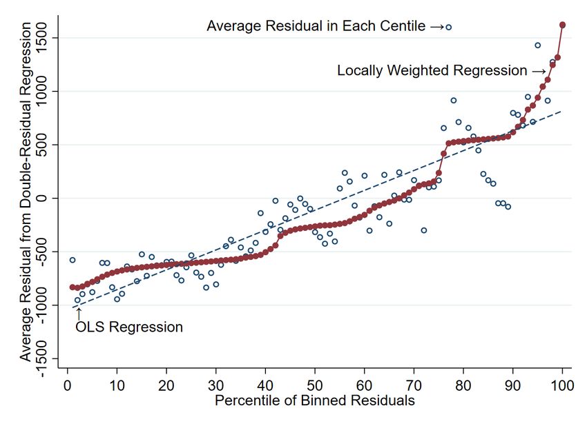
There is a growing interest in economics in evaluating the net cost of public policies when
causal eects on tax revenue and interactions with other policies are accounted for. The
dierence between a program's budgetary cost and net cost depends on behavioral responses
to the programe.g.,
scal externalities (Hendren, 2016)and whether other programs are
complements or substitutes. Understanding the net cost of public programs is important for
policymakersand the voting publicin deciding which programs to fund and to potentially
expand. This paper is one of the
rst comprehensive attempts to calculate a program's net
cost by estimating eects on several sources of tax revenue and public assistance spending.
The Earned Income Tax Credit (EITC) is one of the U.S.'s most important anti-poverty
programs, helping 28 million families at a budgetary cost of $73 billion in 2017. Previous
research shows that the EITC improves outcomes for lower-income mothers and their children
(discussed in section I), but the program's net cost to government and taxpayers is unknown.
Previous research shows that the EITC has led many lower-income mothers to join the
labor force (Eissa and Liebman, 1996; Meyer and Rosenbaum, 2001; Eissa et al., 2008;
Bastian, 2018). If true, this response likely impacts government revenue. Whether the
EITC's net cost is more or less than the $73-billion budgetary cost is theoretically ambiguous
and depends on whether these newly working mothers pay more taxes and whether the EITC
is a complement or a substitute for using other public-assistance programs. If the EITC
increases the employment of lower-income mothers, this would increase various sources of
tax revenue, decrease public-assistance spending, and lower the EITC's net cost. However,
if working mothers become eligible for public bene
ts that require a work history, such as
unemployment and disability insurance bene
ts, this would increase the EITC's cost.
We estimate the EITC's impact on labor supply, taxes paid, and public assistance received
with an identi
cation strategy that exploits variation in EITC eligibility, generated from
three decades of plausibly exogeneous EITC policy changes. One simple and transparent way
to capture these policy changes is to use one EITC parameter at a time. For example, the
maximum possible EITC bene
ts available to each household (M axEIT C ), varies by year,
1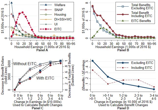
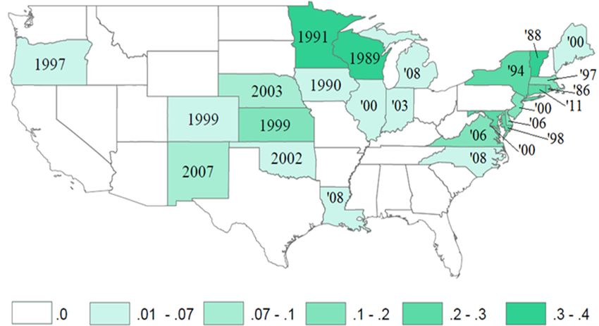
state, and number and age of children (see Figures 1 and 2), and is independent of income
and actual EITC eligibility. In addition to M axEIT C , we use other EITC parameters and a
simulated instrument (SI) approach that implicitly captures all EITC parameters and policy
changes. We use OLS, IV, and SI approaches to estimate shorter- and longer-run eects,
using dierence-in-dierences and event-study approaches.
We use newly available administrative data that links individuals in the 19892016 Cur-
rent Population Survey's Annual Social and Economic Supplement (CPS ASEC) to Internal
Revenue Service (IRS) Form 1040 returns. Because lower-income households often misreport
their income in survey data and income misreporting has steadily increased over time (Blank
and Schoeni, 2003; Meyer and Sullivan, 2003; Meyer et al., 2018), it is important to have
accurate administrative data to estimate the EITC's impact on earnings, tax credits, and
taxes paid. These linked data contain demographic details and public assistance usage not
available in tax data, as well as accurate income information, each of which is required to
estimate the EITC's net cost. Our sample includes 1.2 million women, ages 1964.
We
rst test whether the EITC increases employment and earnings, since there may be
little reason to expect eects on taxes and public assistance if labor supply is not aected. We
nd that each $1,000 increase in M axEIT C increases average annual earnings by $558 (in
2016 dollars), EITC bene
ts by $349, and employment by 0.6 percentage points, re
ecting
a participation elasticity of 0.33. Although previous studies have estimated the EITC's
employment eects (see section I), our data allow us to test the accuracy of studies relying
on survey data or a single EITC policy change. We also provide some of the
rst evidence
that EITC expansions after 2000 continued to increase labor supply.
Having found eects on labor supply, we turn to our main outcomes: taxes paid and
1
public assistance received. We
nd that a $1,000 increase in M axEIT C increases taxes
paid ($92) and reduces public assistance received (-$243). Eects are concentrated among
1 Labor supply changes may aect these outcomes since average and marginal tax rates for lower-income
families are often over 50 percent when public assistance is accounted for (Mok, 2012; Kosar and Mo
tt,
2017). We calculate eective tax rates on public bene
ts in Figures 3A and 3B (discussed in section II.B).
2
unmarried and lower-educated mothers and are robust to various sets of controls. For every
$349 in EITC spending, government revenue increases by $290, a 83 percent self-
nancing
rate. In other words, the EITC's net cost is only 17 percent of the budgetary cost. Our
results imply that the 2017 EITC provided $73 billion to low-income families at a net cost of
2
only $12 billion, costing the government less than the school lunch and breakfast programs.
In addition to tax revenue and savings on public spending, previous research shows that
the EITC improves health, decreases crime, and improves children's outcomes (see section
I). Accounting for the social value of these outcomesindependent of the private value
provides even stronger evidence that the EITC pays for itself (see section V.F).
Our results contribute to a literature on how policies can help pay for themselves, as
Brown et al. (2015)
nds for Medicaid, Denning et al. (2017)
nds for Pell Grants, Andresen
and Havnes (2018)
nds for childcare subsidies in Norway, and Michalopoulos et al. (2005)
and Michalopoulos (2005)
nd for a Canadian welfare reform experiment. These studies
nd
that these policies increased earnings and income tax revenue.
Our hypothesis is that M axEIT C is not associated with our outcomes of interest, except
through increased labor supply. For example, if EITC expansions occur during economic ex-
pansions and appear to increase taxes paid, estimates may re
ect not just EITC-led changes
in labor supply, but also a strong economy. We account for these types of potential con-
founders by testing for pre-trends and by controlling for state time trends and state × year
factors interacted with demographic traits and number of children.
Regarding potential EITC expansions today, our results show that (1) the EITC's net
cost depends on the target population's labor-supply elasticity and current level of public
assistance and (2) the EITC has largely paid for itself because low-income mothers are eligible
for other (substitute) programs. An EITC expansion for adults without children would likely
increase labor supply and taxes paid, but may have little impact on public assistance, since
adults without children receive little welfare, food stamps, and public housing. However,
2 This is not a perfect comparison since it compares the net cost of the EITC with a budgetary cost.
Eects on children's health, children's education, etc., would aect the school meals' net cost.
3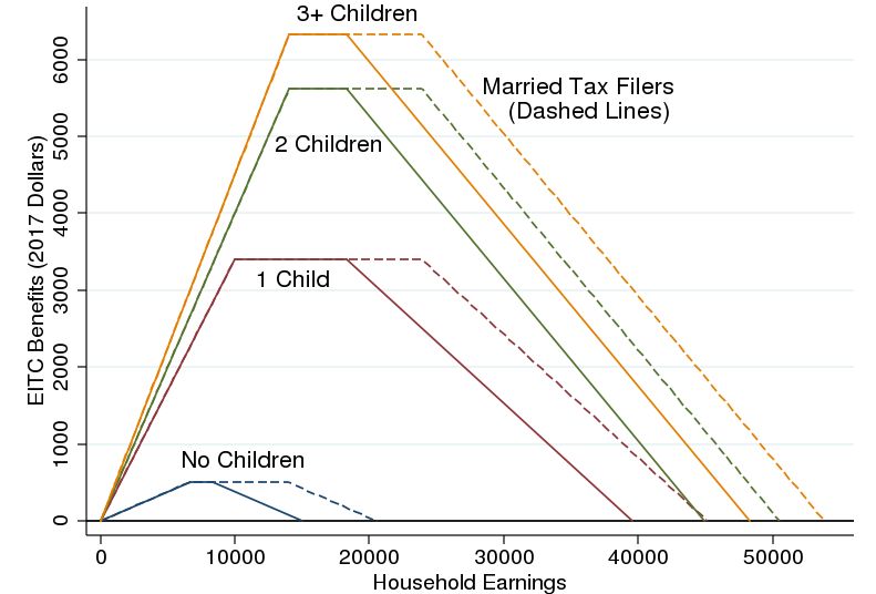
there has been a steady increase in DI and SSI (Autor and Duggan, 2006; Milligan and
3
Schirle, 2017), representing potential
scal savings (discussed in section VI).
Regarding social welfare, Hendren (2016) argues that a policy's impact on government
revenue is a su
cient statistic (Chetty, 2009a) for social-welfare analysis. Hendren (2016)
de
nes marginal value of public funds (MVPF) as the ratio of a policy's marginal bene
ts
to marginal costs. In section VII, we calculate the EITC's MVPF to be $3.18$4.23. Each
$1 of EITC spending generates over $3 in social value. For reference, the MVPF for the
top marginal income tax rate is $1.50$2 and a social-welfare-maximizing government could
increase the EITC
nanced by raising the top marginal income tax rateup to the point
where the MVPFs were identical for the EITC and for top marginal tax rates.
I. EITC Background and Literature Review
The EITC is one of the most important anti-poverty programs in the U.S., pulling millions
of people out of poverty and helping 28 million families, at a cost of $73 billion in 2017. The
EITC is a refundable tax credit that provides an annual earnings subsidy to lower-income
workers. EITC bene
ts are determined at the tax-
ling-unit level and are a function of
annual earnings, number and age of children, state of residence, and mar status. The EITC
contains a phase-in region, where bene
ts increase with earnings; a plateau region, where
bene
ts do not change with earnings; and a phase-out region, where bene
ts decrease with
adjusted gross income. Figure 1 shows how the 2017 EITC varies by family type.
The EITC began in 1975 as a 10 percent earnings subsidy, worth up to $1,700 (2016
4
dollars), that did not vary by state, marital status, or number of children. In 1986, the
phase-in rate rose to 14 percent. In 1990, higher bene
ts were made available to parents
with 2+ children; in 1993, a small credit was extended to adults without children; and
between 1993 and 1996, the phase-in rate rose to 34 and 40 percent for households with 1
3 Increased income may also improve health and decrease crime, drug-use, and mortality (see section VI).
4 See Bastian (2018) for more about the 1975 EITC and its impact on working mothers.
4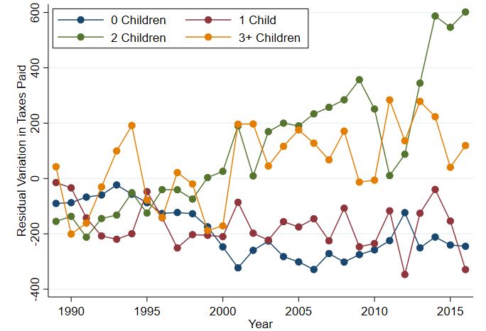
and 2+ children (a dierence worth up to $2,000). In 2002, the plateau region was extended
for married couples. In 2009, higher bene
ts were made available to parents with 3+ children.
Figures 2 and A.1 show the time-series for M axEIT C and the phase-in rate for house-
holds with 0, 1, 2, and 3+ children. Federal EITC bene
ts were worth up to $6,300 in 2017
(for households with 3+ children earning $14,000$24,000). Households with 0, 1, and 2
children were eligible for up to $500, $3,500, and $5,500 in federal EITC bene
ts.
Previous research shows that the EITC has numerous bene
ts for lower-income families.
Speci
cally, the EITC increases maternal employment (Homan and Seidman, 1990; Eissa
and Liebman, 1996; Meyer and Rosenbaum, 2001; Bastian, 2018), increases earnings (Dahl
et al., 2009), improves health (Evans and Garthwaite, 2014), decreases poverty (Hoynes and
Patel, 2015; Jones and Ziliak, 2019), decreases criminal recidivism (Agan and Makowsky,
2018), and helps children of EITC recipients by improving health (Hoynes et al., 2015; Averett
and Wang, 2015), test scores (Chetty et al., 2011; Dahl and Lochner, 2012), and longer-run
outcomes like educational attainment (Manoli and Turner, 2018; Bastian and Michelmore,
2018) and employment and earnings (Bastian and Michelmore, 2018). See Nichols and
Rothstein (2016) and Hoynes and Rothstein (2016) for EITC literature reviews.
Most EITC research focuses on the large 1990s expansions. In section V.A, we provide
some of the
rst evidence that the 2009 expansion continued to impact maternal labor supply.
Surprisingly, little is known about the EITC's impact on government budgets. If the
EITC increases employment and income, households may pay more payroll and state-income
taxes, and may receive less public assistance. Increased income for lower-income families
with high marginal propensity to consumemay pay more sales taxes. We account for these
factors and estimate the EITC's shorter- and longer-run net cost.
5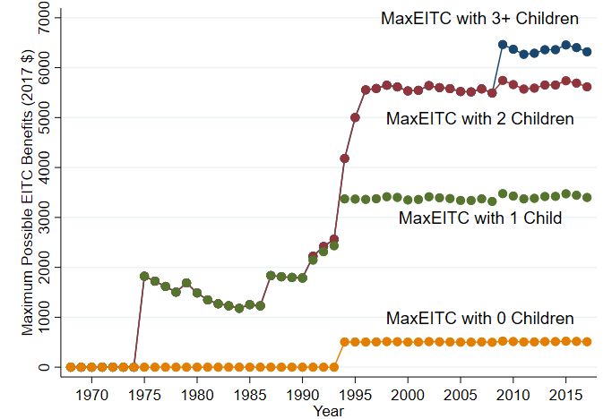
II. Conceptual Framework and Empirical Strategy
Our goal is to estimate the eect of EITC expansions on the government's net budget. For
a government budget (G) equal to tax revenue (T ) minus spending on public assistance
W elf are EIT C Other
(S ), the EITC (S ), and everything else (S ): G = T − S W elf are − S EIT C −
S Other . With no balanced budget restrictions, an EITC expansion costs ∂G/∂S EIT C . If
5
taxes and all other spending are unaected, then ∂G/∂S EIT C = −1. However, (1) fam-
ilies spending EITC bene
ts pay more sales taxes; (2) if the EITC increases labor supply
and earnings, households may pay more sales, payroll, and state-income taxes, and become
6
eligible for less in welfare bene
ts; and (3) previous research (see section I) shows that
the EITC improves health, decreases criminal recidivism, and improves children's long-run
outcomes, likely reducing spending on public health and incarceration, and increasing future
tax revenue and decreasing future public assistance spending. As a result, ∂T /∂S EIT C > 0,
∂S W elf are /∂S EIT C < 0, and ∂S Other /∂S EIT C < 0. The more that the EITC pays for itself,
the closer that ∂G/∂S EIT C gets to zero (and potentially even becomes positive).
We directly estimate ∂T /∂S EIT C in section IV.B and ∂S W elf are /∂S EIT C in section IV.C.
We then discuss other EITC research related to ∂S Other /∂S EIT C and calculate back-of-the-
envelope values for these components in section V.F. The lower the EITC's net cost, the lower
the amount of tax revenue required to fund an EITC, and the lower that a government's
redistribution preferences would have to be in order to have or expand an EITC.
II.A. De
ning the EITC Treatment Variables
We de
ne M axEIT C as the maximum possible federal EITC bene
ts that a family could
7
receive, given the year and number and age of children. M axEIT C captures three decades
of plausibly exogenous policy variation and is independent of income and actual EITC receipt,
5 That is, ∂T /∂S EIT C = ∂S W elf are /∂S EIT C = ∂S Other /∂S EIT C = 0
6 ∂S W elf are /∂S EIT C is a function of public assistance generosity and take-up rates, among other things.
7 The R-squared statistics from regressions of M axEIT C on number of children FE or year FE shows
that 73 and 13 percent of the variation in M axEIT C can be explained by number of children and year FE.
6
which are associated with socioeconomic status and our outcomes of interest. Previous
studies have used M axEIT C to estimate the EITC's eect on lower-income families (e.g.,
Hoynes et al. (2015), Hoynes and Patel (2015), Bastian and Michelmore (2018)). The mean
and standard deviation of M axEIT C are $2,260 and $2,156 (Table 1). Figures A.2 and A.3
show how the distribution of M axEIT C varies by number of children and varies over time.
Figures 2 and A.1 show the time-series for M axEIT C and the phase-in rate for house-
holds with 0, 1, 2, and 3+ children. Figure A.4 plots the residual variation from a regression
of M axEIT C on the full set of controls (see section III). Averaging residuals within each year
× number-of-children bin reveals trends that resemble the unadjusted M axEIT C trends in
Figure 2, suggesting that M axEIT C cannot be explained by trends in observed covariates.
The largest EITC policy changes occurred in the 1990s; many studies compare women
with 0, 1, or 2+ children, before and after this EITC expansion, to identify various outcomes.
Our empirical strategy of using M axEIT C implicitly nests this approach.
In deciding whether to use state EITCs, we test the exogeneity of state EITCs and
nd
some evidence that they are endogenous with other state policies and economic conditions
(Appendix B). Although we do not use state EITCs in the main analysis, we
nd similar
results when de
ning M axEIT C by federal, state, or federal + state (Table A.1) and we do
use state EITCs to estimate eects on aggregate state-level outcomes (section V.D).
If labor supply responses occur primarily on the extensive margin (as most evidence
shows (Meyer, 2002)), M axEIT C and the phase-in ratewill largely capture the EITC's
work incentives. However, these parameters may not capture intensive margin incentives or
some policy changes, such as extending the EITC plateau region for joint
lers. To capture
all EITC parameters and policy changes, we use a simulated-instrument approach.
7
II.B. Outcomes of Interest
Labor Supply: We test whether the EITC increases labor supply and earnings (as previous
8
studies have found) to motivate why the EITC may aect taxes and public assistance.
EITC Bene
ts: M axEIT C is associated with higher EITC bene
ts since (1) increased
employment may lead new workers to begin receiving the EITC and (2) those already working
and receiving the EITC may receive more bene
ts. Without the IRS EITC recipient
le,
we do not observe actual EITC bene
ts, but Jones and Ziliak (2019) shows that matched
IRS-CPS datawhich we useenables very accurate imputation of EITC bene
ts.
Taxes Paid: We look at payroll, sales, and unemployment insurance (UI) taxes. The
payroll tax rate is 15.3 percent, split between employers and workers, with the incidence
falling mostly on workers (Gruber, 1997; Deslauriers et al., 2018). We calculate payroll taxes
using a tax simulator. Payroll taxes are often paid back as Social Security bene
ts, and we
discuss their value in section V.E. We impute (1) sales taxes using state sales tax rates and
decomposing spending into taxable and non-taxable bins (Table E.3) and (2) federal and
state UI taxes from annual data. Details on these variables are in Appendix D.
Public Assistance Received: We look at welfare (i.e., AFDC or TANF), food stamps
9 10
(SNAP), public housing, disability (DI) and UI, Supplemental Security Income (SSI), and
workers' compensation (WC) bene
ts. Since public assistance is under-reported in survey
11
data, these estimates may be attenuated (Meyer and Mittag, 2015).
Figures 3A and 3B illustrate the relationship between public assistance bene
ts and
household earnings. Each Panel B shows that average bene
ts for mothers with no household
earnings is about $7,000 ($10,000 for unmarried mothers); average bene
ts fall by more than
8 For example, Homan and Seidman (1990), Dickert et al. (1995), Eissa and Liebman (1996), Meyer and
Rosenbaum (2001), Grogger (2003), Hotz and Scholz (2006), Eissa et al. (2008), and Bastian (2018).
9 Increased earnings while on public housing could decrease government spending when the number of
units is
xed, but not for housing vouchers where the budget is
xed. However, if households lose public
housing eligibility, bene
ts would go to a family on the waitlist and government spending would not change.
10 UI bene
ts require working at least one quarter in the previous year and being laid o by an employer.
11 Meyer and Mittag (2015)
nd that 40, 60, and 35 percent of SNAP, TANF/SSI, and subsidized housing
recipients report receiving zero bene
ts, and among households that report receiving public assistance, the
value of SNAP, TANF/SSI, and subsidized housing is underreported by 6, 40, and 74 percent.
8
$1,000 for every $5,000 in earnings, reaching about $1,500 for households earning $30,000
12
(corresponding to a full-time job at $15 per hour). Panel C shows the dierence in bene
t
levels between households with various levels of earnings to those with no earnings, with
and without the EITC. Finally, Panel D shows the implied eective tax rates on bene
ts,
with and without the EITC. Households earning up to $10,000, $10,000$20,000, and over
$20,000 face marginal bene
t tax rates of about 50, 25, and 10 percent (80, 30, and 10
13
percent for unmarried mothers). However, with the EITC, tax rates are 1520 percentage
points lower for earnings below $20,000 and 1015 percentage points higher for earnings of
14
$20,000$50,000, due to the EITC's phase-in and phase-out regions (Figure 1).
Although Figures 3A and 3B cannot be interpreted causally (i.e. for a given household's
change in earnings), they provide an idea of how much bene
ts may change for a mother
deciding whether or not to work. For example, not working versus working full time near
the minimum wage and earning $15,000 may result in about $5,000 less non-EITC public
assistance ($7,000 for an unmarried mother).
II.C. Estimating Equations
We use equation (1) to estimate average treatment eects on the outcomes discussed above.
Yist = α0 + α1 M axEIT Cg(i),t + α2 Xist + γs1 + γt2 + ist (1)
Equation (1) is a generalized dierence in dierences. M axEIT C is in $1,000 units (in CPI-
adjusted 2016 dollars). α1 measures the eect of an additional unit of M axEIT C on each
outcome Yist . State and year FE are denoted by γs1 and γt2 . Demographic traits, annual state-
level factors, state time trends, and numerous interactions are in Xist . ist is an idiosyncratic
12 Panel A in Figures 3A and 3B decompose public assistance into EITC, AFDC/TANF, SNAP, public
housing, and DI, SSI, Workers Compensation, and UI.
13 Previous research also shows that lower-income families face high average and marginal tax rates when
public assistance is accounted for (Mok, 2012; Kosar and Mo
tt, 2017).
14 Kaplow (2011) also points this out: the EITC is equivalent to making the phase-out of other transfers
more gradual.
9error term. Standard errors are robust to heteroskedasticity and clustered at the state level
to address serial correlation within a state over time (results are similar if clustered at the
level of treatment: year by number of children). We use CPS person weights.
We also test for heterogeneous eects with equations (2) and (3), since the EITC has
larger eects on unmarried and lower-educated mothers (Eissa and Hoynes, 2006).
Yist = β1 M axEIT C ×M arriedist +β2 M axEIT C ×U nmarriedist +β3 Xist +γs1 +γt2 +ist (2)
Yist = δ1 M axEIT C ×LowerEdist +δ2 M axEIT C ×HigherEdist +δ3 Xist +γs1 +γt2 +ist (3)
III. Linked CPS-IRS Data and Tax Simulator
We link the 1990, 1995, 1996, and 19982017 CPS ASEC to IRS Form 1040 income tax
returns, using an internal Census Bureau dataset containing a protected identi
cation key
15
(PIK). The CPS ASEC is administered in March and asks questions about the preceding
tax year. Upon linking datasets, we replace self-reported income, earnings, and marital
16
status with the 1040 values whenever possible, which reduces measurement error. We use
survey data for observations without a 1040. Since tax data report household-level income,
we capture individual earnings by assigning the full amount of household earnings to single
and head of household
lers, and by splitting the amount for married
lers in the same ratio
as their self-reported CPS ASEC earnings. Since this may introduce measurement error, we
also run household-level regressions where we do not split up earnings (Table A.9).
The sample consists of 1.2 million women 1964 years old who are not child dependents,
15 PIKs map to a unique Social Security Number (SSN). Tax data from 1991 to 1994 and 1997 are not
available for linking at Census. In 2006, the CPS ASEC stopped collecting SSNs, and probabilistic matching
(based on name, address, date of birth, etc.) is used to create PIKs (Layne et al., 2014). Data are compared
against a master address
le by name and date of birth, leading to PIK rates around 90 percent in most
years of data. All personally identifying information is removed for research purposes. Appendix F shows
PIK rates over time. Table F.2 shows the main estimates reweighted by the probability of not having a PIK.
16 Table E.1 crosswalks labor supply results using: CPS data; CPS data with administrative marital status;
CPS data with administrative earnings; and CPS data with administrative marital status and earnings.
10regardless of whether they or their spouse
led a 1040. We use a wide age range to estimate
the overall eect of the EITC on government budgets (although keeping older women in the
sample may attenuate some of the results, see footnote 18). We also run analysis using the
sample of all households (section V.D) to capture potential spillover eects on men.
Tax Simulator: The Bakija tax simulator (Bakija, 2014) calculates various state and
federal taxes paid and credits receivedincluding EITC bene
tsusing dozens of input
variables (e.g., income, number of children,
ling status). We identify tax-
ling units based
on family traits reported in the CPS ASEC (details in Appendix E). We would not need
a tax simulator if the 1040 data had the EITC refund (it does not) and if EITC take-up
was 100 percent. Although we do not observe actual EITC bene
ts, Jones and Ziliak (2019)
do, and they
nd that EITC payments calculated using the CPS-IRS data and Bakija's tax
simulator are very close to actual EITC payouts reported in the IRS EITC recipient
les
17
(and much more accurate than payments calculated from survey data alone).
Summary Statistics: Table 1 shows summary statistics and Table E.2 describes the
variables we use and whether they are derived from federal and state policy, the CPS ASEC,
IRS Form 1040, or the tax simulator. Women in the sample average 41 years old; have 0.8
children; 41 percent have a high school degree or less; 56 percent are married; 20 percent are
nonwhite; and 74 percent work and average 34 annual work weeks, 27 weekly work hours, and
$26,000 and $58,000 in individual and household annual earnings (in 2016 dollars). Women
receive $406 in EITC bene
ts; pay $3,716, $618, and $258 in payroll, sales, and UI taxes; and
receive $1,110 in public assistance, broken down into welfare ($98), public housing ($205),
SNAP ($306), DI ($96), SSI ($192), WC ($49), and UI ($168).
Control Variables: For each outcome, we show estimates are robust to various sets of
controls. In Table A.2, columns 17 progressively add controls for number of children
xed
eects (FE); year and state FE; education, race, marital status, age, and having a child
17 The Bakija calculator produces similar estimates of tax liability and EITC bene
ts as NBER's TAXSIM
(Jones and Ziliak, 2019). The choice of calculator was due to prohibitions on sending the CPS-IRS data
outside of Census to run TAXSIM on an external server. Complete details on Bakija's simulator are here:
https://web.williams.edu/Economics/wp/BakijaIncTaxCalcDoc.pdf.
11under 5; interacting marital status and education, with year, state, and number of children
FE; and state × year economic conditions and policies (from Appendix B) and state time
trends. Column 7 contains our preferred set of controls and is used throughout the analysis.
In columns 89, we show that results are robust to state × number of children FE and state
× year policies interacted with maternal demographic traits.
IV. Results
In this section, we estimate short-run eects of the EITC on various outcomes. In section
V.D we estimate longer-run eects.
IV.A. The EITC Increases Labor Supply and Income
Although previous research has found that the EITC increases maternal labor supply, our
data allow us to test the accuracy of studies that rely on survey data or a single EITC policy
change. As for parallel employment trends, previous work has shown parallel trends for
the 1990s EITC expansion (Meyer and Rosenbaum, 2001; Hoynes et al., 2015) and we show
parallel pretrends for the 2009 EITC expansion in Figures A.8A and A.8B. (We isolate the
eects of the 2009 EITC expansion in section V.A.)
Table 2 columns 1, 3, 5, and 7 show that a $1,000 increase in M axEIT C increases average
annual weeks worked (0.61), weekly work hours (0.50), employment (0.6 percentage points),
18 19
and annual earnings ($558). Estimates imply a participation elasticity of 0.33 (0.14).
Results are robust to alternate sets of controls (Table A.2); de
ning M axEIT C as federal,
state, or federal plus state (Table A.1); and using the EITC's phase-in rate (Table A.1). We
18 Results represent percent increases of 1.8, 1.8, 0.8, and 2.1. Estimates are smaller than EITC studies
that focus on younger women (Hoynes et al., 2015; Bastian and Michelmore, 2018), since age is negatively
associated with EITC response (Bastian, 2018, Table A.4). A log-log speci
cation yields estimates of 0.22,
0.21, and 1.28 for weeks worked, hours worked, and earnings plus EITC bene
ts (Table A.8).
19 Calculated as the change in log employment rates divided by the change in the log net-of-
tax-and-transfer income (following Chetty et al. (2012, Apx. B)). Using estimates and means in
Tables 2 and 3: [log(.736+.006)-log(.736)]/[log(25,170-4,544+1,111+444+ 349-243-110+558)-log(25,170-
4,544+1,111+444)]=0.328. Similarly, we calculate an earnings elasticity of 0.6.
1220
nd that the EITC is responsible for a third of the 1990s increase in maternal employment.
Table E.1 con
rms that relying solely on self-reported earnings yields estimates that are
attenuated by a third. Crosswalking the results from the public-use CPS data to the linked
21
CPS-IRS administrative data, Table E.1 shows the two estimates are $419 and $558.
Table 2 columns 2, 4, and 6 use equation (2) to test forand
ndlarge positive eects
among unmarried mothers, and null or small negative eects among married mothers, con-
sistent with previous research (Eissa and Hoynes, 2004; Yang, 2018). For married women,
a $1,000 increase in M axEIT C decreases annual work weeks (-0.32), weekly work hours
(-0.24), and employment (-1.4 percentage points). Because bene
ts are based on household
earnings, the EITC discourages work for some secondary earners. For unmarried women,
estimates are large and positive for weeks (2.75), hours (2.22), and employment (5.1 percent-
age points). Earnings estimates are also signi
cantly larger for unmarried women ($832 vs
22
$440). Among lower-educated unmarried women, we
nd even larger eects (Table A.3).
Although the EITC decreased labor supply among married mothers, the eect on unmarried
mothers is su
ciently large to result in a positive average eect.
Results are similar using a simulated instrument (SI) approach that implicitly captures all
EITC parameters and policy expansions, while also eliminating endogenous decisions about
household income and family structure (Currie and Gruber, 1996; Bulman and Hoxby, 2015;
Pilkauskas and Michelmore, 2018). We construct SIs by (1) using the 1989 CPS data (the
rst year in our sample) and calculating the EITC bene
ts that households would be eligible
23
for in each year between 1989 and 2016 using the actual annual EITC policy structure;
(2) collapsing average EITC bene
ts into (state × year × number of kids) bins, using CPS
ASEC weights and federal or federal plus state EITCs; and (3) merging these SIs into the
20 Calculated as: (estimate of 0.6) × (1990s change in average maternal M axEIT C : 4.5-1.7) / (1990s
change in maternal employment rate 0.77-0.72) = 0.33. Meyer and Rosenbaum (2001)
nds that the EITC
is responsible for about 60 percent of the 1990s increase in working mothers, though our estimate may be
smaller because our sample includes older women up to age 64.
21 Table E.1 shows that administrative IRS measures of marital status and earnings are both important.
22 Table A.3 shows (1) similar eects when the sample is restricted to unmarried women and (2) largest
eects among lower-educated unmarried mothers: 3.13 weeks, 2.52 hours, and 0.063 employment.
23 We keep household traits constant and CPI-adjust 1989 earnings and income into 19902016 values.
13main sample. In Table 5, we estimate equation (1), replacing M axEIT C with a SI, and
nd
that $1,000 in simulated EITC bene
ts increases weeks worked (1.40 to 1.46), work hours
(1.65 to 1.76), employment (1.7 to 1.9 percentage points), and earnings ($1,675 to $1,754).
Finally, Table 2 columns 910 show that $1,000 in M axEIT C increases average EITC
24
bene
ts by $349, with larger eects on unmarried than married women ($527 vs. $272).
These may be over-estimates since we do not observe actual EITC bene
ts (see section III)
and assume 100 percent take-up, while actual take-up is 7580 percent (Jones, 2014).
EITC bene
ts increase for two reasons: those already working and receiving the EITC
will receive more, and newly working women will start receiving the EITC. To disentangle
inframarginal and marginal bene
ts, we use the SI approach discussed above. Using equation
(1) and simulated EITC bene
ts as the outcome, we
nd that 72 percent of EITC bene
ts
are mechanical ($252 of $349), leaving 28 percent due to behavioral labor supply responses
($97 of $349). To assess whether the latter estimate is consistent with the earnings estimate
of $558, consider a few examples. Mothers with one and two children that began working
and earning $20,000 (or $25,000) would be eligible for about $3,200 and $5,400 (or $2,400
and $4,400) in EITC bene
ts. These EITC-to-earnings ratios are 16 and 27 percent (or 10
and 18 percent), consistent with the 17 percent ratio of our estimates ($97/$558).
At a cost of $349 per woman, the EITC increased female employment by 0.6 percentage
25
points and average annual earnings by $558. Next, we examine how the EITC's per-woman
cost of $349 changes when we account for changes in taxes paid and public assistance received.
24 M axEIT C 's impact on EITC bene
ts depends on where in the EITC schedule households are. For
those in the EITC's phase-in, plateau, phase-out, and beyond-phase-out regions (see Figure 1), a $1,000
increase in M axEIT C increases bene
ts by about $550, $950, $500, and $0 (with or without controls).
25 There were about 95 million U.S. women 1964 in 2016 and average M axEIT C was $2,200, implying
aggregate federal EITC bene
ts of $65 billion, close to the actual number of $73 billion. Any dierence
between these two numbers would be due to the dierence between EITC eligible households that do not take
up their bene
ts and EITC payments made in error; and EITC bene
ts received by single male households
not in our sample (Meyer (2010) estimates they receive about 8 percent of total EITC bene
ts).
14IV.B. Does the EITC Increase Various Sources of Tax Revenue?
Increased employment may increase payroll and UI taxes paid; higher income and EITC
bene
ts may increase consumption and sales taxes paid. Although many EITC recipients
pay no federal income tax, they pay payroll, sales, and UI tax rates of 15.3, 18, and 12
percent. (Section V.E discusses whether payroll and UI taxes should be considered revenue.)
We expect 2030 percent of an EITC recipient's earnings to be paid in taxes. From the
earnings and EITC estimates in Table 2 ($558 and $349), we expect $1,000 in M axEIT C
to increase taxes paid by around $100.
In Table 3 column 1, we use equation (1) and the sum of payroll, sales, and UI taxes
paid as the outcome. We
nd that each $1,000 increase in M axEIT C increases average
taxes paid by $92 (or 2 percent), suggesting that a contemporaneous increase in taxes paid
osets 26 percent of the EITC's per-woman cost ($349) to government. Results are robust
to alternate sets of controls (Table A.2). Decomposing the $92 shows payroll, sales, and
26
UI taxes of $70, $26, and $0.2 (Table A.5). We provide intuition for this tax estimate by
plotting the residualsaveraged into year × number-of-children binsfrom a regression of
taxes paid on the full set of controls (excluding M axEIT C ): Figure A.5 shows that the
trends in residuals follow the time-series trend in M axEIT C (Figure 2). In addition to
estimating the reduced-form eect of M axEIT C on taxes paid, we use (1) M axEIT C as
an IV for earnings and for EITC bene
ts and (2) a simulated instrument (SI) approach
(discussed in section IV.A). OLS estimates the population average treatment eect, while
an IV captures the local average treatment eect from compliers and will scale the OLS
estimates. Table 4 shows that the
rst stage is strongas would be expected from Table
2and shows that a $1,000 increase in earnings leads to $98 in taxes paid and a $1,000
26 Estimates do not exactly add up to $92 since they come from separate regressions. A log-log speci
cation
shows an EITC-taxes-paid elasticity of 0.86 (Table A.8). This may be an underestimate of the real value
since (1) local sales taxes are not accounted for; (2) most of these taxes are paid in the year prior to receiving
EITC bene
ts, and have a slightly higher present value. Our estimates imply that $14.6 billion in annual
payroll taxes can be attributed to the EITC (=95 million women × average M axEIT C of $2,200 in 2016
× $70) which constitutes about 1.8 percent of total payroll taxes in 2016 (payroll taxes totaled almost $800
billion and about 24 percent of total federal tax receipts).
15increase in EITC bene
ts leads to $267 in taxes paid (re
ecting the labor-supply response
associated with receiving the EITC). Using the EITC phase-in rate instead of M axEIT C
yields similar IV results (Table 4). For the SI, Table 5 shows that $1,000 in simulated EITC
bene
ts increases taxes paid by $372$392.
Since unmarried women have larger labor supply responses to the EITC, they should also
have larger increases in taxes paid. We test for this using equation (2) in Table 3 column
2 and
nd that a $1,000 increase in M axEIT C increases taxes paid by $157, compared
to a statistically smaller $70 among married women. Tax revenue osets 30 percent of the
per-unmarried-woman's cost of the EITC ($527).
IV.C. Does the EITC Decrease Public Assistance Usage?
We now test whether the EITC is a complement or a substitute for other public assistance
programs. In the context of the 1990s, Grogger (2003, 2004) show that the EITC reduced
welfare usage and Hoynes and Patel (2015) shows that the EITC reduced welfare and food
stamps usage. We expand on these studies by testing the EITC's eect on various types
of public assistance and whether the eects continued after the 1990s. Based on the $558
earnings estimate in Table 2, we expect $1,000 in M axEIT C to reduce public assistance
bene
ts by $140$280 since Figure 3A Panel C shows that for lower-income mothers, each
27
$1 of household earnings reduces bene
ts by $0.25$0.50.
Table 3 columns 36 use public assistance bene
ts as the outcome. A $1,000 increase
28
in M axEIT C decreases average bene
ts by $243, suggesting that a contemporaneous
decrease in public assistance spending osets 69 percent of the EITC's per-woman cost
27 Another way to set expectations is to use the facts that each $1 earned by a low-income parent reduces
TANF, SNAP, and public housing bene
ts by around $0.30 each (Nichols and Kassabian, 2012; Dean, 2017;
Center on Budget and Policy Priorities, 2017) and that take-up rates for these programs are 50, 60, and
1020 percent (Currie, 2004). $558 × [(.30 × .50) + (.30 × .60) + (.30 × .15)] = $209. However, working
mothers may also become eligible for bene
ts that require a work history (e.g. UI and DI).
28 Table A.6 shows the -$243 components: welfare (-$259), public housing (-$25), DI plus SSI (-$19), SNAP
($57), and UI ($1). The positive estimate on SNAP appears to con
ate the 2009 EITC expansion and the
2009 increase in SNAP bene
ts and recipients during the Great Recession (Ganong and Liebman, 2018)
since (1) the estimate changes to -$65 (s.e.=$10) when the sample is restricted to pre2009 and (2) Figures
4A and 4B show negative estimates (especially among unmarried mothers) before 2005.
16($349). We provide intuition for this estimate by plotting the residuals from a regression of
public assistance on the full set of controls (excluding M axEIT C ). These trends in Figure
A.6 follow the time-series trends in M axEIT C in Figure 2. We also
nd that $1,000 in
M axEIT C decreases the probability of receiving any bene
ts by 0.5 percentage point (or 3
29
percent). Results are robust to alternate controls (Table A.2); a log-log speci
cation yields
an estimated elasticity of -0.45 (Table A.8). Although our results are primarily driven by
reductions in cash welfare (Table A.6), we could not have known that ex ante. Furthermore,
eects on UI, DI, and SSI may become larger over time and merits further study.
In addition to estimating the reduced-form eect of M axEIT C on public assistance
received, we use (1) M axEIT C as an IV for earnings and for EITC bene
ts and (2) a
simulated instrument (SI) approach (discussed in section IV.A). Table 4 shows that a $1,000
increase in EITC-led earnings decreases public assistance by $189 and a $1,000 increase
in EITC bene
ts decreases public assistance by $516 (re
ecting the labor-supply response
associated with receiving the EITC). Using the EITC phase-in rate instead of M axEIT C
yields similar IV results (Table 4). For the SI, Table 5 shows that $1,000 in simulated EITC
bene
ts decreases public assistance received by $353.
Since unmarried women have larger labor supply and taxes-paid responses to the EITC,
they should also have larger decreases in public assistance usage. We test for this in Table
3 columns 4 and 6 and
nd that a $1,000 increase in M axEIT C decreases public assistance
received by unmarried women by $850 and decreases the probability of receiving any public
assistance by 3.1 percentage points (or 12 percent), compared to small positive eects among
30
married women ($20 and 0.6 percentage point). Less public assistance spending completely
29 Table A.7 shows that $1,000 in M axEIT C decreases the probability of receiving any welfare, public
housing, SNAP, and DI or SSI, by 2.8, 0.3, 0.2, and 0.1 percentage points, but increases UI by 0.1 percentage
points (we also
nd that $1,000 in M axEIT C decreases WIC bene
ts by $5; results not shown). Results
are consistent with Grogger (2003), who
nds that a $1,000 increase in M axEIT C reduce welfare use by
1.5 and 3.1 percentage points for among unmarried mothers whose youngest child is three and ten.
30 Components of the $850 are: welfare (-$767), public housing (-$92), SNAP ($5), DI + SSI + WC (-$11),
and UI ($11). Among married women, components of the $20 are -$39, $5, $79, -$22, and -$3. See Table
A.6. Table A.7 shows the change in the probability of receiving any of each type of public assistance.
1731
osets the EITC's per-unmarried-woman cost ($527). Although we do
nd an increase in
UI, we
nd much larger decreases in other bene
ts.
Based on the $832 earnings estimate in Table 2, we expected $1,000 in M axEIT C to
reduce public assistance bene
ts by close to $700 since Figure 3B Panel C shows that for
unmarried mothers, each $1 of earnings reduces bene
ts by up to $0.80. Although estimates
for unmarried women are a bit larger than we expected, our magnitudes are comparable to
Hoynes and Patel (2015), which
nds that $1,000 of M axEIT C reduces public assistance
32
by about $1,000 among unmarried mothers ages 2448 in the 1990s.
V. Alternate Explanations and Interpreting Results
V.A. Disentangling Welfare Reform and the 2009 EITC Expansion
The largest EITC expansions occurred in the 1990s, around the time of welfare reform.
Previous research disentangles these policy changes and shows that each policy had positive
eects on female labor supply (Meyer and Rosenbaum, 2001; Grogger, 2003, 2004), although
some recent work argues that the EITC receives too much credit (Mead, 2014, 2018; Kleven,
2019). If the EITC expanded while welfare was cutand we do not su
ciently control
for welfare reformour estimated eects of the EITC on public assistance may re
ect a
mechanical relationship, instead of increases in labor supply.
We disentangle these two policies by (1) showing that results are robust to
exibly con-
trolling for state × year × number-of-children measures of welfare reform interacted with
33
maternal education and marital status (Table A.2 column 8) and (2) providing some of
the
rst estimates of the eects of the 2009 EITC expansion, which raised M axEIT C from
31 This large response does not necessarily require a behavioral interpretation, since unmarried women
trade o these bene
ts with $1,359 in earnings and EITC bene
ts (Table 2).
32 One reason our estimates are a bit smaller is that our sample includes women up to age 64, less likely
to receive public assistance. Any potential attenuation in our public-assistance estimates will be similar for
Hoynes and Patel (2015), who also use CPS data.
33 These controls include maximum welfare with 14 children; when states introduced time limits; when
time limits began to bind; and whether states had a time limit.
18$5,400 to $6,300 for families with 3+ children (Figure 2).
Table 6 Panels A and B show that the EITC had positive eects on labor supply and
34
government revenue before and after 2005. Interacting M axEIT C with years before and
after 2005, eects are larger among unmarried women and, if anything, slightly larger after
2005. Figures 4A and 4B show the pre2005 and post2005 eect on each subcomponent of
taxes and public assistance: the strongest eects are increases in payroll and sales taxes and
decreases in welfare. Our results imply that the EITC is responsible for almost half of the
35
1990s decline in welfare.
Focusing on 20042014, we show parallel pretrends leading up to the 2009 EITC expansion
(Figures A.8A and A.8B) and use dierence in dierences to estimate the employment eect
on mothers with 3+ children. Table A.4 uses various sets of controls and compares mothers
with 3+ children to other groups of women, before and after 2009. Across speci
cations,
we
nd a 1.01.7 percentage point increase in employment (2.12.3 among lower-educated
mothers). That the 2009 EITC expansion had a positive eect on maternal employment is
consistent with previous research showing that the EITC increased maternal employment in
the 1970s (Bastian, 2018) and 1980s (Eissa and Liebman, 1996), in addition to the 1990s
(Meyer and Rosenbaum, 2001; Hoynes et al., 2015).
V.B. Diminishing Returns? Eects Over Time
If recent EITC expansions had diminishing returns, then our
nding that EITC expansions
largely pay for itself may have been true in previous decades, but not hold for recent
expansions or additional expansions today. We test for diminishing returns in three ways,
one of which uses OLS to estimate the EITC's eect before and after 2005 (see section V.A).
34 Each $1,000 of M axEIT C before and after 2005 increased average annual weeks worked (0.65 and 0.86),
weekly hours worked (0.49 and 0.70), employment (0.008 and 0.011), earnings ($310 and $812), taxes paid
($64 and $135), EITC bene
ts ($292 and $327), and decreased public assistance received (-$247 and -$241).
35 Calculated by: (estimate of $217 in Figure 4A) × (average M axEIT C increase of $1,500 among mothers)
× (95 million women ages 1964) × (49 percent of women have EITC-eligible children) = $15 billion out of
the $30 billion decrease in 1990s welfare spending.
1936
Second, we divide M axEIT C into categorical quartile bins and estimate equation (4).
X
Yist = θ0 + θ1c M axEIT C Quartilecist + θ2 Xist + γs1 + γt2 + ist (4)
c
Figures A.9, A.10, and A.11 illustrate that each EITC expansion has increased work weeks,
work hours, employment, earnings, EITC bene
ts, and government revenue. In general, we
cannot rule out constant or diminishing marginal eects over time.
Third, we use a locally weighted, double-residual regression (Cleveland, 1979). Figures
A.12 and A.13 show that the EITC's eect on taxes paid and public assistance received is
fairly linear and that recent expansions have continued to aect these outcomes.
These approaches all suggest that recent EITC expansions have continued to have positive
eects on labor supply and government revenue, perhaps suggesting that additional EITC
expansions today would continue to have positive eects.
V.C. EITC's Costs and Bene
ts for State, Federal Government
Results so far implicitly assume a unitary government, but tax revenue and public assistance
spending can be decomposed into state and federal components. Payroll taxes are paid to
the federal government, sales taxes to state governments, and UI taxes are paid to both
state and federal governments. For public assistance: welfare and UI bene
ts are paid by
state and federal governments, and the federal government bears the cost of public housing,
SNAP, SSI, DI, and WC (see Appendix D for program details).
Table 7 Panels A and B show how federal EITC expansions aect federal and state
government budgets. A $1,000 increase in M axEIT C leads to $349 in federal EITC spending
37
and $215 in federal revenue, a 61 percent self-
nancing rate. For states, a $1,000 increase
36 Bins means are 0, 506, 3351, and 5524. Results are similar using 5 or 6 bins. Equation (4) is identical
to equation (1) except M axEIT C is divided into four bins; the full set of controls is used, except children is
linear instead of FE (otherwise 0 and 3+ children is collinear with the lowest and highest M axEIT C bins).
37 $215 components are $70 in payroll tax revenue and -$158 -$25, $57, and -$19 in reduced welfare, public
housing, SNAP (SNAP results discussed in footnote 28), and DI/SSI/WC. $215 =$70+$158+$25-$57+$19.
20in M axEIT C leads to $21 in state EITC spending and $127 in state revenue, a net gain
of $106. Of course, not all states have an EITC: Panel C shows that states that ever had
an EITC net $122 (columns 13), compared to $73 for states without an EITC (columns
38
46). States with EITCs gain more from the federal EITC, perhaps because state EITCs
independently increase labor supply (shown in Table A.1 column 2) and raise awareness and
increase federal EITC take-up (Neumark and Williams, 2016). We provide some of the
rst
evidence that the EITC represents a transfer from federal to state governments.
V.D. Spillovers, the Longer-Run, and Aggregate Outcomes
The sign of the EITC's potential economic spillovers are theoretically ambiguous. On one
hand, the EITC may have negative spillovers on lower-skill workers if
rms respond to the
39
EITC by reducing pre-tax wages (Leigh, 2010; Rothstein, 2010). Most labor-demand-
elasticity estimates are 0.10.3 (Card, 1990; Borjas, 2003), meaning that our estimates may
40
be ignoring negative eects on the control group of EITC-ineligibles. On the other hand,
there could be positive labor-market spillovers if increased income and spending reverberate
41
through the economy (Carrington, 1996; Moretti, 2004; Black et al., 2005; Bartik, 2017).
We account for potential spillovers with household- and state-level analysis, using the
sample of all adult men and women. Although men are eligible for the EITC, previous
research
nds little impact on their labor supply (Eissa and Hoynes, 2004; Bastian, 2018),
implying that these estimates will average over positive responses by unmarried women,
38 $106 components are $26 in sales tax revenue and $101 in reduced welfare ($106 =-$21+$26+$101).
$122 components are $37 in state EITC spending, $31 in sales tax revenue, and $128 in welfare savings
($122=-$37+$31+$128). $73 comes from $17 in sales taxes and $56 in welfare.
39 Although Nichols and Rothstein (2016) shows that results in Leigh (2010) are likely biased upwards:
Leigh's estimates imply that employers capture approximately 500 percent of total EITC spending.
40 In the extreme case with perfectly elastic labor demand, all new workers are hired at the existing
wage and there are no negative spillovers. In the opposite extreme with perfectly inelastic labor demand,
EITC-eligible workers crowd out EITC-ineligible workers one for one, and the net eect of the EITC on tax
revenue may be near zero, although government spending could still decline if EITC-eligible workers (i.e.,
lower-income mothers) receive more public assistance than adults without children, which need not be true
if displaced workers begin receiving more public health services, DI and SSI, commit more crime, etc.
41 There is also a large macroeconomic literature on the
scal multiplier that focuses on public spending
(Auerbach and Gorodnichenko, 2012; Ilzetzki et al., 2013; Acconcia et al., 2014).
21small negative responses by married women, and null responses by men. Household-level
regressions are not able to detect spillovers on the control group of adults without children,
but are able to detect intra-household spillovers (i.e. these estimates should be smaller
than the eects on women if higher maternal labor supply is oset by lower spousal labor
42
supply). In contrast, aggregate state-level estimates re
ect the EITC's impact on mothers,
as well as anypositive or negativespillovers on men and women without children.
For households, Table A.9 shows that $1,000 in M axEIT C increases earnings ($1115),
taxes paid ($121), and EITC bene
ts ($550), and decreases public assistance ($221). Al-
though only the latter two estimates are statistically signi
cant, these results are consistent
with results in Tables 2 and 3 and provide little evidence for negative spillovers.
To estimate the EITC's longer-run eect on aggregate state employment, tax revenue, tax
lers, and welfare spending, we use equation (5) andalternate data sourcesstate reports
43
on these outcomes. To carry out this state-level panel analysis, we require state-level
44
variation, so we de
ne M axEIT C as the maximum possible state plus federal EITC.
Ysj = α0 + α1 M axEIT Cst + α2 Xst + γs1 + γt2 + st , for j ∈ [−7, 7] (5)
Figure 5 shows that a $1,000 increase in M axEIT C in year t has a contemporaneous eect
on employment, tax revenue, tax
lers, and welfare spending, and an increasingly large eect
over 34 years that remains through year t + 7.45 Bastian (2018), Eissa and Liebman (1996),
and Meyer and Rosenbaum (2001) also show that it took mothers a few years to fully respond
to the 1975, 1986, and 1993 EITCs. Estimates are robust to using logs and various sets of
42 These regressions are actually at the tax
ler-unit level; households may contain more than one tax
ler.
43 State employment data from BEA. State tax revenue data from Census. State welfare data from Health
& Human Services. Tax
lers from Tax Policy Center. Details and links to data in Figure 5 notes.
44 Unlike previous regressions, M axEIT C here only varies by state × year, not number of children. Year
FE ensure that we identify only o of state EITC changes. In Appendix B we
nd some evidence that state
EITCs may be endogenous with other state policies and economic conditions; although,
at pre-trends in
Figure 5 suggest that state EITCs are not a result of strong economic conditions.
45 A year after a $1,000 increase in M axEIT C , state employment, tax revenue, and welfare spending
change by 1.5, 5, and -9 percent. Eects on taxes and public assistance may also grow over time if these
women continue working, gain work experience, and see earnings growth (Dahl et al., 2009), which may
explain why tax revenue slowly increases after year t+3 and employment does not.
22You can also read