Oxygen export to the deep ocean following Labrador Sea Water formation
←
→
Page content transcription
If your browser does not render page correctly, please read the page content below
Research article
Biogeosciences, 19, 437–454, 2022
https://doi.org/10.5194/bg-19-437-2022
© Author(s) 2022. This work is distributed under
the Creative Commons Attribution 4.0 License.

Oxygen export to the deep ocean following
Labrador Sea Water formation
Jannes Koelling1 , Dariia Atamanchuk1 , Johannes Karstensen2 , Patricia Handmann2 , and Douglas W. R. Wallace1
1 Department  of Oceanography, Dalhousie University, Halifax, Nova Scotia, Canada
2 GEOMAR     Helmholtz Centre for Ocean Research Kiel, Kiel, Germany

Correspondence: Jannes Koelling (j.koelling@dal.ca)

Received: 21 July 2021 – Discussion started: 3 August 2021
Revised: 11 November 2021 – Accepted: 21 December 2021 – Published: 28 January 2022

Abstract. The Labrador Sea in the North Atlantic Ocean is         estimated (1.60 ± 0.42) × 1012 mol yr−1 of oxygen are added
one of the few regions globally where oxygen from the atmo-       to the outflowing boundary current, mostly during spring and
sphere can reach the deep ocean directly. This is the result of   summer, equivalent to 50 % of the wintertime uptake from
wintertime deep convection, which homogenizes the water           the atmosphere in the interior of the basin. The export of oxy-
column to a depth of up to 2000 m and brings deep water un-       gen from the subpolar gyre associated with this direct south-
dersaturated in oxygen into contact with the atmosphere. In       ward pathway of LSW is estimated to supply 42 %–71 % of
this study, we analyze how the intense oxygen uptake during       the oxygen consumed annually in the upper North Atlantic
Labrador Sea Water (LSW) formation affects the properties         Deep Water layer in the Atlantic Ocean between the Equator
of the outflowing deep western boundary current, which ulti-      and 50◦ N. Our results show that the formation of LSW is
mately feeds the upper part of the North Atlantic Deep Water      important for replenishing oxygen to the deep oceans, mean-
layer in much of the Atlantic Ocean.                              ing that possible changes in its formation rate and ventilation
   Seasonal cycles of oxygen concentration, temperature,          due to climate change could have wide-reaching impacts on
and salinity from a 2-year time series collected by sensors       marine life.
moored at 600 m nominal depth in the outflowing bound-
ary current at 53◦ N show a cooling, freshening, and increase
in oxygen content of the water flowing out of the basin be-
tween March and August. Analysis of Argo float data sug-          1   Introduction
gests that this is preceded by an increased input of LSW into
the boundary current about 1 month earlier. This input is the     Much of the global supply of oxygen to the deep ocean is
result of newly ventilated LSW entering from the interior,        concentrated in a few key regions where near-surface water
as well as LSW formed directly within the boundary cur-           sinks to great depth and spreads away from its source re-
rent. Together, these results imply that the southward export     gion (Talley, 2008; Gebbie and Huybers, 2011; Khatiwala
of newly formed LSW primarily occurs in the months fol-           et al., 2012). This process ventilates the deep ocean, sup-
lowing the onset of deep convection, from March to August,        plying oxygen to a vast volume of water that would oth-
and that this direct LSW export route controls the seasonal       erwise be barren and making it capable of sustaining life
oxygen increase in the outflow at 600 m depth. During the         (Rogers, 2015; Isozaki, 1997). One of the regions where
rest of the year, properties of the boundary current measured     such deep ocean ventilation occurs is the Labrador Sea, a
at 53◦ N resemble those of Irminger Water, which enters the       semi-enclosed marginal sea nestled between eastern Canada
basin with the boundary current from the Irminger Sea.            and western Greenland. Here, strong wintertime atmospheric
   The input of newly ventilated LSW increases the oxygen         cooling leads to buoyancy loss of surface waters that lay
concentration from 298 µmol L−1 in January to a maximum           above a weakly stratified water column, causing convective
of 306 µmol L−1 in April. As a result of this LSW input, an       overturning that homogenizes the upper 1000–2000 m of the
                                                                  ocean (Marshall and Schott, 1999; Yashayaev, 2007). Due

Published by Copernicus Publications on behalf of the European Geosciences Union.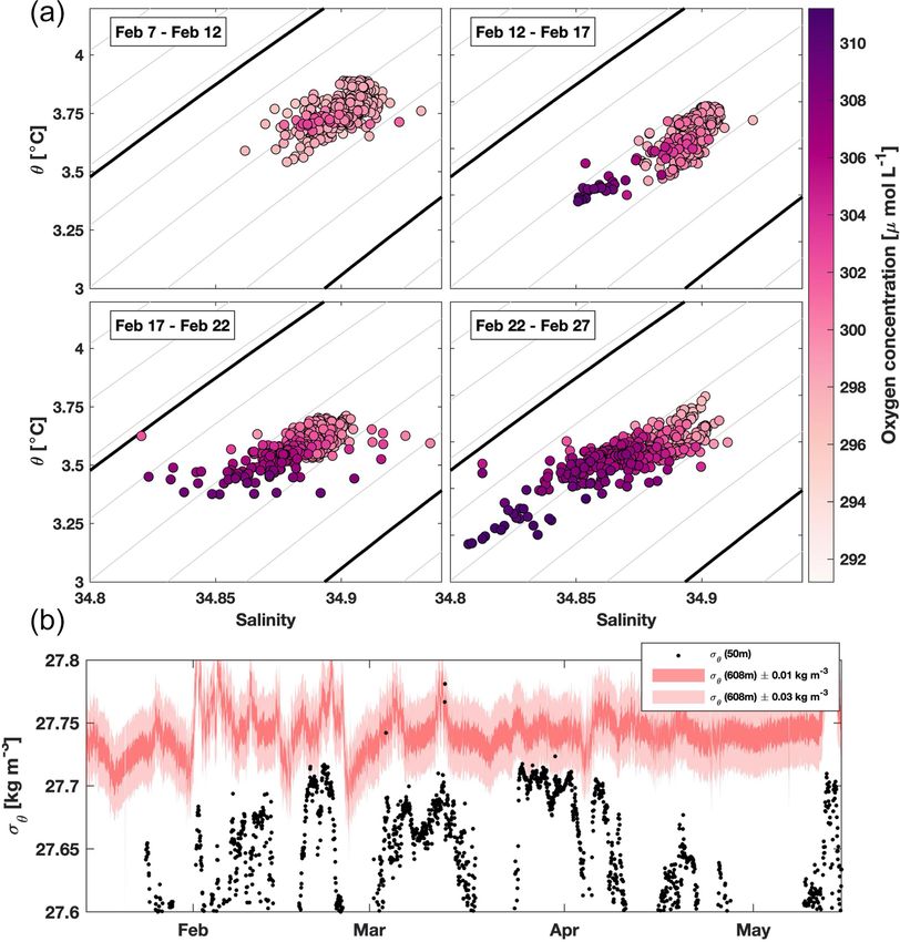
438                                                                              J. Koelling et al.: 53◦ N LSW oxygen export

to the great depths reached by convection in this region, it
is generally referred to as deep convection in order to dif-
ferentiate it from the much shallower-reaching convection
occurring in mixed layers throughout the global ocean, but
we will use the terms convection and deep convection in-
terchangeably hereinafter in the interest of brevity. During
the convection season, which typically lasts from January to
April, deep water masses that are low in oxygen are contin-
uously incorporated into the progressively deepening mixed
layer, which leads to a decrease in near-surface oxygen. This
results in severe air–sea gradients in oxygen concentration,
which, together with extreme atmospheric conditions, drive
intense uptake of oxygen during winter (Koelling et al., 2017;
Wolf et al., 2018; Atamanchuk et al., 2020).
   The climatological flow field in the Labrador Sea fea-
tures a cyclonic boundary current entering at the southern
tip of Greenland and exiting at the southwestern end of
the Labrador Sea, with only a weak mean flow in the inte-
rior (Fig. 1). At mid-depth, the boundary current entering        Figure 1. Mean salinity between 500 and 1000 m in the Labrador
the basin carries Irminger Water (IW), a water mass orig-         Sea, calculated from all available Argo float profiles between 2000
inating in the Atlantic ocean and modified in the subpolar        and 2020 (see Sect. 2.2 for details), averaged within overlapping
gyre, particularly the Irminger Sea (Cuny et al., 2002; Pacini    0.25◦ × 0.25◦ bins. Gray lines show the 1000, 2000, and 3000 m
et al., 2020). The cyclonic circulation in the Labrador Sea is    isobaths, vectors show mean currents at the depth of LSW from
linked to a doming of isopycnals in the center of the basin,      Fischer et al. (2018), and symbols correspond to positions of the
                                                                  SeaCycler mooring (red) and the 53◦ N array (magenta).
which supports deep convection in the interior (Marshall and
Schott, 1999). Different types of eddies, such as Irminger
rings and convective eddies, compensate the annual mean           ter (NADW) (Lazier, 1973), and it spreads throughout the
surface heat loss in the interior and help restratify the wa-     Atlantic Ocean, both as part of the Deep Western Boundary
ter column above the water mass formed during convection,         Current (Molinari et al., 1998; Toole et al., 2017) and in the
known as Labrador Sea Water (LSW) (Eden and Böning,               interior of the basin (Bower et al., 2009; Lozier, 2010). The
2002; Straneo, 2006; de Jong et al., 2014; Rieck et al., 2019).   signature of LSW is distinguishable in NADW properties far
Variability in atmospheric forcing, lateral fluxes of heat and    from the source region (Talley and McCartney, 1982; Rhein
freshwater, and the evolution of the mixed patch are main         et al., 2004; Le Bras et al., 2017), including elevated oxygen
drivers for interannual variability in the depth of convec-       concentrations compared to adjacent water masses (Atkin-
tion and in properties of LSW (Lazier, 1973; Yashayaev and        son et al., 2012). Although the importance of ventilation in
Loder, 2016). Much of the research has been focused on the        the Labrador Sea on NADW properties is readily apparent
deep convection region in the interior of the basin, but it has   from hydrographic data, the exact timing and mechanisms
been shown that convection can also occur within the bound-       of the southward export of LSW from the subpolar gyre are
ary current itself (Pickart et al., 1997; Palter et al., 2008).   not well established. Due to the weak mean currents in the
The densest water masses formed in the boundary current are       center of the basin (see Fig. 1), some studies have suggested
similar to the “classical” LSW formed in the interior, while      that much of the newly formed LSW remains in the inte-
convection over the continental slope forms a lighter water       rior for several years, with only a small fraction exported in
mass known as upper Labrador Sea Water or uLSW (Pickart           the months following convection (Rhein et al., 2002; Stra-
et al., 2002; Cuny et al., 2005). While the relative importance   neo et al., 2003; MacGilchrist et al., 2021). On the other
of boundary current convection is still uncertain, some model     hand, there is evidence of a rapid export pathway of newly
studies have suggested that it could account for a substantial    formed LSW which may be associated with convection ei-
fraction of the LSW that is eventually exported out of the        ther within or close to the boundary current (Pickart et al.,
region (Brandt et al., 2007; MacGilchrist et al., 2020).          1997; Brandt et al., 2007). An analysis from float data by
   The LSW formed each winter in the center of the basin          Palter et al. (2008) showed that both interior and boundary
is distinguishable in summertime hydrographic sections as a       convection can affect the properties of the outflowing bound-
cold, fresh water mass with high oxygen content, compared         ary current and suggested that eddies may play an important
to the warmer, saltier IW found in the boundary current near      role in the input of newly formed LSW into the boundary
Greenland (see Yashayaev and Loder, 2016, and Zou et al.,         current.
2020, for sections across the Labrador Sea). LSW is one of
the main water masses making up North Atlantic Deep Wa-

Biogeosciences, 19, 437–454, 2022                                                      https://doi.org/10.5194/bg-19-437-2022
J. Koelling et al.: 53◦ N LSW oxygen export                                                                                    439

   In this study, we use a novel dataset including moored oxy-
gen concentration measurements from the outflowing bound-
ary current at the southern exit of the Labrador Sea. The data
are recorded at the 53◦ N array (Zantopp et al., 2017), which
is part of the Overturning in the Subpolar North Atlantic
Program (OSNAP) (Lozier et al., 2017). We analyze annual
cycles of oxygen, temperature, and salinity, along with data
from Argo floats, in order to investigate seasonal variations
in the input of LSW into the boundary current and its export
out of the basin. Our results highlight how changes in proper-
ties of the outflowing boundary current over a seasonal cycle,
and resulting changes in the export of oxygen, are linked to
the formation and export of newly ventilated LSW.

2     Data and methods

2.1    Moored sensor data                                        Figure 2. Oxygen and salinity sections along the array from ship-
                                                                 board measurements collected during four mooring deployment and
Data used in this study were collected from May 2016             recovery cruises (see Sect. 2.2). Gray symbols show stations from
to May 2018 on the 53◦ N array in the boundary cur-              one representative cruise. Green symbols in (a) show deployment
rent at the exit of the Labrador Sea on moorings                 locations of the oxygen sensors, which were co-located with T –S
                                                                 sensors. Only data from the instruments at 600 m depth are used
K7 (52.86◦ N, 51.31◦ W), K8 (52.96◦ N, 51.31◦ W), K9
                                                                 in this study. The full coverage of current meters and T –S sensors
(53.14◦ N, 50.87◦ W), and K10 (53.39◦ N, 50.25◦ W) (west         is described in Zantopp et al. (2017). Black contours show the po-
to east in Fig. 1). Moorings have been deployed at the loca-     tential density range of 27.68 kg m−3 ≤ σθ ≤ 27.8 kg m−3 for LSW
tion since 1997 but in various configurations (Zantopp et al.,   and the σθ = 27.74 kg m−3 isopycnal which delineates the upper
2017). In the present setup, each mooring is equipped with       Labrador Sea Water (uLSW) above and classical Labrador Sea Wa-
Aquadopp and RCM current meters and SeaBird SBE 37               ter (cLSW) below.
instruments measuring conductivity, temperature (T ), and
pressure, which were also used to derive salinity (S). The
depths and positions of the instruments are optimized to mea-    (Pickart et al., 1997; Zantopp et al., 2017; Lozier et al., 2019)
sure the strength and properties of the boundary current ex-     or 27.7 kg m−3 (Zou et al., 2020), the former of which is
iting the Labrador Sea, including transports of different lay-   used as the definition of the LSW layer in this study. Within
ers (Zantopp et al., 2017). Since 2016, Aanderaa 4330 op-        the LSW layer, oxygen concentrations are elevated above
todes (Aanderaa Data Instruments, AS) have been deployed         1200 m, and the mean salinity is 34.86. The low-oxygen core
at select depths alongside T –S sensors to measure dissolved     below LSW centered at about 2000 m depth coincides with a
oxygen (O2 ) concentrations (Fig. 2a). We also use data from     salinity maximum, which is indicative of Northeast Atlantic
an Aanderaa 4330 oxygen optode mounted at 500 m depth            Deep Water (NEADW) (Yashayaev, 2007). Some authors
on the SeaCycler mooring in the central Labrador Sea (see        differentiate between “upper” and “classical” LSW (Pickart
Fig. 1 for location). For the SeaCycler optode, no co-located    et al., 1997), with the boundary between the two water
salinity data are available, and we estimate salinity used in    masses typically at a potential density of σθ = 27.74 kg m−3
Sect. 3.2 from a climatological T –S relationship at 500 m       (Kieke et al., 2006). The mean potential density at 600 m
calculated from Argo float data.                                 depth is 27.72 kg m−3 for K7 and 27.74 kg m−3 for K8–K10
   The deployment depths of the oxygen sensors on the 53◦ N      (Table 1), suggesting that sensors on these three moorings
array are shown in Fig. 2 along with mean oxygen and salin-      are near the interface between uLSW and cLSW (classical
ity sections along the array recorded with a conductivity–       Labrador Sea Water; see also Fig. 2).
temperature–depth (CTD) rosette. The majority of the O2             The mean salinity of the boundary current in the LSW
sensors were deployed at nominal depths of approximately         depth range decreases as it flows cyclonically around the
600 m or 1900 m, chosen to represent the LSW core, and a         basin (Fig. 1). At the 53◦ N array, the salinity is closer to
depth near the bottom of the LSW layer. Only the sensors         values found in the interior Labrador Sea compared to the
at 600 m depth are used in this study, and the deployment        Greenland side, consistent with the view that there is signifi-
and calibration information for these sensors is summarized      cant input of LSW from the interior. However, the water here
in Table 1. LSW is commonly defined in density space by          is still warmer and saltier than that found in the convective in-
a range of potential density σθ , with a lower boundary of       terior, suggesting that it is a mixture of LSW and IW, which
27.8 kg m−3 and an upper boundary of either 27.68 kg m−3         enters the Labrador Sea on the northern side at a mean core

https://doi.org/10.5194/bg-19-437-2022                                                      Biogeosciences, 19, 437–454, 2022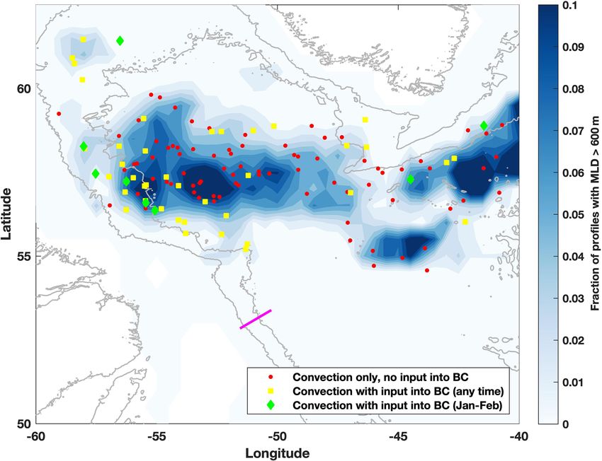
440                                                                                J. Koelling et al.: 53◦ N LSW oxygen export

Table 1. Deployment locations, depths, and drifts of the oxygen
optodes during 2016–2018.

  Mooring        Nominal          Mean     Optode          Drift
              deployment       potential    Serial   [µmol L−1 ]
                depth [m]       density    number
                              [kg m−3 ]
  K7                 608         27.72     052634          −5.8
  K8                 608         27.74     052631          −5.2
  K9                 610         27.74     052628          −2.5
  K10                610         27.74     052626          −6.1

depth of about 500 m and can be seen as a local salinity max-
imum near this depth (Pacini et al., 2020). In this study, we
will focus on the variability in properties in this LSW layer
using data from the sensors mounted at about 600 m on the           Figure 3. Example of Argo data used to track LSW input into the
moorings, representing the full width of the boundary current       boundary current after convection from float ID 6902589. (a) Tra-
from the shelf break area (K7, K8), via the core (K9), into the     jectory showing latest deep mixed layer measurement (blue star)
outer edge and recirculation regime (K10).                          and location of entry into boundary current (red star). Thick green
                                                                    line highlights the part of the trajectory from LSW formation to
2.1.1    Sensor calibration                                         crossing the 3000 m isobath. (b) Time series of mixed layer depth
                                                                    and maximum layer thickness, with green shading highlighting the
Temperature and salinity sensors were calibrated following          time from convection in the interior to entering the boundary cur-
the procedure outlined in Karstensen (2005). Briefly, the           rent. (c) Consecutive profiles of layer thickness in density space,
method involves attaching the sensors to a CTD rosette prior        going from convection (dark blue) to input into boundary current
                                                                    (light green).
to and after each deployment and comparing the data from
the different instruments at certain stop depths with the CTD
recording, which is calibrated with discrete bottle samples
                                                                       We also use data from the Argo program (Roemmich et al.,
taken throughout the cruise.
                                                                    2009), which are freely available online, including both in-
   Oxygen optodes were supplied with individual multipoint
                                                                    dividual float data and data products. The data from indi-
factory calibration, with an absolute accuracy of 1.5 % or
                                                                    vidual floats were downloaded from coriolis.eu.org, using
2 µmol L−1 (Tengberg et al., 2006; Tengberg and Hovdenes,
                                                                    all profiles flagged as “good” on the data selection service
2014), and powered by single-channel loggers (RBR Ltd.).
                                                                    that were found in the area of 50–65◦ N , 65–40◦ W be-
The optodes were further calibrated against Winkler samples
                                                                    tween 1 January 2000 and 8 September 2020 (Argo, 2020,
collected during CTD casts at the mooring locations during
                                                                    https://doi.org/10.17882/42182#77634), resulting in a total
deployment and recovery cruises in 2016 and 2018 to correct
                                                                    of 41 165 temperature and salinity profiles from 568 floats.
for sensor drift. The drift of the sensors during deployment
                                                                    These data were used to produce the mean salinity map in
ranged from −2.5 to −6.2 µmol L−1 or 0.4 % yr−1 –1 % yr−1
                                                                    Fig. 1 and are used to track the formation and boundary cur-
(see Table 1).
                                                                    rent input of LSW as described in Sect. 2.3. Data from the
                                                                    Argo mixed layer depth database by Holte et al. (2017) are
2.2     Additional datasets
                                                                    used in Fig. 7 in order to highlight the mean convection area.
In addition to the mooring data that are the focus of this study,      Bottom topography shown in Figs. 1, 3a, and 7 comes
we use ancillary data from a number of different sources,           from the SRTM15+ product (Tozer et al., 2019), which is
which will be briefly described in this section                     the most recent product based on Smith and Sandwell (1997).
   CTD data used in Fig. 2 were collected during four moor-         These data are also used to differentiate between the interior
ing deployment cruises in 2014 (cruise Thalassa MSM40),             and boundary current regions for the analysis of Argo data.
2016 (MSM54), 2018 (MSM74), and 2020 (MSM94). The                   Current vectors used in Fig. 1 are taken from the dataset de-
station spacing near the moorings was typically around              scribed in Fischer et al. (2018).
10 km, and the stations occupied during the 2016 cruise are
indicated in the figure. The sections shown in the figure were
produced by interpolating all measurements from the four
cruises onto a regular grid with 2.5 km horizontal and 1 dbar
vertical spacing using a Gaussian interpolation.

Biogeosciences, 19, 437–454, 2022                                                        https://doi.org/10.5194/bg-19-437-2022
J. Koelling et al.: 53◦ N LSW oxygen export                                                                                        441

2.3   Tracking Labrador Sea Water formation and input                     The evolution of layer thickness and mixed layer depth
      into the boundary current                                        shown in Fig. 3 is representative of a typical float measuring
                                                                       LSW formation in the interior that later enters the boundary
                                                                       current. Generally, after the initial profile measuring a deep
To evaluate the input of LSW into the outflowing boundary              mixed layer, surface restratification and mixing lead to a de-
current, we use data from Argo floats to investigate convec-           crease in maximum layer thickness, but the signature of LSW
tion regions and LSW input in Sect. 3.1 and 3.2. The pro-              remains detectable. To ensure that only floats moving with
file data are used to calculate mixed layer depths based on a          newly formed LSW were used, we discarded data from floats
density difference of 1σθ = 0.01 kg m−3 from the shallowest            with changes in maximum layer thickness of more than 50 %
measurement, which has been shown to be a suitable thresh-             between consecutive profiles. As a result, data from about
old in the subpolar North Atlantic (Piron et al., 2016; Zunino         12 % of all floats measuring convection were omitted from
et al., 2020). After the last convective profile for each sea-         the analysis, but the findings discussed in Sect. 3.1 do not
son, defined here as a mixed layer depth exceeding 600 m,              change qualitatively if all float data are used instead. The
we track the trajectory until the float enters the boundary cur-       layer thickness criterion is used only for floats measuring
rent. We define LSW input as a float crossing the 3000 m iso-          convection in the interior. For convection within the bound-
bath and subsequently staying in the boundary current for at           ary current, LSW input occurs at the time of the initial pro-
least two out of the next three profiles thereafter, similar to        file, and we only use the constraint that two of the next three
definitions used in previous studies (Georgiou et al., 2020).          profiles have to be in the boundary current.
A stricter criterion was also tested, requiring floats to subse-          In order to investigate the seasonal timing of LSW input
quently be exported south of 53◦ N within the boundary cur-            into the boundary current, we define a LSW input rate which
rent, reducing the number of floats used for the analysis by           is simply given by the number of floats measuring LSW input
about half. However, results are not sensitive to this choice,         at a given time divided by the total number of floats entering
with the curve shown in Fig. 9b being almost identical if this         the boundary current:
export criterion is used instead.
    During a typical Argo cycle, floats park at a depth of ei-                          n(t)
                                                                       InputLSW (t) =        ,                                      (1)
ther 1000 m or 1500 m for 10 d before descending to 2000 m,                              N
measuring a profile to the surface and staying there to trans-         where t is the time given as day of year in 5 d bins, n(t) is
mit the data, which typically last about 1 h but can be as much        the number of floats inputted during each time step, and N is
as 12 h for older float models (Lebedev et al., 2007). As a            the total number of floats measuring LSW input. This is used
result, the floats are not strictly following a water parcel, as       in Sect. 3.2 to compare the LSW input to the seasonal cycle
vertically sheared currents can carry them away from the wa-           of oxygen at K9. One possible caveat of this method is that
ter mass they had been advected with at depth. To ensure               it does not take into account the volume of LSW associated
that floats used for the calculation are following LSW, we             with each instance of input, which would require some in-
use layer thickness measurements to track them. Layer thick-           formation about the horizontal extent of each patch of LSW
ness is inversely proportional to the vertical density gradient,       measured by the floats. Furthermore, variations in the num-
and newly formed LSW is readily detected as a maximum                  ber of floats present in the region at different times could lead
(Yashayaev and Loder, 2016). An example of layer thick-                to biases in the resulting estimate of the LSW input rate.
ness measurements from a float measuring convection in the
interior of the basin and subsequently entering the bound-
ary current on the southwestern side is shown in Fig. 3. Ini-          3   Results
tially, the time series show mixed layer depth and maximum
layer thickness varying in concert, as the thickest layer is the       Time series of oxygen at 600 m nominal depth (Fig. 4)
actively convecting mixed layer (Fig. 3b). This is also ev-            show an overall similar picture at all sites: Starting in
ident in the last profile measuring convection, as the max-            February–March, high-frequency oxygen variability inten-
imum layer thickness is found at the lowest density mea-               sifies, and mean oxygen concentrations increase by around
sured, suggesting that no lighter water mass is present above          10 µmol L−1 , remaining elevated during spring. Subse-
the maximum associated with LSW (Fig. 3c, dark blue line).             quently, the short-term variability subsides, and beginning in
Subsequently, the mixed layer depth decreases to almost zero           July, oxygen concentrations decrease slowly throughout the
(Fig. 3b), indicating surface restratification, but a maximum          year until the next increase the following winter. The shift
in layer thickness remains. In the profiles (Fig. 3c), this can        in oxygen concentrations appears to occur in concert with
be seen as lower-density water accumulating above the maxi-            changes in temperature and salinity (Fig. 5). T –S changes
mum around σθ = 27.74 kg m−3 . The magnitude of the max-               occur largely along isopycnals, meaning that the effect of T
imum decreases through mixing with surrounding water, but              and S variations on density compensate each other. Correla-
it is still detectable in the profile as the float enters the bound-   tion between T and O2 is high for all of the sites, between
ary current.                                                           −0.80 and −0.94. Although some of this can be explained

https://doi.org/10.5194/bg-19-437-2022                                                           Biogeosciences, 19, 437–454, 2022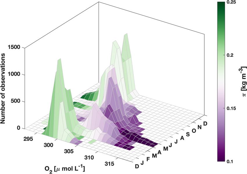
442                                                                                     J. Koelling et al.: 53◦ N LSW oxygen export

                                                                         3.1   High-frequency oxygen variability in
                                                                               February–April

                                                                         As oxygen concentrations at the mooring sites begin to in-
                                                                         crease in late February, there is a concurrent increase in the
                                                                         spread of the measurements (Fig. 4). In 2017, during the
                                                                         months of February, March, and April, oxygen concentra-
                                                                         tions at K9 vary between values typical of the months prior,
                                                                         between 297 and 301 µmol L−1 , and higher values ranging
                                                                         from 305 to 315 µmol L−1 , which subsequently persist until
                                                                         late June. During these months, the spread between the min-
                                                                         imum and maximum values measured in a single day can be
                                                                         as much as 15 µmol L−1 , and the standard deviation increases
                                                                         from 1.1 µmol L−1 for the 3-month period from 1 Novem-
                                                                         ber 2016 to 31 January 2017 to 4.2 µmol L−1 for 1 February
                                                                         to 30 April 2017.
Figure 4. Time series of oxygen concentration at 610 m for K7, K8,          This wide spread in the measured oxygen concentrations
K9, and K10 (a–d). Gray lines show original 15 min data, and black       is also reflected in differing temperature and salinity proper-
lines show time series filtered with a 10 d running mean. Note that      ties for a 20 d period in February (Fig. 6a). As for the overall
axis limits are 5 µmol L−1 lower in (a), but the range is the same for   dataset, the highest oxygen values occur at the lowest tem-
all panels.
                                                                         peratures and salinities. Starting from a cluster of points with
                                                                         higher temperatures and salinities for 7 to 12 February, wa-
                                                                         ter with properties of LSW begins to emerge in the following
by solubility changes, which are dependent on temperature
                                                                         days, and by 27 February, some of the measured T –S val-
(Garcia and Gordon, 1992), correlations between saturation
                                                                         ues are similar to those found in the center of the basin dur-
percentage and temperature are still high, between −0.58 and
                                                                         ing convection (see also Fig. 5). During this time, much of
−0.84. If changes in oxygen were simply due to temperature-
                                                                         the annual range of temperature, salinity, and oxygen prop-
driven solubility differences at a constant saturation percent-
                                                                         erties found in the 2-year record is observed within just 20 d
age, the correlation of saturation and temperature would be
                                                                         (see Figs. 5, 6a). High-frequency variability in properties at
zero. The fact that both saturation percentage and concentra-
                                                                         the beginning of the convection season was also observed
tion are correlated with temperature suggest that the changes
                                                                         in temperature measurements further upstream in the bound-
are associated with the presence of different water masses.
                                                                         ary current by Cuny et al. (2005). They concluded that LSW
In fall and early winter, measurements show warmer, saltier,
                                                                         was being formed within the boundary current itself and at-
and lower-oxygen water with a lower saturation percent-
                                                                         tributed the high-frequency variability to spatially varying at-
age, while colder, fresher water with higher O2 concentration
                                                                         mospheric forcing producing LSW with differing properties.
and saturation is predominantly observed in late winter and
                                                                         However, the fact that there is also a large spread in oxygen in
spring.
                                                                         Fig. 6a suggests that some of the water observed during this
   The majority of the T –S measurements lie roughly along
                                                                         time has not yet been ventilated. Instead, the variability could
a mixing line between typical endmembers for LSW and IW
                                                                         be a sign that the earliest convective activity is episodic and
(see Fig. 5 for reference). The clustering of measurements
                                                                         patchy, resulting in newly ventilated LSW being transported
between these two endmembers suggests that variability in
                                                                         with the boundary current alongside the lower-oxygen IW
properties at 53◦ N, including oxygen, is chiefly controlled
                                                                         found prior to the onset of convection.
by changes in the fraction of each source water mass found
                                                                            Although Cuny et al. (2005) showed that LSW forma-
in the boundary current.
                                                                         tion can occur in the boundary current, there is no evidence
   In the following sections, we will analyze the main fea-
                                                                         of local convection near 53◦ N in our data. While no near-
tures of the time series in more detail, discussing first the ini-
                                                                         surface instrument was deployed on the K9 mooring, data
tial oxygen increase in February and March and associated
                                                                         from about 50 m depth at K8 suggest that the boundary
higher-frequency variability using data from the K9 mooring
                                                                         current at 53◦ N remains stably stratified (Fig. 6b). Vertical
(Sect. 3.1). This is followed by an analysis of a complete sea-
                                                                         density gradients generally exceed the 1σθ = 0.01 kg m−3
sonal cycle of oxygen concentration at K9, covering convec-
                                                                         threshold often used to determine mixed layer depth in the
tion and the following restratification period in 2016–2017
                                                                         region (Piron et al., 2016), as well as the less stringent thresh-
(Sect. 3.2), and a brief analysis of the differences between
                                                                         old of 1σθ = 0.03 kg m−3 used by de Boyer Montégut et al.
the moorings (Sect. 3.3).
                                                                         (2004). This suggests that there is no active convection near
                                                                         the mooring sites during the study period. Instead, we con-
                                                                         clude that the water must be advected to the 53◦ N array from

Biogeosciences, 19, 437–454, 2022                                                             https://doi.org/10.5194/bg-19-437-2022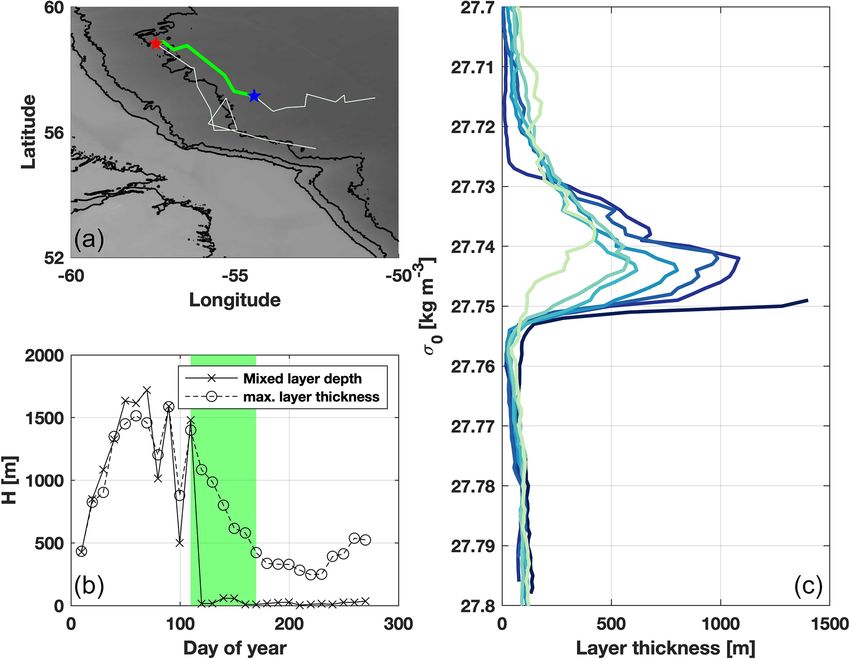
J. Koelling et al.: 53◦ N LSW oxygen export                                                                                           443

                                                                             Also shown in the figure are convection locations for all
                                                                          floats from the 2000–2020 period from the Argo data de-
                                                                          scribed in Sect. 2.2, using the last profile measuring a mixed
                                                                          layer deeper than 600 m. The points generally line up with
                                                                          the mean picture from the Holte et al. (2017) data, with dif-
                                                                          ferences between the two likely occurring due to continued
                                                                          modification during convection. Overall, the majority of the
                                                                          profiles measuring convection in both datasets are in the in-
                                                                          terior. Most of those floats that measure deep mixed layers
                                                                          inshore of the 3000 m isobath are located immediately adja-
                                                                          cent to the interior patch.
                                                                             A quantitative analysis of the relative importance of the
                                                                          different formation regions is beyond the scope of this study
                                                                          as the Lagrangian nature of Argo floats results in undersam-
                                                                          pling of fast-flowing boundary currents relative to regions
                                                                          with weak currents like the interior Labrador Sea. Nonethe-
Figure 5. Temperature and salinity diagrams at about 600 m nom-           less, our dataset reveals some features about the differences
inal depth from all four boundary current moorings, showing daily         between convection in the interior and within the boundary
averages. Colors correspond to oxygen anomalies relative to the
                                                                          current. The profile locations in Fig. 7 are color coded by
mean at each instrument, ranging from −10 µmol L−1 (blue) to
                                                                          whether or not the float enters the boundary current during
+10 µmol L−1 (red). Purple stars and shading show values from
the wintertime mixed layer at the SeaCycler mooring in the inte-          the same year using the definition of LSW input described
rior Labrador Sea (Atamanchuk et al., 2020), and green symbols            in Sect. 2.3. About half of the floats measuring convection
and shading show typical wintertime conditions of IW near Green-          in the interior remain there until the following convective
land, taken from Pacini et al. (2020). Potential density (σθ ) contours   season, consistent with model studies showing that newly
are drawn with a spacing of 0.025 kg m−3 , and solid black contours       formed LSW can remain in the interior for several seasons
show densities of σθ = 27.68 and σθ = 27.8 kg m−3 .                       (Straneo et al., 2003; Georgiou et al., 2020). Conversely,
                                                                          most of the floats measuring deep mixed layers inshore of
                                                                          the 3000 m isobath stay within the boundary current after-
upstream. The observations are consistent with LSW being                  wards, suggesting that a larger fraction of LSW formed in
formed in the interior of the basin and entering the bound-               the boundary current is exported out of the basin compared to
ary current along isopycnals (Georgiou et al., 2020). Alter-              LSW formed in the interior. Moreover, out of the more than
natively, the observed changes could also be explained by                 100 floats measuring convection to depths exceeding 600 m,
convective activity taking place within the boundary current              only six are subsequently found inshore of the 3000 m iso-
further upstream.                                                         bath in the months of January and February. The convection
   In order to identify the source of the LSW arriving at                 location of these floats is highlighted in Fig. 7 by green dia-
53◦ N in February, we use data from Argo floats to inves-                 monds. The floats found in the boundary current during this
tigate the timing of convection and input into the boundary               time measured either convection very close to the 3000 m
current. Figure 7 shows the fraction of profiles within 50 km             isobath, which allows them to enter the boundary current
of each 0.5◦ × 0.5◦ bin that measured mixed layers deeper                 quickly, or convection within the boundary current region it-
than 600 m based on the Holte et al. (2017) Argo mixed layer              self. This suggests that the initial arrival of the elevated oxy-
depth database. The most salient feature is a large area of               gen signal at the moorings in February is likely to be a result
deep mixed layers in the interior of the basin, near the mixed            of convection within, or close to, the boundary current.
patch often defined as the LSW formation region (Lazier,
1973; Yashayaev, 2007; Atamanchuk et al., 2020). The area                 3.2   Seasonal cycle
extends eastward and indicates a major interior ocean spread-
ing pathway that connects the Labrador Sea and Irminger Sea               To investigate the broader-scale variability, we look at the
(Talley and McCartney, 1982; Sy et al., 1997; Fischer et al.,             relation between oxygen and temperature and salinity for
2018; Zunino et al., 2020). Another region of increased oc-               the period of December 2016 to December 2017, covering
currence of deep mixed layers is found inshore of the 3000 m              a full annual cycle including convection and restratification.
isobath near 55◦ W, close to where Pickart et al. (2002) first            Figure 8 shows the evolution of the oxygen concentration
reported evidence of convection in the boundary current. No               throughout the year in the form of monthly histograms with
mixed layers deeper than 600 m are found in the boundary                  a bin size of 1 µmol L−1 . The color for each bin shows the
current south of 55◦ N, consistent with our findings from the             mean spiciness (π ), which is a tracer of T and S variations
mooring data that convection did not occur locally at 53◦ N.              that are orthogonal to density, making it useful for differen-
                                                                          tiating between water masses with different T –S properties

https://doi.org/10.5194/bg-19-437-2022                                                              Biogeosciences, 19, 437–454, 2022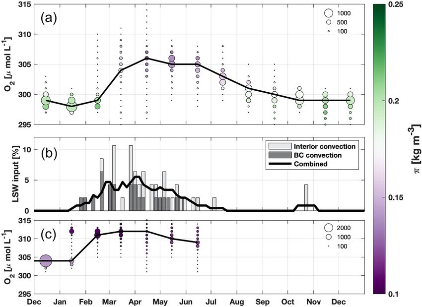
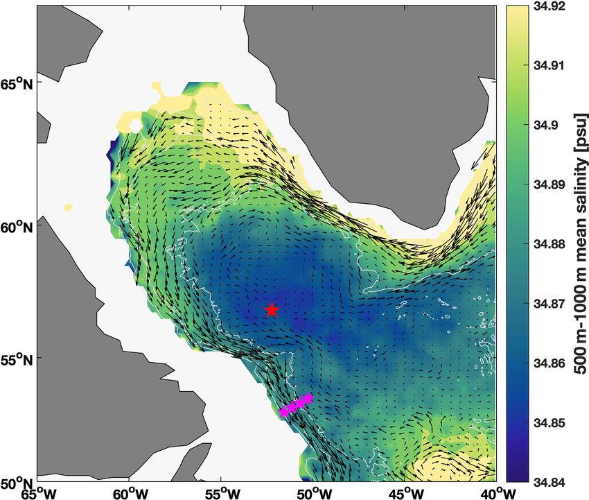
444                                                                                        J. Koelling et al.: 53◦ N LSW oxygen export

Figure 6. (a) T –S properties at K9 at 15 min resolution for four consecutive 5 d periods during the initial oxygen increase in February. Colors
correspond to oxygen concentration. Potential density (σθ ) contours are drawn with a spacing of 0.025 kg m−3 , and solid black contours show
densities of σθ = 27.68 and σθ = 27.8 kg m−3 . Note changed axis ranges compared to Fig. 5. (b) Density measurements at K8 at 50 and
608 m nominal depth. Shading for 608 m values shows density ranges of ± 0.01 and ± 0.03 kg m−3 from the measured values.

but similar density (Flament, 2002). Spiciness is used here               the record, but the number of observations in the central bin
as a water mass index to quantify the relative contribution               decreases. Moreover, a smaller secondary peak emerges at
of the two endmember water masses, LSW and IW. Figure 8                   a concentration of 306 µmol L−1 , with lower mean tempera-
uses data from the K9 mooring, and results from all other                 ture and salinity values, and there is a wide spread of oxygen
moorings are discussed in the following section.                          concentrations measured, ranging from 297 to 315 µmol L−1 .
   Overall, the seasonal cycle is marked by a shift from wa-              This is consistent with the view that, at this time, the bound-
ter with lower oxygen and T –S properties closer to those of              ary current waters comprise non-ventilated water, as well
IW towards high-oxygen LSW, which is most prevalent in                    as patches of recently convected and ventilated LSW (see
the months of March–July. In January, the bulk of the mea-                Sect. 3.1).
surements at K9 show similar properties. The most abun-                      In the following months, the LSW peak becomes more
dant class of oxygen values is at 298 µmol L−1 , and the wa-              pronounced and replaces the class of higher temperature and
ter mass index shows higher temperatures and salinities, in-              salinity water with low O2 as the most abundant water mass.
dicative of IW most likely advected from upstream within                  In April, the most commonly measured O2 value is at its
the boundary current. There is little spread around this mean             annual maximum of 306 µmol L−1 . By May, the boundary
value, with almost all measurements falling in the range                  current has become more homogenized, as evidenced by the
of 297–301 µmol L−1 . In the month of February, measure-                  higher number of observations in the central O2 bin. With
ments showing water with oxygen concentrations around                     the increased input of newly formed LSW, the T –S prop-
297 µmol L−1 still make up the majority of values seen in                 erties are at the opposite end of the water mass index (π )

Biogeosciences, 19, 437–454, 2022                                                                https://doi.org/10.5194/bg-19-437-2022
J. Koelling et al.: 53◦ N LSW oxygen export                                                                                           445

                                                                          more resembling the properties of IW, before the cycle be-
                                                                          gins anew the following winter.
                                                                             Figure 9 compares the seasonal oxygen cycle at K9 from
                                                                          Fig. 8 to the seasonal cycle of LSW input into the bound-
                                                                          ary current, as well as a partial seasonal cycle at 500 m depth
                                                                          from the SeaCycler mooring in the interior of the basin (see
                                                                          Fig. 1 for location). The input of LSW into the boundary cur-
                                                                          rent is an average over all years from the float data used in
                                                                          Sect. 3.1 and is calculated using Eq. (1). The gray bars show
                                                                          the LSW input during each 5 d period resulting from con-
                                                                          vection within the boundary current and LSW entering the
                                                                          boundary current from the interior, and the black line shows
                                                                          the combined input. Overall LSW input begins to increase
                                                                          in late January, peaks in April, and vanishes in July except
                                                                          for an isolated instance later in the year. Only 47 floats from
                                                                          the dataset measure LSW input into the boundary current,
                                                                          which could result in some bias of our estimate relative to
Figure 7. Fraction of total profiles from Holte et al. (2017) database
with mixed layer depth (MLD) over 600 m. Grey contours show the           the true underlying variability. However, the timing is consis-
2000 and 3000 m isobaths, and the magenta line shows the 53◦ N            tent with related measures such as the amount of LSW leav-
array. Overlaid are the convection locations for each float measuring     ing the interior derived from measurements of layer thick-
convection as defined in Sect. 2.3, differentiating between floats that   ness (Yashayaev and Loder, 2016) and rates of boundary–
are not found in the boundary current within the same year (red           interior exchange inferred from heat content changes (Stra-
dots), those that do enter the boundary current (yellow squares),         neo, 2006), suggesting that the overall variability is captured
and those that are found in the boundary current in either January        despite the very limited number of data points. The curve has
or February (green diamonds).                                             a similar shape to the seasonal cycle of the most commonly
                                                                          measured O2 concentration at K9 for each month, shown as
                                                                          a black line in the top panel, but the two are shifted relative
                                                                          to one another. The O2 concentration maximum increases in
                                                                          March, reaches its peak in April, and then stays at a similar
                                                                          level until June, before starting to decrease in July and Au-
                                                                          gust, lagging the increase in LSW input by about 1–2 months.
                                                                          Typical current speeds in the boundary current at the depth
                                                                          of the sensors used here are on the order of 15 cm s−1 (Zan-
                                                                          topp et al., 2017), and the distance to the region where the
                                                                          interior convection area is closest to the 3000 m isobath and
                                                                          where boundary current convection is most frequent is about
                                                                          450 km (see Fig. 7). The timescale for LSW to arrive at the
                                                                          53◦ N moorings after entering the boundary current would
                                                                          therefore be about 35 d. This is consistent with the time lag of
                                                                          approximately 1 month between the seasonal cycle of LSW
                                                                          input and the O2 maximum time series at the K9 mooring.
Figure 8. Monthly histogram of oxygen from December 2016 to               The data therefore support the hypothesis that the increase
December 2017 at about 600 m depth at K9. Colors show the mean            in oxygen concentration at the exit of the basin is largely
spiciness of each O2 bin, with lower values corresponding to LSW          controlled by the rate of formation and subsequent export of
and higher values to IW (see text for definition).                        LSW.
                                                                             LSW input from convection that occurs directly within the
                                                                          boundary current precedes the outflow of LSW from the inte-
compared to December–February. After June, oxygen con-                    rior by about a month, supporting the qualitative assessment
centrations are beginning to decrease again, with a concur-               made in Sect. 3.1 that the initial arrival of newly ventilated
rent increase in T and S, indicative of a larger fraction of              LSW at 53◦ N is likely a result of boundary current convec-
IW. Only isolated instances of elevated oxygen concentra-                 tion. Overall, 45 % of the input (21 of 47 floats) is associ-
tions are observed at K9 by August and September as the                   ated with boundary current convection and 55 % (26 of 47
water at 600 m depth becomes warmer, saltier, and less oxy-               floats) with interior convection, with both contributing about
genated. In the autumn months, the signature of LSW has                   equally in March and April when overall LSW input is high-
all but disappeared, with water found at the mooring once                 est. However, due to the caveats of our method discussed in

https://doi.org/10.5194/bg-19-437-2022                                                              Biogeosciences, 19, 437–454, 2022
446 J. Koelling et al.: 53◦ N LSW oxygen export Figure 9. (a) Monthly histogram of oxygen from December 2016 to December 2017 at 610 m depth at K9, as in Fig. 8. The size of each circle corresponds to the number of observations, the black line shows the bin with the highest number of observations for each month, and colors show the mean spiciness of each O2 bin. (b) Climatological seasonal cycle of LSW input into the boundary current from float data in 5 d bins as a fraction of the total input of LSW over the year (Eq. 1). Gray bars show separately the input from boundary and interior convection in each 5 d bin, and the black line shows the combined input smoothed with a five-point running mean. (c) Monthly histogram of oxygen from December 2016 to July 2017 at 500 m depth for the SeaCycler mooring in the deep convection area in the interior of the basin. The size of each circle corresponds to the number of observations, the black line shows the bin with the highest number of observations for each month, and colors show the mean spiciness of each O2 bin. Sect. 2.3, these numbers should not be interpreted as a mea- as eddies and current meanders may play a crucial role in the sure of the LSW volume flux associated with the two sources. export of newly formed LSW. At the SeaCycler mooring, there are two distinct peaks in the oxygen histogram in January as the mixed layer reaches 3.3 Differences at the 53◦ N array the sensor depth and ventilates water that had not been in contact with the atmosphere since at least the previous win- Although the seasonal oxygen cycle at K9 discussed in the ter. In February, newly ventilated, high-oxygen LSW be- previous section is representative of the general picture along comes the most prominent water mass, and O2 remains el- the 53◦ N array, there are also some horizontal differences. evated until the end of the available record in June 2017. The four moorings that carry oxygen sensors are deployed The maximum oxygen concentration found in the interior in different parts of the boundary current system at the exit before January is 304 µmol L−1 , much lower than the maxi- of the Labrador Sea (Zantopp et al., 2017, their Fig. 1). mum values at 53◦ N during March–July, confirming that the The K9 mooring, discussed in the previous section, is situ- increased oxygen levels of the outflowing boundary current ated within the core of the Deep Western Boundary Current must be associated with recently ventilated water rather than (DWBC), which has only a weak velocity shear between 400 LSW formed in previous winters. and 2000 m. K7 sits over the continental shelf beneath the If the bulk of the LSW entering the boundary current from core of the Labrador Current, which is surface intensified and the interior originates in the center of the basin near the Sea- carries colder, fresher water of Arctic origin. The K8 sensors Cycler mooring, the shortest distance to the boundary current at 600 m depth are within the DWBC but closer to the bound- would be about 230 km. With a time difference of about a ary with the Labrador Current and can be within it when the month between the oxygen increase at SeaCycler and the in- currents are meandering. At all three of these moorings, the creased input of LSW from the interior into the boundary cur- flow is southward, with mean velocities over the deployment rent, this implies a mean advection speed of 9 cm s−1 . This period between −13 and −15 cm s−1 . In contrast, the K10 is much larger than the climatological advection speed in the mooring is at the boundary between the offshore edge of interior (see Fig. 1), suggesting that short-lived features such the DWBC and its northward recirculation. Over the deploy- Biogeosciences, 19, 437–454, 2022 https://doi.org/10.5194/bg-19-437-2022
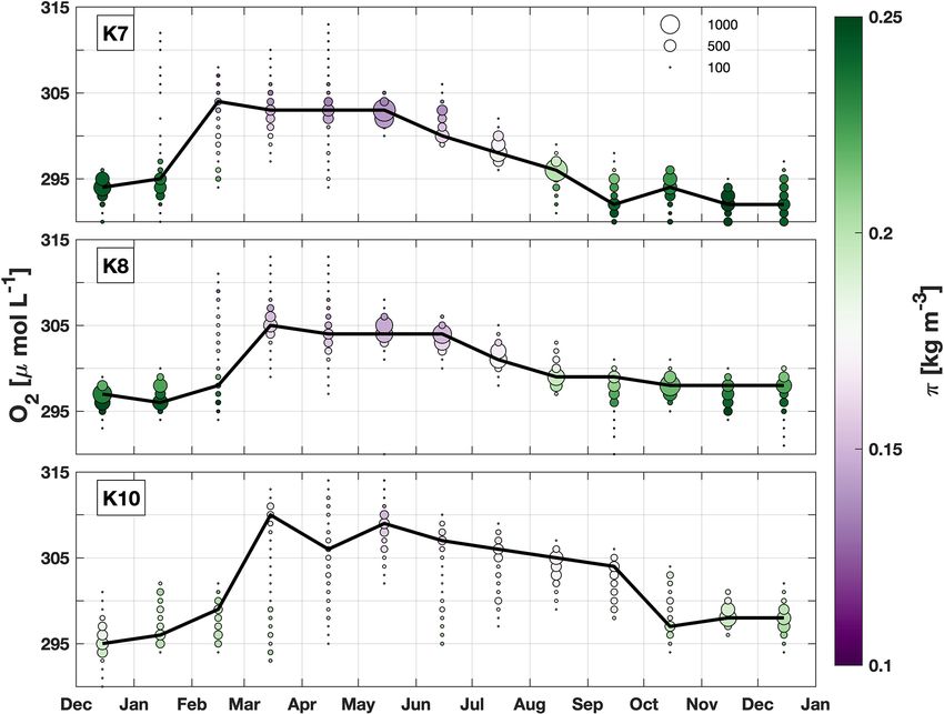
J. Koelling et al.: 53◦ N LSW oxygen export                                                                                         447

Figure 10. Monthly oxygen histograms, as in Fig. 8a, for the K7, K8, and K10 moorings. Circle size corresponds to number of observations,
the black line shows the bin with the highest number of observations for each month, and colors show the mean spiciness (π) in each bin,
highlighting the relative influence of IW and LSW.

ment period, there is a weak mean northward flow at about              of isopycnals steepening in winter over the continental slope.
600 m, with a speed of 3.5 cm s−1 , but daily mean values are          This weakened stratification may allow for the formation of
distributed evenly around this mean, ranging from −20 to               uLSW (Pickart et al., 1997). At K7, the highest oxygen con-
+20 cm s−1 . The seasonal cycle of oxygen concentrations at            centrations occur at lower densities and salinities, seen as a
all four moorings (Figs. 9a and 10) shows elevated values and          “tail” in the bottom left corner of the T –S plot. Moreover, the
water with properties closer to LSW during spring and sum-             first high-oxygen measurements occur almost 3 weeks earlier
mer, as well as water with lower oxygen values resembling              than at K9, which may suggest that these are a product of the
IW in autumn and winter.                                               formation of uLSW within the Labrador Current and that this
   At the border of the Labrador Current and DWBC, the                 formation takes place closer to the mooring section than the
oxygen concentrations measured at K8 show a similar sea-               production of classical LSW found at the other moorings.
sonal cycle as those at K9. Properties measured by the water           Since Argo floats generally stay offshore of the 2000 m iso-
mass index (π ) are also comparable, although the spread in            bath, formation of uLSW within the Labrador Current would
T and S is higher (Fig. 5), suggesting that the DWBC here is           be difficult to detect with the methods used in Sect. 3.1.
less homogenized than at K9.                                               At the offshore edge of the southward boundary current,
   Over the continental slope at K7, the oxygen concentra-             at mooring K10, the oxygen concentrations are more spread
tion is lower by about 5 µmol L−1 throughout the year, and             out, and elevated values are not found until the beginning of
the earliest arrival of elevated oxygen occurs in January com-         March. The spread of oxygen concentrations measured dur-
pared to February at K9. The water is generally warmer and             ing any given month is much larger than for the other moor-
fresher than at the other moorings, which may be the rea-              ings, and the T –S signature of the two different water masses
son for the lower oxygen values and also results in a slightly         is less pronounced. This is likely a result of current meanders,
lower mean density. There also seems to be a stronger sea-             with the mooring measuring the DWBC some of the time and
sonal variation in density compared to the other moorings.             its recirculation at other times, resulting in a wider range of
Between the warmer, saltier, oxygen-poor water in winter               ventilation histories. High oxygen concentrations are found
and the high-oxygen, low-T –S water in spring, density in-             during times of both southward and northward flow, suggest-
creases by more than 0.05 kg m−3 (Fig. 5). This is similar to          ing that LSW is carried southward with the offshore edge of
variability observed upstream in the boundary current near             the DWBC at K10, but some of it may also enter the north-
55◦ N by Cuny et al. (2005), who showed that this is a result          ward recirculation back towards the Labrador Sea.

https://doi.org/10.5194/bg-19-437-2022                                                            Biogeosciences, 19, 437–454, 2022
448                                                                             J. Koelling et al.: 53◦ N LSW oxygen export

4     Discussion                                                  tent with previous studies (Eden and Böning, 2002; Straneo,
                                                                  2006; de Jong et al., 2014).
4.1    LSW formation and export pathways                             In a recent study, Georgiou et al. (2020) used model data
                                                                  to analyze the source of water parcels reaching the 53◦ N
The analysis in Sect. 3.1 shows that deep mixed layers asso-      section, and they found that 41 % did not leave the bound-
ciated with convection are more commonly found in the inte-       ary current after passing Cape Farewell at the southern tip
rior. In Fig. 7, the area where more than 5 % of profiles mea-    of Greenland, while a further 44 % are modified in the inte-
sure mixed layers deeper than 600 m is about 15 times larger      rior of the basin before re-entering the boundary current, and
in the interior than inshore of the 3000 m isobath. However,      the remainder follow several less common pathways. These
this does not necessarily translate to 15 times larger oxygen     numbers are broadly consistent with the results from Fig. 8,
supply as water parcels have a longer residence time in the       with about equal amounts of LSW and IW found at the moor-
interior, whereas newly formed LSW in the boundary current        ings over an annual cycle. Our study suggests that there may
is rapidly exported (MacGilchrist et al., 2020, 2021). This       be a seasonal dependence to the split observed by Georgiou
is also evident in our data analysis, in which a significant      et al. (2020), with the LSW export (interior route) occurring
number of Argo floats measuring deep mixed layers in the          chiefly in the months after convection and IW (water from
interior do not enter the boundary current during the same        Cape Farewell) being more ubiquitous during autumn and
season and therefore do not directly contribute to the oxy-       winter. The input of newly ventilated LSW into the bound-
gen export by the outflowing boundary current. Moreover,          ary current in the months following convection observed here
LSW formation within the boundary current can also occur          is consistent with the more direct southward export of lighter
as slantwise convection (Cuny et al., 2005) or in parts of the    LSW found in their study, as well as results from an earlier
boundary current that are shallower than 2000 m, neither of       modeling study (Brandt et al., 2007). Georgiou et al. (2020)
which would be detectable with Argo floats. As discussed          suggested that pathways are different for the densest LSW
in Sect. 3.3, some evidence of convection over the continen-      formed in the interior, with water entering the boundary cur-
tal slope upstream can be seen in data from the K7 mooring        rent on the northern side of the basin and thus taking longer
at a water depth of 1400 m. However, neither the mooring          to reach 53◦ N. This density dependence may explain why
data, which do not measure local convection, nor the Argo         most of the LSW found in the mooring record seems to fol-
data, biased towards sampling regions with mild currents at       low the faster southward export route as the lower part of the
depth, provide sufficient information to quantitatively deter-    LSW layer is not sampled in the current sensor setup. An-
mine the portion of the LSW exported at 53◦ N that is formed      other model study by Handmann (2019) highlighted differ-
in the boundary current. The importance of boundary versus        ent routes that exist for LSW export, including several path-
interior convection for the outflowing LSW remains an open        ways for LSW entering the Irminger Sea. Their study also
question, with one previous estimate from float data conclud-     proposes that some of the water exported through the 53◦ N
ing that both could be important for the properties of the out-   section subsequently leaves the DWBC at Orphan Knoll near
flowing boundary current (Palter et al., 2008).                   50◦ N and recirculates back towards the north, reaching both
   Another crucial aspect concerning the export of LSW from       the Labrador and Irminger seas. In our data from the moor-
the formation region is how the water formed in the interior      ing furthest offshore, K10, there is evidence of high-oxygen
enters the boundary current. Palter et al. (2008) showed that     water with northward velocities (Sect. 3.3), suggesting that
both eddies and a mean cross-isobath flow can contribute to       newly formed LSW may also be entrained into this north-
LSW export, with floats entering the boundary current on all      ward recirculation.
sides of the basin, which is also the case for the float data        These studies show that many more LSW export pathways
used here (not shown). The timescale for a water parcel to        exist in addition to the direct southward route that seems
round the basin from Cape Farewell to the Labrador side           to be responsible for the pronounced seasonal signal at the
is about 147 d (Cuny et al., 2002). This implies that LSW         53◦ N moorings. Although the large summertime increase in
entering the boundary current, or formed within it, on the        oxygen (Fig. 8) is associated with LSW formed in the same
northern side of the basin during the height of convection in     year, the oxygen concentrations can also be impacted by ex-
March would not reach 53◦ N until August, when the influ-         port of LSW along these alternative routes, as well as fur-
ence of LSW at K9 is already decreasing. Thus, the outflow        ther water mass transformation along the pathway. For ex-
of LSW during summertime observed at 53◦ N is likely fed          ample, some of the LSW formed in the interior one year
mostly by LSW entering the boundary current on the west-          may be advected into the Irminger Sea, enter the boundary
ern or southwestern side, allowing for faster export out of the   current on the eastern side of Greenland, and stay within it
basin. The timing of the seasonal cycles of oxygen concen-        until it reaches 53◦ N several years later. Deep convection
tration in the interior, LSW input from the interior into the     also takes place in the Irminger Sea (de Jong et al., 2018),
boundary current, and oxygen concentration at K9 (Fig. 9)         leading to a somewhat weaker but still significant uptake of
implies that eddies may play an important role in exchang-        oxygen (Maze et al., 2012; Palevsky and Nicholson, 2018).
ing water between the boundary current and interior, consis-      The water mass formed by convection in the Irminger Sea,

Biogeosciences, 19, 437–454, 2022                                                    https://doi.org/10.5194/bg-19-437-2022
J. Koelling et al.: 53◦ N LSW oxygen export 449
known there as Irminger Sea Intermediate Water, or ISIW of 6 µmol L−1 at K9 during March–August 2017 relative to
(Le Bras et al., 2020), is mixed into the boundary current the January baseline of 298 µmol L−1 (Fig. 8) corresponds to
in the Irminger basin before it enters the Labrador Sea, af- an oxygen export of 1.37 ± 0.37 Tmol (1 Tmol = 1012 mol)
fecting the properties of what we have referred to here as for these 6 months. Over the whole year, the mean oxy-
Irminger Water (IW). Therefore, both the export of LSW into gen increase is 3.5 µmol L−1 , corresponding to an export of
the Irminger Sea and convection occurring there will have af- 1.60 ± 0.42 Tmol relative to the baseline value. With an in-
fected the properties of the ”low-oxygen” IW seen in Figs. 8– tegrated wintertime uptake across the air–sea interface due
10, and the annual minimum concentration of 298 µmol L−1 to gas exchange of 21.2 mol m−2 (Atamanchuk et al., 2020)
at K9 is likely already elevated compared to what it would and a convection area of approximately 150 000 km2 , the to-
have been without ventilation in the Labrador and Irminger tal uptake in the interior is 3.18 Tmol during the same year.
seas. Thus, about 43 % of the oxygen taken up during convection
is exported out of the basin via this fast export route of LSW
4.2 Global impact of Labrador Sea ventilation along the DWBC during summer and another 7 % through
slower export routes during the rest of the year. The good
Due to the global importance of LSW, it has long been as- agreement with the air–sea flux estimates from Atamanchuk
sumed that changes in its formation would play a crucial role et al. (2020) provides independent support for their notion
in setting the variability in the Atlantic Meridional Overturn- that bubble injection plays an important role in oxygen up-
ing Circulation (Koltermann et al., 1999; Yashayaev, 2007). take during deep convection. As discussed in Sect. 4.1, LSW
However, results from the Overturning in the Subpolar North is also exported along different pathways than we consid-
Atlantic Program (OSNAP) have called into question this ered here, and some remains in the basin until the next year,
long-held belief, showing that the bulk of the water mass which may account for the remaining 50 % of the oxygen up-
transformation across isopycnals occurs east of Greenland in take. Conversely, the recirculation of the DWBC towards the
the Irminger Sea and Iceland Basin. This water mass trans- formation region after it reaches Orphan Knoll (Fischer and
formation in the eastern section appears to be the main source Schott, 2002) may diminish the net oxygen export, although
of overturning variability (Lozier et al., 2019), although re- the recirculation strength is typically only about 10 % of the
cent modeling results suggest that LSW formation may still DWBC transport at 53◦ N (Zantopp et al., 2017).
be important for variability on multidecadal timescales that The deep North Atlantic is one of the few ocean re-
are not yet resolved by the OSNAP time series (Yeager et al., gions that has not experienced significant deoxygenation in
2021). recent decades (Schmidtko et al., 2017), with oxygen in-
In a recent follow-up study to the OSNAP results, Zou creasing slightly by about 1.7 Tmol yr−1 over their multi-
et al. (2020) showed that the disconnect between overturn- decadal study period compared to a globally integrated oxy-
ing and LSW formation is in large part due to density- gen loss of 70 Tmol yr−1 below 1200 m depth. The continued
compensated changes in temperature and salinity. Although formation and export of LSW and NADW may have con-
over 12 Sv of water mass transformation occurs in the tributed to staving off deoxygenation in this basin, and the
Labrador Sea from warm, salty waters to colder and fresher 1.60 Tmol yr−1 of export calculated for 53◦ N could be suf-
ones, the net transformation into the LSW density range is ficient to supply much of the oxygen consumed in the upper
only about 4 Sv. Our results are consistent with these find- NADW (uNADW) layer in the North Atlantic. Using a global
ings, showing that while the water mass properties of the out- mean apparent oxygen utilization rate of 0.1 µmol kg−1 yr−1
flow are altered substantially by the input of newly formed at 1500 m depth (Karstensen et al., 2008), an area of
LSW, its density remains largely unchanged. This suggests 26 159 000 km2 for the deep Atlantic Ocean between the
that LSW from the interior enters the boundary current pri- Equator and 50◦ N, and a mean layer thickness of 800 m for
marily along isopycnals, consistent with recent results from the isopycnal range 27.68 kg m−3 ≤ σθ ≤ 27.8 kg m−3 , we
models (Brüggemann and Katsman, 2019; Georgiou et al., estimate the annual oxygen consumption for this volume of
2020), with some along-isopycnal mixing occurring before water to be 2.2 Tmol yr−1 . If the depth-varying profile from
it reaches 53◦ N. Our time series also show for the first Karstensen et al. (2008) is used instead, with the depth range
time direct evidence that significant changes occur in the occupied by uNADW at each point estimated from density
oxygen content of the outflow, driven by the rapid export data, the estimate increases to 3.8 Tmol yr−1 . Using these
of newly ventilated LSW. While we only use data from a two estimates as a range of possible values for the annual
fixed depth, oxygen concentrations in the summer are ele- oxygen demand in this volume, the rapid southward export
vated in much of the LSW layer above 1200 m (Fig. 2). As- of LSW discussed here supplies 42 %–73 % of it, with the
suming that the oxygen input is comparable throughout this rest likely provided by slower export of LSW through other
layer, we can calculate a first estimate of the oxygen trans- routes, as well as uptake in other deep water formation re-
ported out of the basin due to the input of newly formed gions such as the Irminger Sea (Palevsky and Nicholson,
LSW: using a mean transport for the LSW layer at 53◦ N 2018), Iceland Basin (Maze et al., 2012), and the Gulf of
of 14.5 ± 3.8 Sv (Zantopp et al., 2017), the oxygen increase Lion in the Mediterranean Sea (Ulses et al., 2021). Thus, de-
https://doi.org/10.5194/bg-19-437-2022 Biogeosciences, 19, 437–454, 2022You can also read