Entertainment Demand from Expectations - Scott Kaplan Oskar Zorrilla December 31, 2022
←
→
Page content transcription
If your browser does not render page correctly, please read the page content below
Entertainment Demand from Expectations∗

                                                 Scott Kaplan†
                                                 Oskar Zorrilla‡

                                              December 31, 2022

                                                    Abstract

        This paper uses revealed preference methods to estimate demand for non-instrumental infor-
        mation in entertainment. We apply and extend the theory presented in Ely et al. (2015) to
        conduct an empirical analysis that examines the effect of suspense and surprise on consumer
        demand. We first introduce alternative definitions of suspense and surprise using the theory of
        mutual information, and prove that suspense is in fact expected surprise. We then estimate the
        impact of suspense and surprise on television viewership using play-by-play and high-temporal
        frequency television ratings data from the National Basketball Association (NBA). Our primary
        results suggest that a one standard deviation increase in suspense increases viewership by 2.53%
        - 2.91%, while surprise has no impact. We also estimate within-game impacts of (i) absolute
        score differential and (ii) absolute score differential with respect to the point spread on viewer-
        ship. These findings have important implications for entertainment media companies, including
        leagues and television broadcasters, and advertisers.

        Keywords: non-instrumental information, suspense, surprise, television viewership, NBA

   †
       Assistant Professor, Department of Economics, United States Naval Academy. email: skaplan@usna.edu.
   ‡
       Assistant Professor, Department of Economics, United States Naval Academy. email: zorrilla@usna.edu.
    ∗
      We would like to thank the Naval Academy Research Council and the Naval Academy Volgenau Fund for generous
financial support. We thank Cheenar Gupte for excellent research assistance. Special thanks to Ben Handel, Jim
Sallee, Sofia Villas-Boas, and David Zilberman for comments and inspiration. We’d also like to thank Nola Agha,
Anocha Aribarg, Max Auffhammer, Giovanni Compiani, Kwabena Donkor, Karl Dunkle-Werner, Claire Duquennois,
Gabe Englander, Alexander Frankel, Hal Gordon, Andy Hultgren, Benjamin Krause, Megan Lang, Brian Mills, Kate
Pennington, Jeff Perloff, Dan Putler, Gordon Rausser, Leo Simon, Avner Strulov Shlain, Steve Tadelis, Dmitry
Taubinsky, and Miguel Villas-Boas for thoughtful comments on this research. We’d also like to thank participants
in the United States Naval Academy Economics Seminar, UC Berkeley IO Seminar Series, the North American
Association of Sports Economics Annual Meeting, the Marketing Summer Research Series in the Haas School of
Business, the ERE Seminar Series at UC Berkeley, the NYU Stern Marketing Seminar Series, and participants at the
2022 Southern Economic Association Annual Meeting. Finally, special thanks to Ryan Davis for help in acquiring
the play-by-play data, and Todd Whitehead for useful feedback. All remaining errors are our own. © Scott Kaplan
& Oskar Zorrilla, 2023.

                                                         1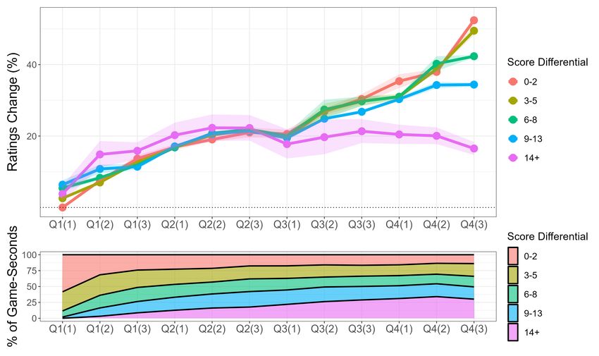
I   Introduction

Access to information is a crucial component of an economic agent’s decision-making process.

Information leading to such contingent actions is defined as instrumental. Instrumental information

applies to the entire spectrum of economic decisions, for instance how gas prices influence which

type of car to buy, how a sugar-sweetened beverage tax impacts soda consumption, or how wages

in a certain industry impact whether or not to change jobs. In particular, this information provides

additional certainty about a subsequent decision, which leads to welfare-improving actions, and

it is often the case that agents are willing to pay a premium for such information because of

the additional certainty it offers. In contrast, non-instrumental information does not have direct

consequences for economic decision-making under constraints, but provides utility nonetheless. For

instance, individuals may be attentive to the performance of candidates in a political debate, how

a television series will play out, or which team will prevail in a sporting event. In situations

featuring non-instrumental information, uncertainty over an outcome is itself a source of pleasure

for individuals.

   Most sources of non-instrumental information are found in entertainment settings, since the

uncertainty associated with the information is not associated with a financial stake. The global

entertainment media industry exceeds $2 trillion, and has grown 60% over the last 10 years (PWC

2019). Entertainment in its current form does not exist without well-crafted and targeted infor-

mation updating that attracts and keeps consumers’ attention. Additionally, provision of non-

instrumental information in certain entertainment settings has important social implications. The

ability to retain consumers through media outlets allows them to remain informed about important,

economically consequential issues.

   One can think of the outlay of non-instrumental information as the “thrill” associated with an

                                                                                                  2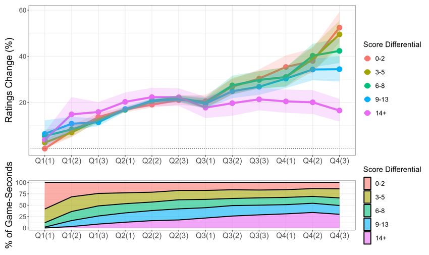
event. Thrill refers to adjustments in a spectator’s belief state as a result of new information about

an outcome. Ely et al. (2015) define two primary characteristics of thrill: suspense and surprise.

Higher suspense is defined as higher variance in future beliefs over an outcome, and higher surprise

is defined as a larger difference in current beliefs about an outcome compared to previous beliefs.

For instance, suppose a golfer is entering the final nine holes of a tournament in second place. There

is clear suspense over whether or not the golfer will prevail—beliefs are going to update relatively

soon given the approaching finality of the event. But on the 13th hole, the golfer drives the tee shot

into the water! This constitutes a significant change in the belief state about the golfer’s chances

to win.

   This paper uses revealed preference methods to explore and quantify demand for non-instrumental

information in entertainment, examining the “thrill” associated with the trajectory of an event.

We take as our starting point the definitions of suspense and surprise from Ely et al. (2015). We

propose alternative definitions based on information theory and show that suspense and surprise

are —both according to the Ely et al. (2015) and our own definitions— the same concept: suspense

corresponds to the ex ante flow of information while surprise corresponds to the ex post. We then

take both of our definitions as well as the theory presented in Ely et al. (2015) to conduct an

empirical analysis that examines the effect of thrill on consumer demand. We do so by leverag-

ing national 15-minute level viewership with play-by-play data for all games during the 2017-18

and 2018-19 seasons. Future work will rely on richer household-level second-by-second television

viewership data for all National Basketball Association (NBA) games during the 2021-22 season.

While there are many different avenues of entertainment to study non-instrumental information,

live sports is a natural application since (i) the suspense and surprise at any given moment of the

game is directly observed and publicly available, (ii) outcomes are plausibly random conditional

on an initial information state, unlike a book or movie, and (iii) because of the size of and value

                                                                                                    3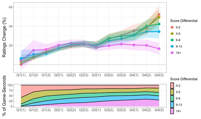
generated by the industry.

   Our empirical strategy employs conventional panel data methods to estimate a reduced form

model to determine the impact of suspense and surprise on total viewership, taking advantage of

the temporal granularity of our viewership and play-by-play data. Future work will estimate hetero-

geneous effects using household-level data that features demographic and geographic information.

We also plan to estimate a structural model of demand using each household’s viewership timeline

during the course of a game. That is, we observe the outside option faced by each household as

long as they tuned into a given game at some particular point (e.g. turning on a different game,

watching the news, turning the TV off, etc.), and use these switching events to infer a household’s

willingness-to-pay for thrill.

   The reduced form findings suggest that thrill is a large and significant factor affecting viewership

demand. Using the absolute score differential at different points in a game as a coarse measure of

thrill, we find that a one-point decrease in the absolute score differential does not impact viewership

in the first or second quarters, but increases viewership by 0.6% and 1.2% in the third and fourth

quarters, respectively, strongly supporting the hypothesis that viewers relish thrilling games, not

just games that are close. Contextualizing these results further, second half viewership is 8.2-20.5%

lower on average for games with a 14+ score differential compared to a 0-8 differential, while these

differences are 12.0-29.6% when only examining the fourth quarter.

   We extend this analysis to look at absolute score differential during a game in reference to the

closing point spread, similarly finding that viewership declines are starker towards the end of games.

I find that for every one-point increase in the score differential from the closing spread, viewership

declines by 0.1-0.9%, with larger decreases found in later stages of a game. This suggests that

a one-standard deviation change in score differential in reference to the spread during the final

quarter segment (9.3 points) exhibits an economically meaningful impact on viewership (6.4-7.3%

                                                                                                     4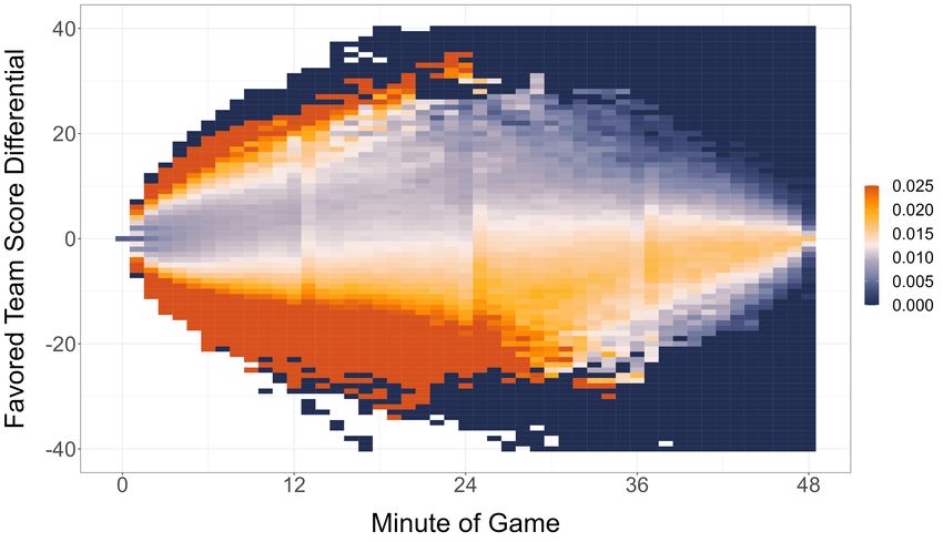
reduction), which amounts to roughly half the size of the impact of thrill over the absolute score

differential.

    Finally, we estimate the viewership response to the structural definitions of suspense and sur-

prise. Using the definitions of suspense and surprise from Ely et al. (2015), we find that a one

standard deviation increase in suspense increases viewership by 2.53%, while surprise has no statis-

tically significant impact on viewership. The results are quite similar using our proposed alternative

definitions of suspense and surprise: a one standard deviation increase in suspense increases viewer-

ship by 2.91%, while surprise again has no statistically significant impact. While these magnitudes

are seemingly small, suspense and surprise can take on an extremely large range of values. For

instance, in the last segment of the fourth quarter, a 0-2 point game experiences between 5.57-5.60

standard deviations more suspense than a 14+ point game. In this case, viewership would be

approximately 15.34-17.08% higher through suspense alone.

    The remainder of this paper proceeds as follows. First, we review the bodies of literature this

work is motivated by and contributes to in section II. Next, section III develops a conceptual frame-

work that introduces our alternate definitions of suspense and surprise and compares them with the

definitions provided in Ely et al. (2015). Section IV overviews the structure of the viewership and

play-by-play data and presents relevant summary statistics, including estimates of suspense and

surprise from the play-by-play data. Section V develops the set of reduced form empirical strategies

used in estimating viewership responses thrill. We present the results of the reduced form analysis

in section VI. Section VII proposes several additions we plan to implement in future work.

                                                                                                    5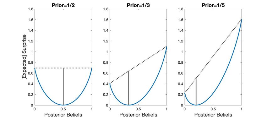
II   Literature Review

This research contributes to several notable bodies of literature. First and foremost, there is a

growing existing literature on suspense and surprise. Ely et al. (2015) is the seminal study that

provides the original definitions of suspense and surprise. They determine the optimal suspense

and surprise information policies that maximize expected utility. Their study incorporates practical

examples from entertainment and socially-relevant settings, including novels, political races, and

live sports. Preceding studies have also examined modified versions of suspense and surprise in a

theoretical manner and in various settings, including live sports (Bryant et al. 1994, Su-lin et al.

1997), game shows (Chan et al. 2009), and in the context of the Hangman’s Paradox (Geanakoplos

et al. 1989, Geanakoplos et al. 1996; Borwein et al. 2000). An adjacent literature uses laboratory

experiments to measure physiological responses to suspense and surprise, emphasizing that animals

are genetically driven to respond to such occurrences (Itti and Baldi 2009; Ranganath and Rainer

2003; Fairhall et al. 2001; Ebstein et al. 1996).

   To the best of our knowledge, there have been two peer-reviewed, empirically-oriented studies

to date using the suspense and surprise framework developed in Ely et al. (2015), and several other

working papers. Bizzozero et al. (2016) examine television viewership responses to suspense and

surprise over the course of tennis matches, finding that surprise, and to a lesser extent, suspense,

generate positive but relatively small viewership impacts. In particular, they find that a one stan-

dard deviation increase in suspense (surprise) raises audience viewership by 1,260 (2,630) viewers

per minute, which combine to cause a 3.65% viewership increase. They implement two separate,

but similar, methodologies to measure impacts of suspense and surprise: a Markov method and a

“betting odds” method, which uses live betting odds between each point during a match to dictate

outcome probabilities. Buraimo et al. (2020) examine television viewership in response to suspense

                                                                                                  6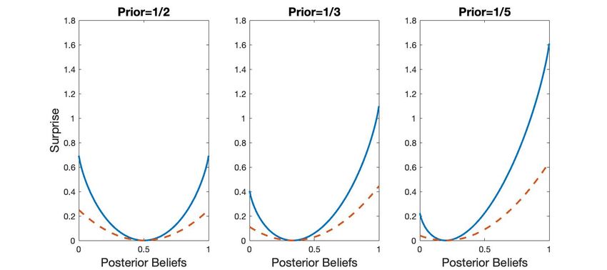
and surprise using the European professional football market. They also introduce “shock,” at each

portion of a match, which is defined as the difference between current outcome probabilities and

expected probabilities prior to the start of a match. Their findings also suggest relatively small

impacts of suspense and surprise on viewership; a one standard deviation in both suspense and

surprise increase audience viewership by 1.2%. Two recent working papers have assessed viewer-

ship responses to suspense and surprise in esport tournament streams (Simonov et al. 2020) and

professional baseball (Liu et al. 2020).

   This paper aims to extend the suspense and surprise literature in several key ways. First, we

introduce alternate definitions of suspense and surprise using the theory of mutual information,

which we apply in our empirical approach. Second, we examine an entirely different sport and

geographic market: professional basketball in the United States. There are notable differences

between the structure of basketball games and the settings studied in other related work, as well

as differences in the types of spectators watching games, which may lead to additional insights.

Next, we aim to take advantage of rich viewership and game play-by-play data to (i) estimate

both reduced form and structural models of viewership demand that account for household-level

demographic and geographic heterogeneity, and (ii) examine viewership responses to thrill over

alternative game outcomes (e.g. the point spread of a game), which may be unrelated to the final

outcome of who wins or loses. Finally, in future work we plan to use our empirical estimates of

viewership responses to thrill to assess the impact of a counterfactual game structures that can be

achieved through league rule changes.

   The second body of literature focuses on information preferences, which includes the theory of

addictive goods, and outcome resolution, formalizing the notion that individual taste preferences

are consistent with utility-maximizing behavior and may change over time (Stigler and Becker 1977;

Becker and Murphy 1988; Kreps and Porteus 1978; Caplin and Leahy 2001). We aim to expand

                                                                                                 7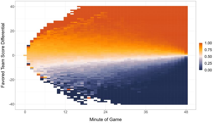
on this work by discussing and evaluating preferences for non-instrumental information, especially

in the context of outcome resolution. In particular, evaluating the psychological and emotional

attributes of entertainment is important in understanding the types of information individuals desire

(Fowdur et al. 2009). For instance, studies have shown that story “spoilers” have large impacts on

demand for entertainment goods, even suggesting that they have the potential to increase consumer

enjoyment (Leavitt and Christenfeld 2011; Johnson and Rosenbaum 2015; Levine et al. 2016; Ryoo

et al. 2020). Naturally, there has also been significant research assessing the impact of outcome

uncertainty on demand for live sports (Rottenberg 1956; Knowles et al. 1992; Humphreys and Miceli

2019; Alavy et al. 2010; Forrest et al. 2005).1 We extend this research by more closely examining the

evolution of beliefs over the course of an event, using random variation in event trajectories to assess

attention-based responses. This is particularly important as audiences increasingly explore real-

time gambling in live sports, which is likely to depend heavily on information relayed throughout

the course of an event (Kaplan and Garstka 2001; Haugh and Singal 2020; Salaga and Tainsky

2015).

       The third relevant body of literature is in hedonic pricing. Rosen (1974) provides a theoretical

framework that describes the total value of a good as a combination of the values of its attributes,

which has led to a rich body of literature applying the concept to a wide range of products (Busse

et al. 2013; Sallee et al. 2016; Currie and Walker 2011; Chay and Greenstone 2005; Luttik 2000).

This work focuses on an important attribute of entertainment goods - thrill. Television ratings

data is a natural avenue to explore impacts of these characteristics on consumer demand, as there

has been other work examining viewership responses to well-defined programming characteristics

(Fournier and Martin 1983; Anstine 2001; Livingston et al. 2013). Furthermore, there is existing

1
    It is important to note that while thrill and outcome uncertainty are related, they characterize different processes.
    Outcome uncertainty examines probabilities of different outcomes happening at different times, while thrill looks
    more fundamentally at the variance in the evolution of beliefs over the course of an event.

                                                                                                                       8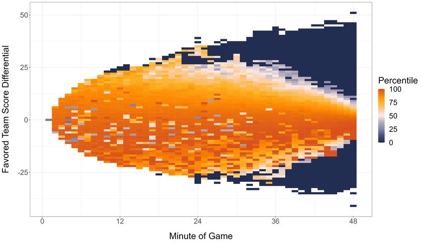
work using hedonic pricing methods in entertainment to understand the value of star performers,

which is highly related to the entertainment value generated by suspense and surprise (Scully 1974;

Kahn 2000; Rosen 1981; Hausman and Leonard 1997; Krueger 2005; Chung et al. 2013, Grimshaw

and Larson 2020; Kaplan 2020).

   The fourth and final body of literature is on the economics of advertising and consumer atten-

tion. Many forms of entertainment rely on advertising as a large source of revenue, and advertisers

themselves pay for the quantity and types of consumers the entertainment attracts (Becker and

Murphy 1993; Wilbur 2008; Bertrand et al. 2010; Hartmann and Klapper 2018). The stakes for

advertisers are quite high – analyzing time-use survey data, Aguiar et al. (2013) finds that the

average American spends about 20% of their time consuming some form of entertainment. The

evolution of thrill during the course of an event is paramount in generating spectator attention, and

this work aims to assess the extent to which each contributes to recruitment and retention of view-

ers. Furthermore, the type of information content used by advertisers in entertainment settings is

important for generating meaningful engagement with potential customers (Resnik and Stern 1977;

Bagwell 2005). In particular, there is a clear differentiation between informative content, which

corresponds characteristics like prices and deals, and emotional content, which corresponds to char-

acteristics like humor, slang, and emojis. Studies have shown that provision of emotional content

leads to higher levels of consumer engagement (Aaker 1997; Lee et al. 2018). In fact, Madrigal and

Bee (2005) find that the use of suspense as an advertising tactic is an important driver of consumer

attention. Using revealed preference methods to understand how consumers respond to thrill is

important in understanding how to better engage audiences with different advertising strategies.

                                                                                                   9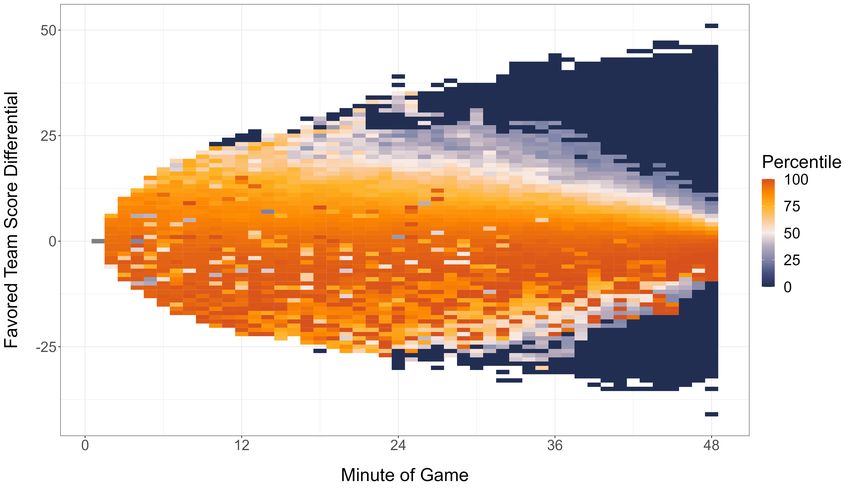
III   Conceptual Framework

Two opponents face each other in a match that is decided by the points scored — basketball, tennis,

football, among others — and a spectator watches in order to satisfy her desire to consume the

information flow that arises from the match. From the spectator’s vantage point the match can be

described as a stochastic process of beliefs. She approaches the match with an initial belief about

the eventual winner; as the clock ticks and the score differential changes so do her beliefs. In this

paper we will consider matches of this type with Bayesian spectators. While our framework applies

to any such match, our empirical focus will be on basketball.

A Beliefs

The state space in a match is binary, Ω ≡ {0, 1}, where, by convention, we let ω = 0 denote a

loss by the side initially favored to win. A belief at time t, bt , is a probability distribution over

outcomes bt ∈ ∆(Ω). Since Ω is binary, bt lies in the unit interval and is the probability at time t

that the initially favored side wins. A match of length T is a stochastic process γ ≡ {bt }Tt=0 .

Definition 1. A match, γ, is a stochastic process, {bt }Tt=0 , that satisfies the following conditions:

                    bt = Et [bt+1 ]                       (Dynamic Consistency)                 (III.1)

                    bt ∈ [0 1]                                      (Full Support)              (III.2)

                    b0 < 1                                           (Interesting)              (III.3)

                    bT ∈ {0, 1}                      (Resolution of Uncertainty)                (III.4)

   Condition III.3 makes the match worth watching to begin with; if the match is a foregone

conclusion, our spectator won’t watch it. Condition III.1 is the only requirement that Bayesian

                                                                                                     10
updating imposes on beliefs: it requires that γ is a random walk. Conditions III.2 and III.4
constrain the distributions, µ̃t , from which each innovation is drawn. It immediately follows that
the innovations to the random walk will not be drawn from identical distributions.
A Bayesian spectator’s beliefs will evolve according to the following law of motion:
bt+1 = bt + εt+1 , εt+1 ∼ µ̃t (III.5)
where µ̃t is a time-varying, mean zero, conditional distribution whose support is at most the unit
interval.
The two most crucial pieces of information are the margin and the time remaining: the point
differential and the time left to overturn that differential are the most straightforward determinants
of the outcome. Let δt denote the score advantage of the initially favored team at time t. Then bt
is the probability that the initially favored team (b0 > 1/2) wins conditional on δt while µ̃t is the
probability distribution over δt+1 conditional on δt .
B Preferences and Information
How does our Bayesian spectator evaluate the flow of information generated by the match? We
begin with the two concepts —suspense and surprise— developed by Ely et al. (2015). We offer
alternative definitions of these concepts and show that suspense is, in fact, expected surprise.
Definition 2. Surprise is the Euclidean distance squared between the current belief vector [bt 1−bt ]
and the prior belief vector [bt−1 1 − bt−1 ].
(bt − bt−1 )2 + ((1 − bt ) − (1 − bt−1 ))2 (III.6)
11Surprise is a measure of how far current beliefs are from previous ones. Importantly, it is a
realization. For any current beliefs, there are many possible future beliefs, surprise is the distance
between two consecutive belief realizations. Since beliefs are functions and we are interested in
measuring the distance between them, we instead propose the Kullback-Leiber distance between
two functions. We propose this distance because it is the standard used to measure distances
between probability distributions. In information theory it is also known as Relative Entropy. This
is also the definition of surprise used by Itti and Baldi (2009).
Definition 3. Surprise is the Relative Entropy between current beliefs bt and prior beliefs bt−1 .
bt 1 − bt
bt log + (1 − bt ) log (III.7)
bt−1 1 − bt−1
While the two definitions imply differences in marginal surprise, they share some similarities.
For a given prior belief, bt−1 , both are convex functions of the posterior belief, bt , that reach the
same minimum of zero at the prior. When beliefs do not change there are no surprises, regardless
of how we define surprise.
Figure 1 plots both surprise functions for three different priors. At the point of maximum
uncertainty, when the prior is 1/2, changes in beliefs in either direction are equally surprising
under both definitions. Both functions are symmetric around 1/2. As the prior moves closer to
one of the edges further movement of beliefs towards that edge becomes less surprising. In other
words, the more likely a state is, the less surprising confirmatory evidence becomes. Movement of
beliefs in the opposite direction, by contrast, become more and more surprising. Surprise is the
ex post revelation of information: at any moment in time it is a single point on one of the curves,
given the prior belief. The curves themselves represent the ex ante surprises that are possible for
a given prior belief.
12Figure 1: Surprise as function of belief realizations for three given priors: 1/2 (far left), 1/3 (center),
and 1/5 (far right). Solid, blue curve is Relative Entropy. Dashed, red curve is Euclidean distance
squared.
The ex ante counterpart of surprise is suspense. Ely et al. (2015) define suspense as follows:
Definition 4. Suspense is the sum of the conditional variance of bt+1 , where the sum is taken over
states of the world. In the binary case of basketball we have:
X
µ̃t ((bt+1 − bt )2 + ((1 − bt+1 ) − (1 − bt ))2
(III.8)
We can rewrite suspense only in terms of the innovations of the belief process.
Proposition 1. Suspense is twice the variance of εt+1 .
13Proof.
X
µ̃t ε2t+1 + (−εt+1 )2
=
X
=2 µ̃ε2t+1
= 2σt2
Broadly, suspense is an expectation of how much beliefs will change. But since beliefs are
bounded, the higher εt+1 is, the closer bt+1 must be to the edges of the simplex– the less uncertain
the spectator becomes. To be more precise, suspense is measuring how much information the
agent expects to receive. We therefore propose an alternative definition of suspense as the expected
amount of information flow between two consecutive periods.
As we have discussed above, the relevant information in a match is time remaining and score
differential. Let x and y be two random variables with joint pdf f (x, y) and f (x), f (y), denote the
marginal pdfs. The mutual information measures how much information you learn about x if you
know y, on average and vice versa.
X f (x, y)
f (x, y) log (III.9)
x,y
f (x)f (y)
In our case, let x denote the state and y the score differential. The mutual information tells us,
on average, how much we find out about the outcome of the game, ω, upon observing a score
14differential δt+1 . We can rewrite (III.9) in terms of conditional, rather than joint probabilities:
X f (ω, δt+1 )
f (ω, δt+1 ) log
f (ω)f (δt+1 )
ω,δt+1
X f (ω|δt+1 )f (δt+1 )
f (ω|δt+1 )f (δt+1 ) log
f (ω)f (δt+1 )
ω,δt+1
XX f (ω|δt+1 )
f (ω|δt+1 )f (δt+1 ) log
f (ω)
δt+1 ω
X X f (ω|δt+1 )
f (δt+1 ) f (ω|δt+1 ) log
ω
f (ω)
δt+1
f (ω|δt+1 ) is the posterior probability of winning/losing upon observing the score differential in
period t + 1, which we have denoted bt+1 for winning and 1 − bt+1 for losing. f (ω) is the prior
probability of winning/losing, which is bt for winning and 1 − bt for losing. Technically bt conditions
on the entire history of score differentials up to time, t, {δj }tj=0 . Under Markovicity, however, the
current score differential is a sufficient statistic. And finally, f (δt+1 ) is the probability of each
possible future score differential. But each possible score differential must be associated with a
unique posterior. So f (δt+1 ) is the probability of each posterior, which we have denoted µ̃t . If we
expand the inner sum over the two outcomes of winning and losing and replace each f (·) with the
terminology we have defined so far we end up with the following definition for Suspense:
Definition 5. Suspense is the Mutual Information between ω and δt+1 .
X bt+1 1 − bt+1
µ̃t bt+1 log + (1 − bt+1 ) log (III.10)
bt 1 − bt
While our information theoretic definitions of suspense and surprise are well-behaved in the
15interior of the simplex, we have to take some care at the edge when uncertainty is fully resolved.
We have required the uncertainty is resolved by the end of the match, but have not ruled out that
uncertainty might be resolved before; physical limitations make it so that certain score differentials
simply cannot be overturned in the remaining time. Bayesian updating implies the edge of the
simplex is an absorbing state. If bτ = 0 then ∀j > 0, bτ +j = 0, and similarly if bτ = 1. After
uncertainty has been resolved, there cannot be any further information flow. Both suspense and
surprise going forward must be zero. This leads us to adopt the following two conventions based
on continuity: limx→0 log xx = 0 and limx→0 x log(x) = 0.
There is a close information-theoretic connection between suspense and surprise. Suspense
is the expected information flow between the current and next period. Surprise is the realized
information flow between the previous and current period. We formalize this connection in the
following theorem:
Proposition 2. Suspense is expected Surprise.
The proof is fairly straightforward, so we include here.
Proof. We will prove it using both types of definitions. We begin with our definition. Iterate
expression (III.7) forward one period:
bt+1 1 − bt+1
bt+1 log + (1 − bt+1 ) log (III.11)
bt 1 − bt
This expression is the surprise at time t + 1. Of course, ex ante at time t there are many values
that (III.11) may take. Each value corresponds to a particular value of bt+1 and the probability of
16each is given by µ̃t . Therefore, the expected surprise is
X bt+1 1 − bt+1
µ̃t bt+1 log + (1 − bt+1 ) log (III.12)
bt 1 − bt
But this is simply the mutual information between ω and δt+1 . The proof using the Ely et al
definitions is identical.
Since the expectations operator is linear, the relationship between suspense and surprise can be
depicted geometrically. Consider figure 1. The future beliefs are on the horizontal axis. Whatever
the distribution of these possible future beliefs, its first moment must fall on the prior: 1/2, 1/3 or
1/5. We follow Kamenica and Gentzkow (2011) and depict this relationship geometrically in figure
2 for our alternative definitions of surprise and suspense.
While there are many possible values of suspense consistent with a prior belief, we are able to
bound those values. The minimum amount of suspense between two consecutive periods occurs
when the spectator knows, with probability one, that no new information will be revealed in the
following period. In that case, both the suspense and the surprise are zero. Notice that the surprise
functions in each of the three panels of figure 2 reaches its minimum value at the prior, or in this
case, the current belief. Zero information flow is equivalent to saying that beliefs do not change
and so this is the minimum amount of suspense possible.
The maximum amount of suspense between two consecutive periods occurs when the spectator
knows, with probability one, that the state will be fully revealed in the following period; once the
spectator knows the state of the world, she is fully informed. This means that only two posterior
beliefs are possible, zero or one. What is the distribution of these beliefs? Bayesian updating pins
down this distribution since it requires that its expected value is the prior. Since surprise is a
convex function, linearity of expectations implies that the suspense associated with this case lies
17Figure 2: Suspense for three given priors: 1/2 (far left), 1/3 (center), and 1/5 (far right). Solid,
blue curve is Relative Entropy. Dotted line is its convex closure. Vertical line segment represents
the suspense loci.
on the convex closure of the surprise function. Specifically, it is the point on the convex closure
that intersects with the prior belief. In figure 2 we depict the convex closure with a dotted line.
The resulting vertical line segment in each of the panels between zero and the convex closure is the
suspense locus for each of the three priors.
This result implies a type of observational equivalence between suspense and surprise in the
following sense: more suspenseful matches will, on average, yield more surprises. This means
that an econometrician might incorrectly conclude that a spectator likes surprise when in fact, she
likes suspense. We test this possibility in section V and report the results in Table 4. When we
regress viewership of basketball games on both suspense and surprise, only suspense is statistically
significant.
18C Alternative Outcomes
According to our definition of a match, γ, suspense and surprise occur with respect to the binary
outcome of winning/losing. Who wins need not be the only outcome of interest. Here we consider
two possible enrichments of the state space.
Within a match there are many intermediate outcomes that can elicit suspense, ex ante, and
surprise, ex post yet only marginally affect beliefs about which side will ultimately win. A player
who decides to take a shot from half-court can generate suspense among spectators as the ball flies
through the air.2 If the ball goes in, then spectators experience surprise: the ex post realization of
an ex ante low probability event has, by definition, a high information content (See the right-most
panel in figure 1).
It is also possible that the outcome of the match itself is not binary. Beyond the obvious fact
that in some matches draws are possible, the state space can be more general; just look at all of
the types of bets that can be placed around a given match. For a spectator who has placed a bet,
the relevant state space might, in fact, be the margin of victory. As Ely et al. (2015) show, it is
straightforward to generalize the state space from 2 to N dimensions. This applies to our definitions
as well. Both mutual information and relative entropy are well-defined for a an arbitrarily large,
discrete, state space.
Suspense and surprise over alternative outcomes is relevant for our empirical analysis, while the
case of most intermediate outcomes (e.g. the outcome of a single shot) are less so. The reason is
that moments within a game that generate suspense and surprise are too fleeting. It is not clear
why, on the margin, people might decide to tune in to a match — in our case, basketball — because
of the expectation that a rare play might be made, unless of course it is associated with a specific
2
This is actually one of the most tired tropes in sports films. When such a shot is taken, filmmakers underscore the
suspense by following the trajectory of the ball in slow motion.
19alternative outcome of interest (e.g. a bet over how many points a player may score in a game).
It is therefore unlikely that such moments would affect the consumption of information flow as
measured by TV ratings. The second enrichment, however, is less fleeting. If a consummate fan
has placed a bet on the score differential, suspense for her is not a function of who wins or loses,
rather, it is a function of the margin of victory.
IV Data and Summary Statistics
This section presents an overview of the data used in the analysis and the reduced form empirical
strategy. In the reduced form approach, we first estimate a coarse specification of the relationship
between suspense and surprise with viewership, relying on level changes in the absolute score
differential over the course of a game. We then estimate the viewership response to suspense
and surprise using the parameters defined in III, and separately repeat this estimation using the
suspense and surprise parameters defined in Ely et al. (2015).
A Overview of Data
There are two primary sets of data used in the analysis: (i) second-of-game play-by-play data
providing time-invariant information about each analyzed game as well as detailed information
about each moment of the game, and (ii) national 15-minute television viewership data for each
game from The Nielsen Company.3 Future work will leverage richer household-level data at the
second-by-second level, provided by FourthWall Media.
3
Data granted from The Nielsen Company (US), LLC. The conclusions drawn from the Nielsen data are those of
the researchers and do not reflect the views of Nielsen. Nielsen is not responsible for, had no role in, and was not
involved in analyzing and preparing the results reported herein.
20A.1 Play-by-Play Data
The play-by-play data spans the 2013-22 seasons, and includes both time invariant and time variant
information about each game. Relevant time invariant characteristics include the home and away
teams, time-of-day, network (local or the specific nationally-televised network), the initial point
spread, and an extensive list of team- and player-specific characteristics associated with each game.
the time variant data characterizes every “meaningful” action within a game, and is provided at a
second-of-play level.4 Most importantly, this data characterizes the real-time score at each second
of play a game, as well as a “wall clock” variable representing the time-of-day associated with each
observation. The last component is crucial, since it allows for accurate and precise merging of the
play-by-play data with the TV ratings data, which are denoted in time-of-day units.
A.2 Television Ratings Data
The second primary dataset used in this analysis is TV ratings data acquired from The Nielsen
Company.5 The data includes 15-minute interval ratings for every nationally televised NBA game
from the 2017-18 and 2018-19 seasons (including playoffs). The relevant metric for this analysis is
the projected total number of individuals watching during any given 15-minute interval.
B Summary Statistics
Table 1 presents a simple set of summary statistics spanning the two primary datasets. The table is
decomposed into Fixed-Game Characteristics and Within-Game Characteristics. The Fixed-Game
4
A non-exhaustive list of common occurrences warranting an observation include a made or missed basket, turnover,
foul, out-of-bounds stoppage, or timeout.
5
Data granted from The Nielsen Company (US), LLC. The conclusions drawn from the Nielsen data are those of
the researcher and do not reflect the views of Nielsen. Nielsen is not responsible for, had no role in, and was not
involved in analyzing and preparing the results reported herein.
21Characteristics provides information spanning 2013-22 coming from the play-by-play data, and
depicts the distribution of the absolute value of initial point spreads, total points scored in a game,
and the number of unique scoring events in a game. There are 12,765 games found in this sample.
We use this information to construct measures of suspense and surprise within games, which are
presented below.
Table 1: Summary Statistics
Mean SD Min Max N
Fixed-Game Characteristics (2013-22)
Point Spread 5.89 3.64 0 21.5 12,765
Total Points Scored 209.85 21.65 134 374 12,765
# of Scoring Events 145.79 11.84 103 198 12,765
Within-Game Characteristics (2017-19)
Total Viewership (1,000s) 2,683.29 2,460.62 265 20,956 4,771
Score Differential 8.14 7.02 0 53 58,771
Underdog Margin -2.79 10.38 -53 38 58,771
Consecutive Points 3.34 2.17 0 30 58,771
Real-Time Win Prob. Diff. 49.86 31.65 0 100 58,771
Note: The Fixed-Game Characteristics data is taken from play-by-play data across the 2013-22 seasons (both regular
season and playoffs). The 2013-22 data is used to calculate measures of suspense and surprise that are used in the
empirical analyses. The Within-Game Characteristics data includes only a subset of the play-by-play data, taken across
the 2017-19 seasons. The TV viewership data spans the 2017-19 seasons. Thus, the final column represents the number
of unique games from 2013-22 (12,765), the number of 15-minute viewership observations during the 2017-19 seasons
(4,771), and the total number of play-by-play events during the 2017-19 seasons (58,776).
The Within-Game Characteristics depicts information about events occurring within each game,
and only consists of play-by-play observations during the 2017-19 seasons. The first row represents
Total Viewership, which is observed at the 15-minute level within each game, amounting to 4,771
total observations. For these two seasons of data, we also provide distributions for score differen-
tial, underdog margin (defined as the average score differential between the favored team and the
underdog), consecutive points scored, and the real-time difference in win probability.
Figure 3 provides a heat map by favored team score differential and minute of game for a) the
22Figure 3: Win Probabilities and Standard Errors by Time and Score
a) Average Win Probabilities for Favored Team
b) Standard Errors of Outcome Probabilities for Favored Team
23average win probabilities for the favored team, and b) the standard errors of these win probabilities.
A high standard error suggests that there is relatively high variance in the win probability estimate
for that favored team score differential in that minute of the game. One can see that the highest
standard errors occur earlier in the game and for larger magnitudes in favored team score differential.
Figure 4: Suspense and Surprise by Time and Score
a) Ely, Frankel, and Kamenica Suspense b) Kaplan and Zorrilla Suspense
c) Ely, Frankel, and Kamenica Surprise d) Kaplan and Zorrilla Surprise
Finally, Figure 4 presents heat maps of the estimates of suspense and surprise by favored
team score differential and minute of game. We present estimates of suspense following the Ely
et al. (2015) definitions, which are presented in equations III.6 and III.8, as well as estimates
corresponding to our alternative definitions, depicted in equations III.7 and III.10. The heat maps
24show single percentiles of the suspense and surprise estimates. First, one can see in both the
EFK and KZ definitions there is a smoother gradient for adjustments in surprise compared to
adjustments in suspense. Intuitively, both suspense and surprise tend to be much higher in later
stages of a game when the score is relatively close. However, later stages of a game can also exhibit
the lowest levels of suspense and surprise when games feature scores that are not close. In earlier
stages of the game, suspense is significantly higher when the favored team trails the underdog,
which is also intuitive. Another important insight is that EFK surprise and KZ surprise appear
almost perfectly consistent with one another, in terms of percentiles. On the other hand, the heat
maps appear to differ more substantially in terms of suspense. This is a feature of the additional
convexity introduced by using the log-specification in the KZ definition of suspense, which results
in a distribution with higher variance. The standard deviation of EFK suspense is 0.0255 (mean:
0.0133), while the standard deviation of KZ suspense is 0.0345 (mean: 0.0199).
V Empirical Strategy
The empirical analysis in this section attempts to identify the impact of suspense and surprise on
television viewership. We first estimate a coarse specification of the relationship between suspense,
surprise, and viewership, examining heterogeneous impacts of level changes in the absolute score
differential by time remaining in the game. We expand on this by considering an alternative game
outcome: winning team with respect to the initial point spread. Finally, we estimate the viewership
response to suspense and surprise using the parameters defined in III, and separately repeat this
estimation using the suspense and surprise parameters defined in Ely et al. (2015).
25A Viewership Responses to Score Differential
We first analyze viewership responses using a directly observable game characteristic: absolute
score differential at each point during a game. Absolute score differential is the primary metric
by which a viewer internalizes suspense and surprise with respect to the final outcome of a game.
While it is inherently difficult to separate the notions of suspense and surprise using this metric
(since score differential at a given point can reflect both forward- and backward-looking beliefs), it
provides an intuitive understanding of how viewership responds to thrill over the course of a game.
As implied by the definitions in Section III, suspense and surprise are heavily dependent on time
remaining in an event, since this impacts the extent to which beliefs can change across periods.
Equation V.1 provides a general empirical model to measure viewership impacts in response to
observed absolute score differential and time remaining in an event.
Vjt = (Cjt ∗ Qjt )Λ + αj + ηt + ϵjt (V.1)
Vjt represents total viewership for game j at time-of-game t. Cjt denotes the specific game
characteristic impacting thrill (e.g. absolute score differential), and Qjt is a time-of-game indicator
(e.g. a minute of a game). Λ represents a vector of time-varying coefficients that reflect the impact
of Cjt on viewership. αj and ηt represent game and quarter-segment fixed effects, respectively.
One important distinction to make is the difference between a close game and a thrilling game.
A game featuring a low score differential in the first quarter would be characterized as close, but
not thrilling, since the variance in beliefs about the outcome probabilities in the next period is
low (suspense), and there was likely low variance in the evolution of beliefs prior to this point
(surprise).6 On the other hand, a low score differential in the fourth quarter would be considered
6
See Figure 4 for a visual depiction of this.
26both close and thrilling. Intuitively, the differential viewership impacts across the horizon of a game
for similar score differentials is the variation used to separate the impact of thrill on viewership
versus the impact of a close game.
We rely on Definition III.5 to interpret these estimates as plausibly causal, which stipulates that
beliefs over the final outcome update according to a first-order Markov process. Applying this to
the score differential itself, the realized absolute score differential in period t + 1, |Dt+1 |, is random
conditional on the score differential at time, |Dt |, and fixed information known prior to a game, b0 .
We believe a live sporting event to be an ideal setting in support this process.
|Dt+1 | ∼ N (|Dt |, σ 2 | b0 ) (V.2)
Figure 5 provides visual evidence in support of this assumption. It depicts the distribution
of the difference in the score differential at minute t versus minute t − 1. Thus, a difference of 0
implies that the score differential did not change between minute t − 1 and t. This figure suggests
Figure 5: Distribution of Difference in Score Differential at minute t and t − 1
27the evolution of the score differential from t − 1 to t follows a normal distribution centered around
0, which has important implications for spectator beliefs. From minute to minute, there is more
likely to be relatively small updating in beliefs than larger updating.
B Viewership Responses to Alternative Outcomes
Individuals may also experience suspense or surprise with respect to an outcome unrelated to which
team wins the game. Examples include which team covers the point spread, total points scored
over/unders, and other within-game propositions. The alternative outcome we examine empirically
is with respect to the point spread set before a game begins, which is one of the most common
measures gambled on by bettors. In this case, it is not the absolute score differential that determines
thrill, rather the absolute score differential in reference to the point spread.
The point spread is defined as the number of points PjT such that VjA + F (PjT ) = VjB , where
F (·) is a one-to-one function mapping points to strength.7 We index by T since point spreads
typically refer to E[DT ]. Using this setup, the absolute score differential in reference to the closing
point spread can be defined:
′
|Djt | = |Djt + PjT | (V.3)
where both Djt and PjT use the same team as the reference point for scoring. For instance, if
the home team is always used as the reference point, Djt > 0 implies the home team is leading,
and PjT > 0 implies the home team is an underdog. To understand this further, take the following
concrete example. Suppose there is a game featuring the Cleveland Cavaliers and Boston Celtics,
where the Cavaliers are the home team. If the closing point spread was -7, and the score at the end
of the third quarter was 85 - 82 favoring Cleveland, then the absolute score differential from the
7
Note that we index strength here at the game level, allowing for strength for a specific team to differ across games.
28spread would be equal to four. However, if the score was 85 - 82 in favor of Boston, the absolute
score differential from the spread would be equal to ten.
To measure thrill from this outcome, we rely on the methodology used in Salaga and Tainsky
(2015), who study television viewership for all PAC-12 football games from 2009-15. They examine
the impact of score differential during a game in reference to the closing point spread on average
television viewership for a game (they do not measure viewership changes over time within games).
The authors note that it is important to de-confound estimates from viewership corresponding to
the actual game outcome, represented by the raw score differential. To try and account for this,
the authors subset their analysis sample to i) the second half of games, ii) games with the absolute
score differential above some threshold level Gt=0.5T at halftime, and iii) games whose absolute
score differential does not fall below some threshold Gt>0.5T during the second half of a game.
One important difference in my approach is that we use real-time win probability estimates for
each game instead of absolute score differential to determine the subsample to study. This is because
a uniform score differential threshold may correspond to significantly different win probabilities in
different games. We set Gt=0.5T = 0.6 and Gt>0.5T = 0.4. Games must meet the criteria where at
halftime, the difference in win probabilities of each team winning is ≥ 0.6, and over the course of
the second half, that difference does not fall below 0.4. The results are not sensitive to restrictions
reasonably close to these bounds.
Applying this approach, we estimate a model of viewership in response to suspense over the
absolute score differential in reference to point spread as follows:
′
Vjt = (|Djt | ∗ Qjt )Λ + (|Djt | ∗ Qjt )Γ + αj + ηt + ϵjt (V.4)
s.t. |Pt=half time (A) − Pt=half time (B)| > Gt=0.5T & |Pt>half time (A) − Pt>half time (B)| > Gt>0.5T
29where all the terms maintain their previous definitions.
C Viewership Responses to Suspense and Surprise
Finally, we develop a reduced form model to jointly estimate the impacts of suspense and surprise on
viewership, as defined in section III. We perform two separate estimations: one using the definitions
of suspense and surprise provided in Ely et al. (2015) (definitions III.8 and III.6), and one using the
alternative definitions we propose (definitions III.10 and III.7). The general form of the estimating
equation is as follows:
Vjt = µXjt + ρYjt + αj + ηt + ϵjt (V.5)
Vjt represents total viewership for game j at time-of-game t. Xjt denotes the structurally defined
suspense parameter and Yjt the structurally defined surprise parameter. Game and time-of-game
fixed effects are denoted as αj and ηt , respectively. Therefore, µ and ρ represent the impacts of
suspense and surprise on viewership, respectively. As opposed to the previous estimations using
raw score differential, we can treat suspense and surprise as two different characteristics in this
estimation. The following section will present the results from each of the estimation approaches
discussed here.
VI Results
In this section we present three sets of results: (i) viewership responses during a game to the
absolute score differential, (ii) viewership responses during a game to the absolute score differential
with respect to the point spread, and (iii) viewership responses during a game to suspense and
surprise.
30A Viewership Responses to Score Differential
Table 2 shows two separate estimations. Column (1) presents a “naive” estimation, namely the
average impact of absolute score differential on log viewership. This specification is meant to
capture the average viewership response to score differential measured uniformly over a game (i.e.
a 2-point game in the first quarter is just as close as a 2-point game in the fourth quarter).8 Column
(2) differs from column (1) in that it presents the time-varying impacts of absolute score differential
on viewership, which corresponds to equation V.1.
Table 2: Impact of Absolute Score Differential on TV Ratings
Dependent Variable: log(Total Proj. Viewers Watching)
Absolute Score Diff. −0.0054∗ 0.0014
(0.0013) (0.0018)
Absolute Score Diff. * Q2 −0.0011
(0.0018)
Absolute Score Diff. * Q3 −0.0055+
(0.0023)
Absolute Score Diff. * Q4 −0.0118∗∗
(0.0027)
Game FE X X
Quarter Segment FE X X
Game + Quarter Segment Clusters X X
Observations 60,208 60,208
R2 0.9453 0.9471
Adjusted R2 0.9449 0.9466
Note: +
pdifferential reduces television viewership by 0.54%, and so close games are important in raising
viewership. Columns (2) shows a clear relationship between time remaining in the game and the
impact of score differential on viewership – a one point increase in absolute score differential in the
third and fourth quarters leads to an approximately 0.55% and 1.2% drop in viewership, compared
to a drop in the first two quarters that is not significantly different from zero. This is strong
evidence in support of the impact of thrill on viewership – marginal score differential changes
lead to higher viewership impacts when they lead to a larger variance in beliefs, either forward-
or backward-looking. As shown in Table 1, which depicts summary statistics of the play-by-play
data, the mean and standard deviation of absolute score differential are 8.14 and 7.02, respectively,
suggesting that viewership changes in response to changes in absolute score differential are quite
sensitive. Specifications are robust to clustering only at the game or quarter segment levels.
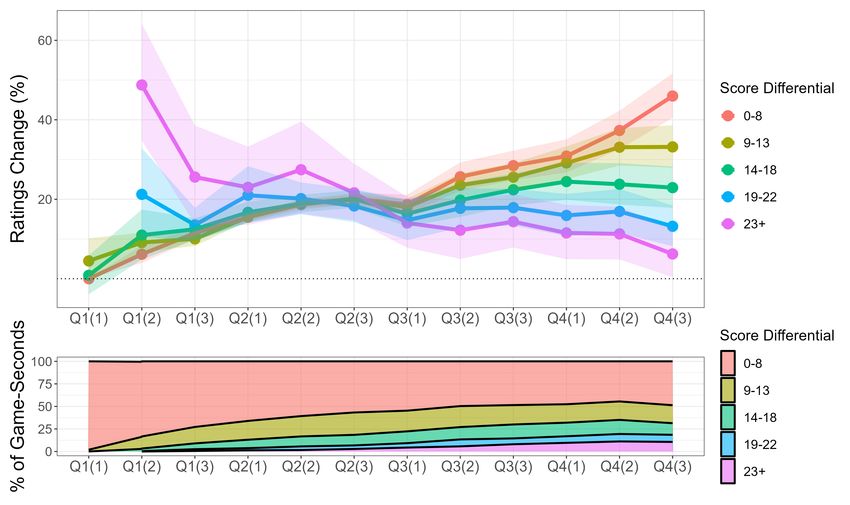
Figure 6 expands on Table 2 by examining the impacts of absolute score differential on view-
ership at a more granular level. We split each game into twelve equally long quarter segments,
and absolute score differential is divided into five bins using the quintiles of the distribution of
score differential in the data. All points in Figure 6 represent coefficients from an estimation tak-
ing the form of equation V.1, and can be interpreted as relative to the omitted score differential
bin-by-quarter segment (the 0-2 bin in the first quarter segment, Q1(1)).
First, this graph shows that average viewership over the course of a game is generally increas-
ing.Similar to Table 2, there are heterogeneous impacts of absolute score differential on viewership
as a game progresses to its later stages. While in the first half there are no significant differences
between each of the score differential bins and viewership changes, in the second half viewership
flattens out for the higher score differential bins compared to the lower bins. In particular, a game
in the closest absolute score differential quintile (0-2 points) features 8.2-20.5% lower viewership in
32Figure 6: Household Viewership Results by Score Differential Bin by Quarter Segment (%
Change)
the second half compared to a game in the largest absolute score differential quintile (14 + points),
with the difference increasing monotonically as a game approaches the end.
It is clear that the 14+ absolute score differential bin exhibits the most stark impacts on
viewership. Figure 7 examines these effects more closely, looking at the tails of the distribution
of absolute score differential. Here, impacts appear to be much more sensitive than those in the
primary support of the score differential distribution, where marginal increases in absolute score
differential when the differential is already quite high are much more impactful on viewership than
marginal increases when the differential is quite low. This effect is not only apparent towards
the end of games, but also for uncommonly large score differentials in the very early stages of
games, which would indicate heightened surprise. Estimations are robust to alternative clustering
33You can also read