FireFly: A Time Synchronized Real-Time Sensor Networking Platform
←
→
Page content transcription
If your browser does not render page correctly, please read the page content below
FireFly: A Time Synchronized Real-Time Sensor Networking
                            Platform
                        Anthony Rowe, Rahul Mangharam and Raj Rajkumar
                        Department of Electrical and Computer Engineering
                         Carnegie Mellon University, Pittsburgh, PA, USA
                                  {agr, rahulm, raj}ece.cmu.edu

1. Introduction
Networks of embedded wireless nodes provide a versatile platform for applications in industrial control, sur-
veillance and inventory tracking. Many of these applications are time sensitive in nature. For cost-effective
operation, such nodes feature low-power radios requiring data to be delivered across multiple hops over a
wireless interface to one or more destinations. In many applications, nodes must be battery-powered and
hence require energy efficient communication. In this chapter we will focus on using time synchronization
to provide real-time and energy efficient multi-hop wireless communication. Time synchronization enables
the construction of efficient and robust mesh networks for a large class of applications ranging from obser-
vation of sporadic events within sensor networks to real-time communication within tightly-coupled control
loops.

Time Synchronization in the wireless multi-hop domain provides the following benefits:
1. Energy Efficient Communication. An effective approach to energy-efficient service for applications
with either periodic or aperiodic flows is to operate all nodes at low duty cycles so as to maximize the
shutdown intervals between packet exchanges. Time synchronization is important because it tightly packs
the activity of all nodes so that they may maximize a common sleep interval between activities. Contention
based MAC protocols suffer from nearby nodes overhearing packets that are not addressed to them. In a time
synchronized network, nodes can be scheduled such that even though they could physically communicate
with each other, the topology is logically pruned to avoid it.
2. Bounded Message Latency. Time synchronization allows messages can be scheduled such that they
are collision-free. This provides guarantees on timeliness eliminating ambiguity about whether or not a
message was dropped or simply delayed. This is important for latency sensitive applications such as control
automation systems or interactive media streaming applications.
3. High Throughput. A tightly scheduled collision free environment allows for higher throughput than
a system using a contention based scheme. In the wireless sensor network setting this accommodates on-
demand bulk transfers of data such as firmware updates, logged sensor data or streaming of high data rate
sensors.
4. Deterministic Lifetime. The energy required to power sensor network radios is typically 10 to 20 times
more than the underlying CPU power. Since all communication is scheduled in advanced, time synchro-
nization enables the vast majority of energy consumption to be allocated in advanced. Later in the chapter
we will discuss how resource reservations can further refine the deterministic lifetime of these systems by
managing other energy consuming resources.
5. Total Event Ordering. Many applications such as localization and tracking require ordering of event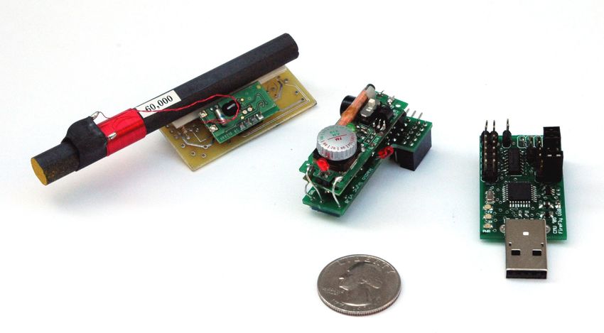
Power Energy
CPU (0.05mW ∗ tidle ) +
(24.0mW ∗ tactive )
Idle 0.05mW 0.05mW ∗ tidle
Active 24.0mW 24.0mW ∗ tactive
Network (.06mW ∗tidle )+(1.8uJ ∗
Nrx_bytes ) + (1.6uJ ∗
Ntx_bytes )
RX 59.1mW 1.8uJ per byte
TX 52.1mW 1.6uJ per byte
Idle .06mW .06mW ∗ tidle
Sensor
Light, Temp .09mW 11.25nJ per reading
Microphone 2.34mW 2.87uJ per reading
PIR 5.09mW 1uJ per reading
Accel 1.8mW 11.25nJ per reading
Table 1: Energy statistics for current hardware setup.
samples taken from different nodes at different times. Network wide time synchronization greatly simplify
this process by providing absolute time stamps that can be compared against each other.
FireFly is a platform with an accompanying software infrastructure that provides hardware assisted time
synchronization, a Time Division Multiple Access (TDMA) MAC protocol, RT-Link, for communication
and a reservation based real-time operating system (RTOS), nano-RK, for timely task processing. We have
successfully deployed the FireFly sensor platform in various environments. In particular we will discuss
our experiences deploying a network within a coal mine for location tracking as well as emergency voice
communication.
2. FireFly Hardware Platform
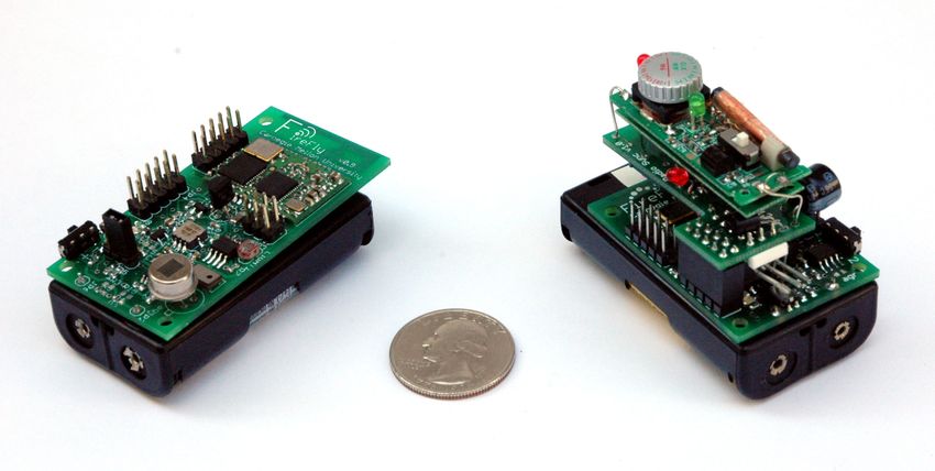
We developed a low-cost low-power hardware platform called FireFly as shown in Figure 1. The board
uses an Atmel Atmega32L [1] 8-bit microcontroller and a Chipcon CC2420 [2] IEEE 802.15.4 wireless
transceiver. The microcontroller operates at 8Mhz and has 32KB of ROM and 2KB of RAM. The FireFly
board includes light, temperature, audio, dual-axis acceleration and passive infrared motion sensors. We
have also developed a lower-cost version of the board called the FireFly Jr. that does not include sensors,
and is used to forward packets in the network or can be used as a module inside other devices such as
actuators that do not require sensing. The FireFly boards can interface with a computer using an external
USB dongle.
Table 1 shows a breakdown of the typical energy consumption of the different components on the FireFly
board. Since the transmit energy on the boards is quite low (1mW), the analog components in the radio’s
power amplifier are not as dominant as they would be in other forms of radio like 802.11. This accounts for
why the radio receive energy is greater than the transmit energy and means that nodes should not only try to
minimize packet transmission, but they should minimize listening time.
2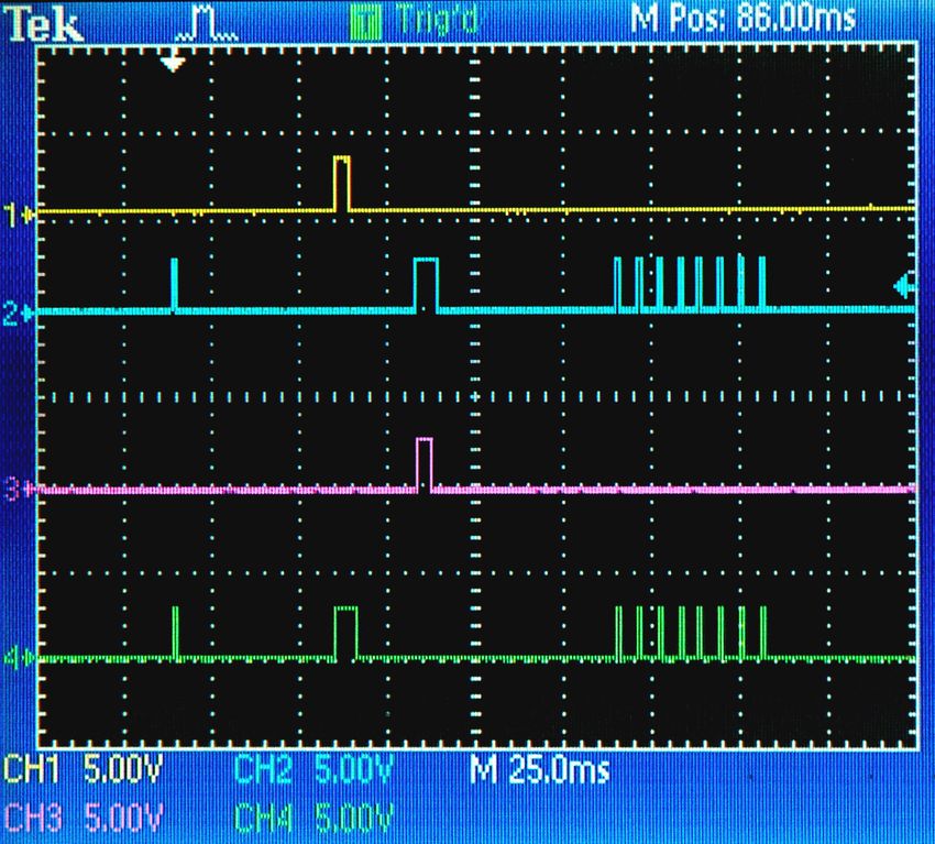
Figure 1: FireFly and FireFly Jr board with AM synchronization module

      Figure 2: Left to Right: WWVB atomic clock receiver, AM receiver and USB interface board.

2.1. Hardware Assisted Time Synchronization
In order to achieve the highly accurate time synchronization required for TDMA at a packet level granularity,
we use two out-of-band time synchronization sources. One uses the WWVB atomic clock broadcast, and
the other relies on a carrier-current AM transmitter. In general, the synchronization device should be low
power, inexpensive, and consist of a simple receiver. The time synchronization transmitter must be capable
of covering a large area.
    The WWVB atomic broadcast is a pulse width modulated signal with a bit starting each second. Our
system uses an off-the-shelf WWVB receiver (Figure 2) to detect these rising edges, and does not need to
decode the entire time string. When active, the board draws 0.6mA at 3 volts and requires less than 5uA
when powered off. Inside buildings, atomic clock receivers are typically unable to receive any signal, so
we use a carrier-current AM broadcast. Carrier-current uses a building’s power infrastructure as an antenna
to radiate the time synchronization pulse. We used an off-the-shelf low-power AM transmitter and power
coupler [3] that adhere to the FCC Part 15 regulations without requiring a license. The transmitter provides
time synchronization to two 5-storey campus buildings which operate on 2 AC phases. Figure 2 shows
an add-on AM receiver module capable of decoding our AM time sync pulse. We use a commercial AM
receiver module and then designed a custom supporting-board which thresholds the demodulated signal to
decode the pulse. The supporting AM board is capable of controlling the power to the AM receiver.
    The energy required to activate the AM receiver module and to receive a pulse is equivalent to sending
one and a half 802.15.4 packets. The use of a more advanced custom radio solution would bring these values
lower and allow for a more compact design. We estimate that using a single chip AM radio receiver, the
synchronization energy cost would be less then sending a single in band packet.
    In order to maintain scalability across multiple buildings, our AM transmitter locally rebroadcasts the
atomic clock time signal. The synchronization pulse for the AM transmitter is a line-balanced 50us square
wave generated by a modified FireFly node capable of atomic clock synchronization.
    We evaluated the effectiveness of the synchronization by placing five nodes at different points inside an

                                                     3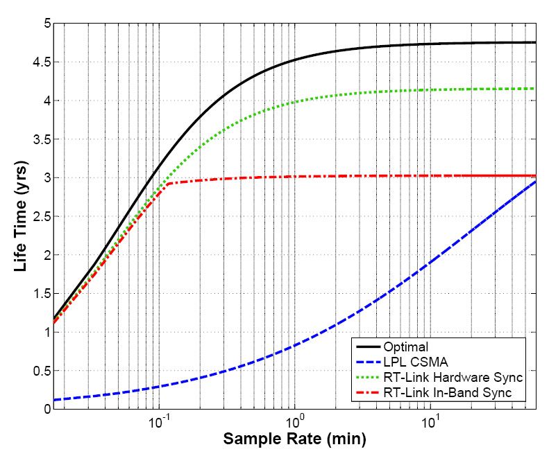
13.2
                                                                                                 node 0
                                                                                                 node 1
                                                       11.7                                      node 2
                                                                                                 node 3
                                                                                                 node 4
                                                       10.3

                           Percentage of Sync Pulses
                                                        8.8

                                                        7.3

                                                        5.9

                                                        4.4

                                                        2.9

                                                        1.5

                                                        0
                                                            0   50   100            150    200            250
                                                                     Time (microseconds)

      Figure 3: Distributions of AM carrier current time synchronization jitter over a 24 hour period.

8 story building. Each node was connected to a data collection board using several hundred feet of cables.
The data collection board timed the difference between when the synchronization pulse was generated and
when each node acknowledged the pulse. This test was performed while the MAC protocol was active in
order to get an accurate idea of the possible jitter including MAC related processing overhead. Figure 3
shows a histogram with the distribution of each node’s synchronization time jitter. An AM pulse was sent
once per second for 24 hours during normal operation of a classroom building. The graph shows that the
jitter is bounded to within 200us. 99.6% of the synchronization pulses were correctly detected. We found
that with more refined tuning of the AM radios, the jitter could be bounded to well within 50us.
     In order to maintain synchronization over an entire TDMA cycle duration, it is necessary to measure
the drift associated with the clock crystal on the processor. We observed that the worst of our clocks was
drifting by 10us/s giving it a drift rate of 10e-5. Our previous experiment illustrates that the jitter from AM
radio was at worst 100us indicating that the drift would not become a problem for at least 10 seconds. The
drift due to the clock crystal was also relatively consistent, and hence could be accounted for in software by
timing the difference between synchronization pulses and performing a clock-rate adjustment. In our final
implementation we are able to maintain globally synchronization to within 20us.

3. RT-Link: A TDMA Link Layer Protocol for Multi-hop Wireless Networks
RT-Link is a TDMA-based link layer protocol designed for networks that require predictability in through-
put, latency and energy consumption. All packet exchanges occur in well-defined time slots. Global time
sync is provided to all fixed nodes by a robust and low-cost out-of-band channel. We now describe in detail
the RT-Link protocol, packet types, supported node types and the protocol operation modes.

3.1. Current MAC Protocols
Several MAC protocols have been proposed for low-power and distributed operation for single and multi-
hop wireless mesh networks. Such protocols may be categorized by their use of time synchronization as
asynchronous, loosely synchronous and fully synchronized protocols. In general, with a greater degree of
synchronization between nodes, packet delivery is more energy-efficient due to the minimization of idle
listening when there is no communication, better collision avoidance and elimination of overhearing of
neighbor conversations. We briefly review key low-power link protocols based on their support for low-
power listen, multi-hop operation with hidden terminal avoidance, scalability with node degree and offered

                                                                           4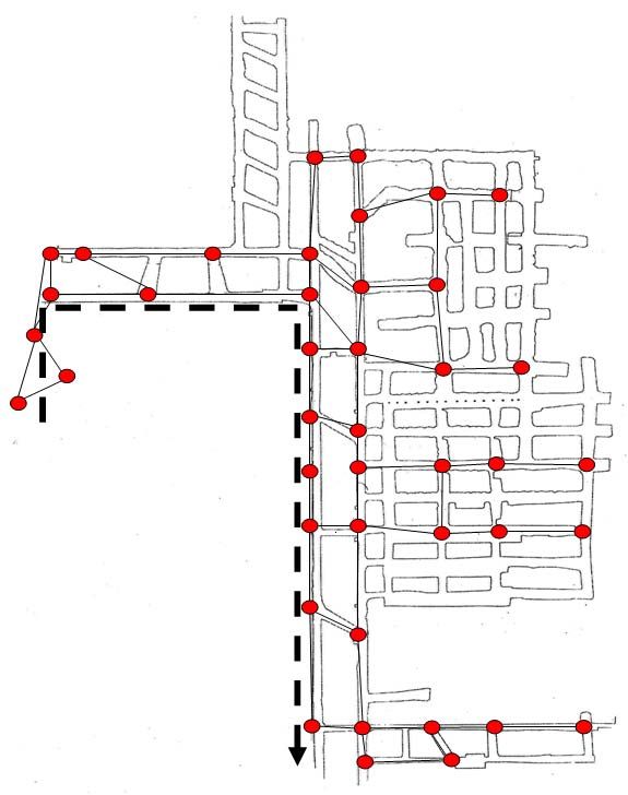
load.

3.1.1. Asynchronous Link Protocols
The Berkeley MAC (B-MAC) [4] protocol performs the best in terms of energy conservation and simplicity
in design. B-MAC supports carrier sense multiple access (CSMA) with low power listening (LPL) where
each node periodically wakes up after a sample interval and checks the channel for activity for a short
duration of 2.5ms. If the channel is found to be active, the node stays awake to receive the payload following
an extended preamble. Using this scheme, nodes may efficiently check for neighbor activity. For each
transmission instance, the transmitter must remain active for the duration of the receiver’s channel check
interval. This creates a major drawback since it forces the receiver to check the channel very often (in
milliseconds) even when the event sample interval spans several seconds or minutes. For example, if an
event occurs ever 20 minutes, all B-MAC receivers check the channel for activity approximately every 80ms
to limit the transmitter’s burst duration to 80ms [4]. This coupling of the receiver’s sampling interval and
the duration of the transmitter’s preamble severely restricts the scalability of B-MAC when operating in
dense networks and across multiple hops. B-MAC does not inherently support collision avoidance due to
the hidden terminal problem and the use of RTS-CTS handshaking with LPL is inefficient because the RTS
must use the extended preamble. In a multi-hop network, it is necessary to use topology-aware packet
scheduling for collision avoidance. Furthermore, upon wake up, B-MAC employs CSMA which is prone to
wasting energy and adds non-deterministic latency due to packet collisions.

3.1.2. Loosely Synchronous Link Protocols
Protocols such as S-MAC [5] and T-MAC [6] employ local sleep-wake schedules know as virtual clustering
between node pairs to coordinate packet exchanges while reducing idle operation. Both schemes exchange
synchronizing packets to inform their neighbors of the interval until their next activity and use CSMA prior
to transmissions. As all the neighbors of a node cannot hear each other, each node must set multiple wakeup
schedules for different groups of neighbors. The use of CSMA and loose synchronization trades energy
consumption for simplicity. WiseMAC [7], is an iteration on Aloha designed for downlink communication
from infrastructure nodes and has been shown to outperform 802.15.4 for low traffic loads. WiseMAC, how-
ever, does not support multiple hop communication. Both T-MAC and WiseMAC use preamble sampling to
minimize receive energy consumption during channel sampling. The use of CSMA in each scheme degrades
performance severely with increasing node degree and traffic.

3.1.3. Fully Synchronized Link Protocols
TDMA protocols such as TRAMA [8] and LMAC [9] are able to communicate between node pairs in
dedicated time slots. TRAMA supports both scheduled slots and CSMA-based contention slots for node
admission and network management. LMAC describes a light-weight bit-mask schedule reservation scheme
and establishes collision-free operation by negotiating non-overlapping slot across all nodes within the 2-hop
radius. Both protocols assume the provision of global time synchronization but consider it an orthogonal
problem. RT-Link has similar support for contention slots but employs Slotted-ALOHA [10] rather than
CSMA as it is more energy efficient with LPL. Furthermore, RT-Link integrates time synchronization within
the protocol and also in the hardware specification. RT-Link has been inspired by dual-radio systems such
as [11, 12] used for low-power wake-up. However neither system has been used for time synchronized
operation. Several in-band software-based time synchronization schemes such as RBS [13], TPSN [14] and
FTSP [15] have been proposed and provide good accuracy. In [16], Zhao provides experimental evidence
showing that over one-third of the population of immobile nodes in an indoor environment routinely suffer
a link error rate over 50% even when the receive signal strength is above the sensitivity threshold. This
severely limits the diffusion of in-band time sync updates and hence reduces the network performance.
RT-Link employs an out-of-band time synchronization mechanism which also globally synchronizes all

                                                      5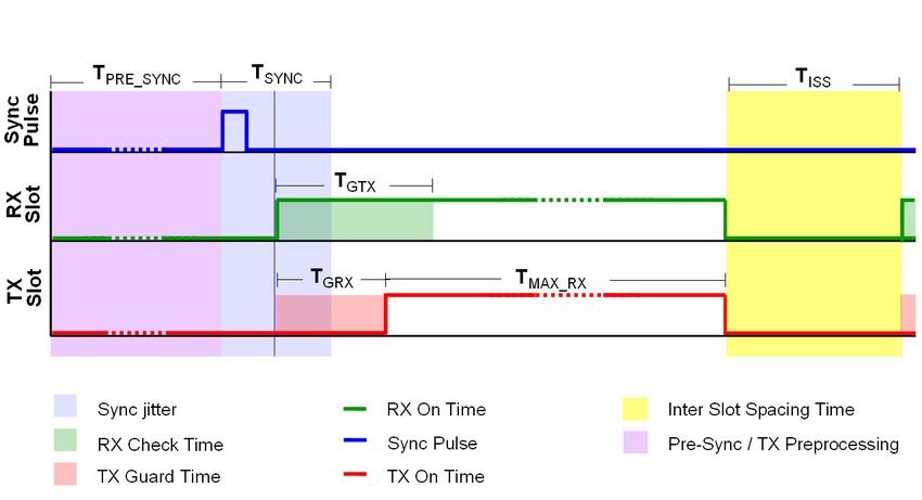
TDMA Cycle        Sync         Time-Sync Cycle
                                              Pulse

                                  Scheduled Slots              Contention Slots

              Figure 4: RT-Link time slot allocation with out-of-band synchronization pulses

nodes and is less vulnerable than the above schemes. We believe that hardware-based time sync adds new
properties to wireless sensor networks and warrants exploration in a practical environment.
     RT-Link supports two node types: fixed and mobile. Both node types include a microcontroller, 802.15.4
transceiver and multiple sensors and are described in detail in Section 2. The fixed nodes have an add-on
time sync module which is normally a low-power radio receiver designed to detect a periodic out-of-band
global signal. In our implementation, we designed an AM/FM time sync module for indoor operation and an
atomic clock receiver for outdoors. For indoors, we use a carrier-current AM transmitter [3] which plugs into
the power outlet in a building and uses the building’s power grid as an AM antenna to radiate the time sync
pulse. We feed an atomic clock pulse as the input to the AM transmitter to provide the same synchronization
regime for both indoors and outdoors. The time sync module detects the periodic sync pulse and triggers an
input pin in the microcontroller which updates the local time. As shown in Figure 4, this marks the beginning
a finely slotted data communication period. The communication period is defined as a fixed-length cycle and
is composed of multiple frames. The sync pulse serves as an indicator of the beginning of the cycle and the
first frame. Each frame is divided into multiple slots, where a slot duration is the time required to transmit a
maximum sized packet. RT-Link supports two kinds of slots: Scheduled Slots (SS) within which nodes are
assigned specific transmit and receive time slots and (b) a series of unscheduled or Contention Slots (CS)
where nodes, which are not assigned slots in the SS, select a transmit slot at random as in slotted-Aloha.
Nodes operating in SS are provided timeliness guarantees as they are granted exclusive access of the shared
channel and hence enjoy the privilege of interference-free and hence collision-free communication. While
the support of SS and CS are similar to 802.15.4, RT-Link is designed for operation across synchronized
multi-hop networks. After an active slot is complete, the node schedules its timer to wake up just before the
expected time of next active slot and promptly switches to sleep mode. In our default implementation, each
cycle consists of 32 frames and each frame consists of 32 5ms slots. Thus, the cycle duration is 5.12sec and
nodes can choose one or more slots per frame up to a maximum of 1024 slots every cycle. The common
packet header includes a 32-bit transmit and 32-bit receive bit-mask to indicate during which slots of a node
is active. RT-Link supports 5 packet types including HELLO, SCHEDULE, DATA, ROUTE and ERROR.
The packet types and their formats are described in detail in [17].

3.2. Network Operation Procedures
RT-Link operates on a simple 3-state state machine as shown in Figure 5. In general, nodes operating in
the CS are considered Guests, while nodes with scheduled slots are considered Members of the network.
When a fixed node is powered on, it is first initialized as a Guest and operates in the CS. It initially keeps
its sync radio receiver on until it receives a sync pulse. Following this, it waits for a set number of slots
(spanning the SS) and then randomly selects a slot among the CS to send a HELLO message with its node

                                                       6
Synchronize off of overheard packets

                                                                                      Guest
                                                                                   Synchronized

                                                      Got Scheduling Packet
                                                                                  Contention Mode

                                                                                                    Scheduling Conflict
                            Mobile
                        Unsynchronized
                        Contention Mode
                                                                                    Member
                                                                                   Synchronized
                                                                                  Scheduled Mode

                                   Figure 5: RT-Link node state machine.

ID. This message is then forwarded (via flooding if explicit routes are not present) to the gateway and the
node is eventually scheduled a slot in the SS. On the other hand, when a mobile node needs to transmit,
it first stays on until it overhears a neighbor operate in an SS. The mobile node achieves synchronization
by observing the Member’s slot number and computes the time until the start of the CS. Mobile nodes are
never made members because their neighborhood changes more frequencty and hence remain silent until a
Member provides it a time reference. All nodes with scheduled slots listen on every slot in the CS using
LPL. When a node chooses to leave the network, it ceases broadcasting HELLO packets and is gracefully
evicted from the neighbor list from each of its neighbors. The gateway eventually detects the absence of the
departed node from each of the neighbors’ HELLO updates and may reschedule the network if necessary.
     For fixed nodes that are unable to receive the global time beacon and for mobile nodes, RT-Link provides
software-based in-band time sync. Nodes can implicitly pass time synchronization onto another node using
the current slot in the packet header. This implicit time synchronization can cascade across multiple hops.

3.3. Logical Topology Control
RT-Link schedules communication based on the global network topology. This requires a topology-gathering
phase followed by a scheduling phase. In order to acquire the network connectivity graph, we aggregate the
neighbor lists from each node at the gateway. We then construct connectivity and interference graphs and
schedule nodes based on k-hop coloring, such that two nodes with the same slot schedule are mutually
separated by at least k+1 hops. Figure 6 shows the impact of node degree on lifetime. As the number of
neighbors a node communicates with increases, the number of transmit and receive slots correspondingly
increases consuming more energy. In Figure 7(a) we show the connectivity graph of a randomly generated
topology with 100 nodes. The graph was colored based on the connectivity to ensure that it is free of col-
lisions. Links can then be removed by instructing an adjacent node to no longer wakeup to listen on that
particular timeslot. Using this principle we can reduce the degree of nodes while checking to maintain net-
work connectivity. The reduced degree topology shown in Figure 7(b) reduces the average network energy
and simplifies routing. Such logical topology control is not possible with random access protocols.

3.4. Effectiveness of Interference-free Node Scheduling
A major underlying assumption in RT-link is that 2-hop scheduling results in an interference free schedule.
Traditionally, TDMA multi-hop wireless scheduling has been solved as a distance-k graph coloring problem,
where k is set to be 2. In order to validate this assumption, we tested the interference range of a node with
respect to its transmission range. We placed a set of nodes along a line in an open field and measured the
packet loss between a transmitter and receiver as the transmitter’s distance was varied. Once the stable
communication distance between a transmitter and receiver was determined, we evaluated the effect of a

                                                                              7
4.5
Degree 1
4
Degree 2
3.5
Degree 4
3
Lifetime (yrs)
Degree 8
2.5
2
Degree 16
1.5
1
0.5
0
0 0.5 1 1.5 2 2.5 3 3.5 4 4.5 5
Sampling Interval (min)
Figure 6: Life given increasing node degree between 1 and 10. Node degree one yields the longest life.
connect d3
(a) Physical Connectivity Graph. (b) Pruned Logical Connectivity.
81
No Jammer
0.9 RX−TX 2m
RX−TX 4m
RX−TX 6m
0.8 RX−TX 8m
RX−TX 10m
0.7
Packet Percentage
0.6
0.5
0.4
0.3
0.2
0.1
0
0 5 10 15 20 25 30
Distance (meters)
Figure 7: Packet Success rate while transmitting in a collision domain.
constantly transmitting node (i.e. a jammer) on the receiver. Our experimental results for stable transmission
(power level 8) are shown in Figure 7. We notice that 100% of the packets are received up to a transmitter-
receiver distance of 10m. Following this, we placed the transmitter at a distance of 2, 4, 6, 8, 10 and
12 meters and for each transmitter position, a jammer was placed at various distances. At each point, the
transmitter sent one packet every cycle to the receiver for 2000 cycles. We measure the impact of the jammer
by observing the percentage of successfully received packets.
We observe two effects of the jammer: First, the effect of the jammer is largely a function of the distance
of the jammer from the receiver and not of the transmitter from the receiver. Between 12-18 meters, the
impact of the jammer is similar across all transmitter distances. Second, when the transmitter and jammer
are close to the receiver, (i.e. under 9m), the transmitter demonstrates a capture effect and maintains an
approximately 20% packet reception rate.
The above results show that the jammer has no impact beyond twice the stable reception distance (i.e.
20m) and a concurrent transmitter may be placed at thrice the stable reception distance (i.e. 30m). Such
parameters are incorporated by the node coloring algorithm in the gateway to determine collision-free slot
schedules.
3.5. Network Scheduling
In multi-hop wireless networks, the goal of scheduling has often been to maximize the set of concurrent
transmitters in the network [18]. This is achieved either by scheduling nodes or links such that they operate
without any collisions. In the networks considered here, the applications generate steady or low data rate
flows but require low end-to-end delay. In Figure 8 we see two schedules, one with the minimal number of
timeslots, the other containing extra slots but provisioned such that leaf nodes deliver data to the gateway
in a single TDMA cycle. The minimal timeslot schedule maximizes concurrent transmissions, but causes
quequeing delays and hence does not minimize the upstream latency of all nodes. By assigning the time
slots appropriately in preference to faster uplink and downlink routes, we note that for networks with delay-
sensitive data, ordering of slots should take priority over maximizing spatial reuse.
The generation of minimum delay schedules is similar to the distance-two graph coloring problem that
9G G
0 a 6 a
1 b 5 b
2 c d 3 3 c d 4
a g c d g e c d b a
0 e f 0 e h 2 e f 2 h f
1 g h 1 f b 1 g h 1
Figure 8: Maximal concurrency schedule (left) compared to a delay sensitive schedule (right). Note that the
maximal concurrency schedule needs two frames to deliver all data.
Left graph shows maximal concurrency that needs two
frames to deliver all data. Even if you duplicate the
schedule, you will require 2 extra cycles compared to the
left graph.
G G G
G
0 1 0 1 6 5
2 3 2 3 4 3
1 4 1 0 5 4 5 6 1 2 1 0
a) b) c) d)
Figure 9: Ordered Coloring to minimize upstream end-to-end delay.
0 7 0
Δ1 Δ2 Δ7 Δ1 Δ3 Δ5
1 6 3
Δ1 Δ2 Δ7 Δ1 Δ4 Δ4
2 5 7
Δ1 Δ2 Δ7 Δ1 Δ5 Δ3
0 4 4
Δ1 Δ2 Δ7 Δ1 Δ4 Δ4
1 3 0
Δ1 Δ2 Δ7 Δ1 Δ3 Δ5
2 2 3
Δ1 Δ2 Δ7 Δ1 Δ4 Δ4
0 1 7
Δ1 Δ2 Δ7 Δ1 Δ5 Δ3
1 0 4
down up down up down up
(Δ 7) (Δ 14) (Δ 49) (Δ 7) (Δ 28) (Δ 28)
(a) (b) (c)
Figure 10: Different schedules change latency based on direction of the flow
10is known to be NP-complete [19]. In practice, many heuristics can work well and result in a small constant
deviation from the optimal [19]. To illustrate the minimum-delay capability of RT-Link, we briefly discuss
one such heuristic to schedule a network where the traffic consists of small packets being routed up a tree to
a single gateway. The heuristic consists of four steps. The first step builds a spanning tree over the network
rooted at the gateway. Using Dijkstra’s shortest path algorithm any connected graph can be converted into
a spanning tree. As can be seen in Figure 9(b), the spanning tree must maintain "hidden" links that are not
used when iterating through the tree to ensure the 2-hop constraint is still satisfied in the original graph.
Once a spanning tree is constructed, a breadth first search is performed starting from root of the tree. The
heuristic begins with an initially empty set of colors. As each node is traversed by the breadth first search,
it is assigned the lowest value in the color set that is unique from any 1 or 2-hop neighbors. If there are no
free colors, a new color must be added into the current set. The next step in the heuristic tries to eliminate
redundant slots that lie deeper in the tree by replacing them with larger valued slots. As will become apparent
in the next step, this manipulation allows data from the leaves of the tree to move as far as possible towards
the gateway in a single TDMA cycle. Figure 9(c) shows how the previous three nodes are given larger values
in order to minimize packet latencies. The final step in the heuristic inverts all of the slot assignments such
that lower slot values are towards the edge of the tree allowing information to be propagated and aggregated
in a cascading manner towards the gateway.
Many applications like interactive voice streaming may benefit from balanced upstream / downstream
latency. Figure 10 shows how different scheduling schemes can increase or decrease latency in a line for
each flow direction. Figure 10 (a) shows the minimum color schedule for a linear chain with a worst case
delay of 31 slots per hop, (b) shows the minimal upstream latency coloring optimized for sensor data col-
lection tasks with a minimum upstream delay of 1 slot, and (c) shows a balanced schedule for bi-directional
voice communication with a symmetric delay of 4 slots in either direction. Next to each node, is an arrow
indicating the direction of the flow and the number of slots of latency associated with the next hop. A change
from a lower slot value to a higher slot value must wait for the next TDMA frame and hence may have a
large penalty. We observe that for high end-to-end throughput, minimizing the number of unique slots is
essential. The minimum node color schedule in Figure 10 (a), delivers the maximum end-to-end throughput
for a chain of nodes assuming the TDMA cycle has only 3 colors, i.e. 1/3 the link data rate. Secondly, we
see that for delay-sensitive applications, ordering of the slots is just as important as minimizing the colors.
As seen in Figure 10 (c), we use many more colors, but achieve a lower end-to-end delay in both directions
then (a) which uses fewer colors.
3.6. Explicit Rate Control
RT-Link allows explicit rate control by specifying a 4-bit rate index r, in the schedule assigned to each node.
A flow’s rate is defined by the number of active frames that it transmits specified by 2r−1 . For example,
rate 1 transmits on every frame while rate 3 transmits on every 4th frame. Using this scheme we can vary a
flow’s rate by control the number of slots and the rate index assigned to it.
3.7. TDMA Slot Mechanics
When a node is first powered on, it activates the AM receiver and waits for the first synchronization pulse.
Figure 11 shows the actual timing associated with our TDMA frames. Once the node detects a pulse, it
resets the TDMA frame counter maintained in the microcontroller which then powers down the AM receiver.
When the node receives its synchronization pulse, it begins the active TDMA time cycle. After checking
its receive and transmit masks, the node determines which slots it should transmit and receive on. During
a receive timeslot, the node immediately turns on the receiver. The receiver will wait for a packet, or if no
preamble is detected it will time out.
The received packet is read from the CC2420 chip into a memory address that was allocated to that
particular slot. We employ a zero-copy buffer scheme to move packets from the receive to the transmit
11Figure 11: RT-Link operation and timing parameters.
queue. In the case of automatic packet aggregation, the payload information from a packet is explicitly
copied to the end of the transmit buffer. When the node reaches a transmit timeslot, it must wait for a
guard time to elapse before sending data. Accounting for the possibility that the receiver has drifted ahead
or behind the transmitter, the transmitter has a guard time before sending and the receiver preamble-check
has a guard time extending beyond the expected packet. Table 3 in the next section shows the different
timeout values that work well for our hardware configuration. Once the timeslot is complete, there needs to
be an additional guard time before the next slot. We provide this guard time plus a configurable inter-slot
processing time that allows the MAC to do the minimal processing required for inter-slot packet forwarding.
This feature is motivated by memory limitations and reduction of network queue sizes.
Figure 12 shows a sample trace of two nodes communicating with each other. The rapid receiver checks
at the end of the cycle show the contention period with low-power listening for the duration of a preamble.
3.8. Energy Model
To calculate the node duty cycle and lifetime we sum the node’s energy consumptions over a TDMA frame.
Table 2 shows the power consumed by each component assuming operation at 3 volts. Table 3 and Table 4
show the timing parameters and the energy of each operation during the TDMA frame. The active time of
each TDMA slot, Tactive , is dependent on the total number of slots, Nslots , the maximum slots transmit time
Tmax_payload , the AM synchronization setup Tsync_setup and capture Tsync as well as inter slot processing
time TISS . The number of slots and the length of the TDMA frame are dependent on the desired application
sampling rate and throughput configured by the developer.
Tactive = Tsync_setup + Tsync + Nslots ∗ (Tmax_payload + TISS ) (1)
The idle time, Tidle , between slots is the difference between the active time and the total frame time, Tf rame .
This is typically customized for the specific application since it has impact on both battery life and latency.
For long sampling intervals, idle time can be added at the end of the active TDMA slots.
Tidle = Tf rame − Tactive (2)
The three customizable parameters that define the lifetime of a node are the TDMA frame time, the number
of TDMA slots (including the number of contention slots Ncontention ) and the degree d of the node. As the
degree increases, the node must check the start of additional time slots and may potentially have to receive
packets from its neighbors. The minimum energy that the node will require during a single TDMA frame
Emin is the sum of the different possible energy consumers assuming no packets are received and the node
12Figure 12: Channels 1 and 2 show transmit and receiver activity for one node. Channels 3 and 4 show radio
activity for a second node that receives a packet from the first node and transmits a response a few slots later.
The small pulses represent RX checks that timed out. Longer pulses show packets of data being transmitted.
The group of pulses towards the right side show the contention slots.
does not transmit packets:
Emin = Esync + (d + Ncontention ) ∗ EGRX + ECP U _active
+ECP U _sleep + Eradio_idle + Eradio_sleep (3)
The maximum energy the node can consume during a single TDMA frame is the minimal energy consumed
during that frame summed with the possible radio transmissions that can occur during a TDMA frame.
Emax = Emin + (d + Ncontention ) ∗ ERX + NT X _slots ∗ ET X (4)
The maximum power consumed by a node over a TDMA frame can be computed as follows:
Pavg = Emax /Tf rame (5)
The lifetime of the node can be computed as follows:
Lif etime = (Ecapacity /Emax ) ∗ TF rame (6)
Figure 6 shows the lifetime of a single node with respect to the sample rate and the number of neighbors.
The node in this example is set to operate at the lowest rate that matches the sampling rate interval with
no contention slots. As the degree of the node increases, the number of receive checks increase hence
decreasing the lifetime. As mentioned before, logical pruning of the topology by selective listening can
have a large impact on system lifetime.
3.9. Lifetime
Two major factors control node lifetime in sensor networks are the topology and event sampling rate. We
have already shown how RT-Link allows for logical pruning of topology to conserve energy. We will now
investigate the lifetime with respect to event sampling rate. A typical LPL-CSMA approach must balance
long preamble transmit times with the frequency of channel activity checks. As described in [4] we observe
13Power Parameters Symbol I(ma) Power(mW)
Radio Transmitter Pradio_T X 17.4 52.2
Radio Receiver Pradio_RX 19.7 59.1
Radio Idle Pradio_idle 0.426 1.28
Radio Sleep Pradio_sleep 1e−3 3e−3
CPU Active PCP U _active 1.1 3.3
CPU Sleep PCP U _sleep 1e−3 3e−3
AM Sync Active Psync 5 15
Table 2: Power Consumption of the main components.
Timing Parameters Symbol Time (ms)
Max Packet Transfer Tmax_payload 4
Sync Pulse Jitter Tsync 100e−3
Sync Pulse Setup Tsync_setup 20 + (ρ ∗ Tf rame )
RX Timeout TGRX 300e−3
TX Guard Time TGT X 100e−3
Inter Slot Spacing TISS 500e−3
Clock Drift Rate ρ 10e−2 s/s
Table 3: Timing Parameters for main components.
Energy Parameters Symbol Energy (mW)
Synchronization Esync Psync ∗
(Tsync + Tsync_setup )
Active CPU ECP U _active PCP U _active ∗ Tactive
Sleep CPU ECP U _sleep PCP U _sleep ∗ Tidle
TX Radio Eradio_tx Pradio_tx ∗
(Tmax_payload + TGT X )
RX Radio Eradio_rx Pradio_rx ∗ Tmax_payload
Idle Radio Eradio_idle Pradio_idle ∗ Tactive
Sleep Radio Eradio_sleep Pradio_sleep ∗ Tidle
RX Radio Check EGRX Pradio_rx ∗ TGRX
Table 4: Energy of components with respect to power and time.
Optimal Check Interval (ms)
60 min
Life (yrs)
40 min
30 min
20 min
Check Interval (ms) Sampling Interval (min)
(a) LPL CSMA Check Rate vs Life at 30 min sample interval (b) Sample Interval vs Optimal Check Rate
Figure 13: Effect of Sample Interval on LPL CSMA Check Rate
14Lifetime (yrs)
Optimal
LPL-CSMA
RT-Link Hardware
RT-Link Software
Sampling Rate (min)
Figure 14: Sample Interval vs Lifetime for both CSMA and TDMA.
Parameter Symbol Value
Sleep Power Psleep 90mW
Sample Time Ts
Check Interval Tc
Channel Check Time Tcca 2.5ms
Sample Energy Esample 150mJ
Battery Capacity Cbat 2500mAh
Voltage V 3.0
Table 5: LPL-CSMA parameters.
a curve similar to Figure 13(a) where at a given sampling rate, there is an optimal lifetime produced by a
particular check rate. The authors in [4] neglected to include the voltage when calculating power and hence
their lifetimes where exaggerated. We show the corrected graph using power values based on our hardware.
The lifetime can be computed in (8).
Ts
Eidle = Psleep ∗ (Ts − (Tcca ∗ )) (7)
Tc
( TTsc ∗ Esample ) + (Tc ∗ Ptx ) + Erx + Ecpu + Eidle
L = Cbat / (8)
Ts ∗ V ∗ 24 ∗ 365
Table 5 describes the above values where L is the node lifetime in years. For a given sampling rate,
checking the channel more or less frequently can be quite inefficient. In a multi-hop environment, this
means that for a particular event rate of interest, the end-to-end latency is a function of the system check rate
which must be fixed in order to achieve the optimal lifetime. This implies that without time synchronization,
large sampling intervals will lead to longer latencies. Figure 13(b) shows the optimal check rate as a function
of the sampling rate. This is determined by taking the zero of the derivative of equation 8 for every sampling
rate. The dot represents the optimal check rate at the 30 minute sampling rate from the previous graph. Here
we see that even as the event rate approaches 100 minutes, the check rate must still be less than 4 seconds
150
1
.
.
G
.
n
Figure 15: Multi-hop network topology with hidden terminal problem.
7000
BMAC Adaptive 100ms
BMAC RTS/CTS 100ms
BMAC RTS/CTS 25ms
6000 BMAC Adaptive 25ms
RT−Link 300ms
RT−Link 1000ms
5000
Latency (ms)
4000
3000
2000
1000
0
1 2 3 4 5 6 7 8 9 10
Degree
Figure 16: Impact of Latency with node degree
to achieve the best lifetime. In that period of time with a single neighbor, approximately 1500 checks would
have gone wasted. Figure 3.8 shows sampling rate with respect to lifetime for RT-link (with and without
hardware time synchronization), the optimal node lifetime and the optimal LPL-CSMA lifetime. The overall
optimal lifetime assumes perfect node synchronization meaning that the only energy to be consumed is the
minimum number of perfectly coordinated packet transmit and receives and the system idle energy. The
LPL-CSMA line represents the lifetime given the optimal check rate. We see that for fast sampling rates,
hardware time synchronization makes less of a difference. This is because synchronization can be achieved
by timing the arrival of normal data messages that already contain slot information. As the sampling rate
increases, extra messages must be sent to maintain in-band time synchronization. We see that across the
range of a few seconds to nearly two hours, RT-Link with hardware synchronization is quite close to the
optimal lifetime and out performs the LPL-CSMA mac protocol by a significant margin.
3.10. End-to-end Latency
In order to investigate the performance of RT-Link, we simulated its operation to compare the end-to-end la-
tency with asynchronous and loosely synchronized protocols across various topologies. To study the latency
1612000
BMAC Adaptive 100ms
BMAC RTS/CTS 100ms
BMAC RTS/CTS 25ms
10000
BMAC Adaptive 25ms
RT−Link
8000
Packet Collisions
6000
4000
2000
0
1 2 3 4 5 6 7 8 9 10
Degree
Figure 17: Effect of node degree on collisions for B-MAC
in a multi-hop scenario we focused on the impact of the hidden terminal problem on the performance of
B-MAC and S-MAC. All the tests in [4] were designed to avoid the hidden terminal problem and essentially
focused on extremely low-load and one-hop scenarios. We simulated a network topology of two "backbone"
nodes connected to a gateway. One or more leaf nodes were connected to the lower backbone node as shown
in Figure 15. Only the leaf nodes generated traffic to the gateway. The total traffic issued by all nodes was
fixed to 1000 1-byte packets. At each hop, if a node received multiple packets before its next transmission,
it was able to aggregate them up to 100-byte fragments. The tested topology is the base case for the hidden
terminal problem as the transmission opportunity of the backbone nodes is directly affected by the degree
of the lower backbone node.
We compare the performance of RT-Link with a 100ms and 300ms cycle duration with RTS-CTS enabled
B-MAC operating with 25ms and 100ms check times. The RTS-CTS capability was implemented as outlined
in [4]. When a node wakes up and detects the channel to be clear, RTS and CTS with long preambles are
exchanged followed by a data packet with a short preamble. We assume B-MAC is capable of perfect clear
channel assessment, zero packet loss transmissions and zero cost acknowledgement of packet reception.
We observe that as the node degree increases (Figure 16), B-MAC suffers a linear increase in collisions,
leading to an exponential increase in latency. With a check time of 100ms, B-MAC saturates at a degree of
4. Increasing the check time to 25ms, pushes the saturation point out to a degree of 8. Using the schedule
generate by the heuristic in Section 3.5, RT-Link demonstrates a flat end-to-end latency.
The clear drawback to a basic B-MAC with RTS-CTS is that upon hidden terminal collisions, the nodes
immediately retry after a small random backoff. To alleviate problem, we provided nodes with topology
information such that a node’s contention window size is proportion to the product of the degree and the
time to transmit a packet. As can be seen in Figure 17, this allows for a relatively constant number of
collisions since each node shares the channel more efficiently. This extra backoff, in turn increases latency
linearly with the node degree. We see that RT-Link suffers zero collisions and maintains a constant latency.
174. Nano-RK: A Resource Centric RTOS for Sensor Networks
The push provided by the scaling of technology and the need to support increasingly complicated and diverse
applications has resulted in the need for traditional multitasking operating system (OS) abstractions and pro-
gramming paradigms. The case for small-footprint real-time OS support in sensor networks is strengthened
by the fact that many sensor networking applications are time-sensitive in nature i.e. the data must be
delivered from the source to the destination within a timing constraint. For example, in a surveillance ap-
plication, data relayed by a task which is responsible for detecting intruders and subsequently alerting the
gateway nodes of the system should be able to reach the gateway on a timely basis. In this section, we
present NanoRK, a small-footprint embedded real-time operating system with networking support.
NanoRK supports the classical operating system multitasking abstractions allowing sensor application
developers to work in a familiar paradigm resulting in small learning curves, quicker application develop-
ment times and improved productivity. We show that an efficient implementation of such a paradigm is
practical. We associate tasks with priorities and support priority-based preemption i.e, a task can always be
preempted by a higher-priority task that becomes eligible to run. For timing sensitive applications, we use
priority-based preemptive scheduling to implement the rate-monotonic paradigm [20] of real-time schedul-
ing so that a periodic sensor task set with timing deadlines can be scheduled such that their timing guarantees
are honored. Since modern sensor networks use ad-hoc multihop wireless networking for packet relaying,
we provide port-based socket abstractions that can be used by sensing tasks for sending and receiving data.
Since sensor nodes are resource-constrained and energy-constrained, we provide functionality whereby
the operating system can enforce limits on the resource usage of individual applications and on the energy
budget used by individual applications and the system as a whole. In particular, we implement CPU reser-
vations and Network Bandwidth reservations wherein dedicated access of individual application to system
resources is guaranteed by the OS. The OS also implements sensor reservations to enforce usage on the
number of accesses to individual sensors. Since the energy used by each task is the total sum of energy con-
sumed by the CPU, the radio interface and the individual sensors, a particular setting for each of these leads
to an energy reservation. Since we use a static design-time approach for admission control, we provide tools
for estimating the energy budget of each application and (hence) the system lifetime. The CPU , network
and sensor reservation values of tasks can be iteratively modified by the system designer until the lifetime
requirements of the node are satisfied.
4.1 Current Sensor Network Operating Systems
Infrastructural software support for sensor networks was introduced by Hill et al. in [21]. They proposed
TinyOS, a low footprint operating system that supports modularity and concurrency using an event-driven
approach. TinyOS supports a cyclic-executive model wherein interrupts can register events, which can then
be acted upon by other non-blocking functions. We believe that there are several drawbacks to this approach.
The TinyOS design paradigm is a significant departure from the traditional programming paradigm involving
threads, making it less intuitive for application developers. In contrast, we support a traditional multitasking
paradigm retaining task abstractions and multitasking. Unlike TinyOS, where tasks cannot be interrupted,
we support priority-based preemption. NanoRK provides timeliness guarantees for tasks with real-time
requirements. We provide task management, task synchronization and high-level networking primitives for
the developers use. While our footprint size and RAM requirements are larger than that of TinyOS, our
requirements are consistent with current embedded microcontrollers. Sensor network hardware typically
has ROM requirements of 32-64 KB and RAM requirements of 4-8 KB. NanoRK is optimized primarily
for memory and secondarily for ROM. SOS [22] is architecturally similar to TinyOS with the additional
capability for loading dynamic run-time modules. In contrast to SOS, we propose a static, multitasking
paradigm with timeliness and resource reservation support.
The Mantis OS [23] is the most closely related work to ours in the existing literature. In comparison to
18Mantis, we provide explicit support for periodic task scheduling that naturally captures the duty cycles of
multiple sensor tasks. We support real-time tasksets that have deadlines associated with their data delivery.
We use the novel mechanisms of CPU and network reservations to enforce limits on the resource usage of
individual tasks. With respect to networking we provide a rich API set for socket-like abstractions, and a
generic system support for network scheduling and routing. NanoRK is power-management and provides
several power-aware APIs that can be used by the system. 1
While low footprint operating systems such as uCOS and Emeralds [24] support real-time scheduling,
they do not have support for wireless networking. Our networking stack is significantly smaller in terms
of footprint as compared to existing implementation of wireless protocols like Zigbee (around 25 KB ROM
and 1.5 KB RAM) and Bluetooth (around 50KB ROM). We also provide high-level socket-type abstractions,
and hooks for users to develop or modify custom MAC protocols.
Our system infrastructure can be used to complement distributed sensor applications such as an energy
efficient surveillance system [25] and [26]. Our contributions are orthogonal to the literature on real-time
networking / resource allocation protocols [27, 28], energy-efficient routing/ scheduling schemes [29, 5] ,
data aggregation schemes [30], energy efficient topology control [31] and localization schemes [32, 33].
Our OS can be used as a software platform for building higher-layer middleware abstractions like [34]. Our
energy reservation mechanism can be used to prevent the type of energy DoS attacks described in [35].
Finally, our work complements [36] in extending the resource kernel paradigm to energy-limited resource-
constrained environments like sensor networks.
4.2. Design Goals for a Sensor Networking RTOS
We present the following design goals for an RTOS targeting wireless sensor networks.
• Multitasking: The OS should provide a simple and intuitive programming paradigm for easy use by
application developers. It is desirable to retain the traditional multitasking paradigm familiar to both
desktop and embedded system programmers. Application developers should be able to concentrate
on application logic rather than low-level system issues such as scheduling, and networking.
• Networking Stack Support: The OS should support multihop networking, routing and simple user-
level networking abstractions similar to sockets. In particular, low-level networking details such as
reliable packet transmission, multicasting, queue management etc. should be handled by the OS.
• Support for Priority-based Preemption: Node battery lifetime continues to be a major challenge in
sensor networks. Hence, given that energy consumed by processing per bit is significantly less than
the per-bit energy consumed by the radio interface, there is a trend toward increased local processing
(such as embedded vision and sound processing). This typically results in increased task execution
times. In such situations where task run-times are large, there is a need for priority-based preemption
to give precedence to higher priority events.
True preemptive multitasking becomes necessary in a system where multiple inputs to the system
must be serviced at different rates within a required period. For instance, imagine a sensing platform
consisting of a microphone, light sensor, radio interface, a GPS for position information or time
synchronization and a smart camera system. Figure Table 6 shows typical period and execution times
for each of these devices. Manually scheduling such a task set can become daunting using timer
interrupts.
A non-preemptive scheme might handle the radio with an external interrupt, the light and microphone
with two priority-based timers, and leave the GPS and camera processing for the main program loop.
Even in this situation, the developer may encounter difficulties because the camera servicing time
1
Power-aware APIs can also be used by applications, albeit with prudence.
19Period Execution Time
Radio Sporadic 10 ms
Microphone 200 hz 10 us
Light Sensor 166 hz 10 ms
Smart Camera 1 hz 300 ms
GPS 5 hz 10 ms
Table 6: A sample task set with update periods and execution times.
is longer than the period of the GPS. Given that many low-end microcontrollers have limited timer
interrupts, it can become difficult to schedule such a task set. Developers may need to resort to
manual time splicing of their functions, thus making future modifications difficult. With a preemptive
priority-based system, each of these sensing functions would be supported by a prioritized periodic
task.
• Timeliness and Schedulability: Most sensor applications such as surveillance tend to be time-
sensitive in nature where packets must be relayed and forwarded on a timely basis. While routing
and network link scheduling are important components in ensuring that packets meet their end-to-end
delay bounds, timing support on each node in the network is also essential. In order to honor end-to-
end deadlines, local tasks on each node have deadlines associated with the completion of their local
data relaying and processing. Managing the deadlines of these tasks requires support of a real-time
operating system.
• Battery Lifetime Requirements: Guaranteeing sensor node battery lifetimes of 3 to 5 years con-
tinues to be a major challenge in sensor networks. If limits on the usage of energy can be enforced,
lifetime guarantee requirements of the system as a whole can likely be provided (under reasonable
assumptions about operating conditions such as network connectivity). The OS can also ensure that
the system energy is apportioned in a manner commensurate to the importance of the tasks so that
critical tasks are guaranteed their energy budget.
• Enforcement of Resource Usage Limits: Since sensor nodes are resource-constrained, precious
CPU cycles, network buffers and bandwidth should be apportioned to application needs. OS support
for guaranteed, timely and limited access to system resources is necessary for supporting application
deadlines and balanced apportioning of system slack (residual unused resources). This mechanism
can also be used to place some limits on the impact of faulty or malicious tasks on system operation.
• Unified Sensor Interface Abstraction: Providing a unified and simple abstraction for accessing
sensor readings and actuating responses would greatly benefit the end-user. In particular, low-level
details associated with sensor/actuator configurations should be abstracted away from the user. Sen-
sors should be supported using device drivers that can return real-world units as well as raw ADC
values.
• Small Footprint: The current trend of low-end embedded processors is toward larger ROM sizes
(64KB to 128 KB) and smaller RAM sizes(2KB to 8KB). The OS architecture should be compliant
with this trend by optimizing for RAM with a higher priority than ROM and optimizing for runtime
efficiency. This memory constraint also implies that when the choice exists, one prefers a static
configuration to a dynamic decision that requires additional data storage and run-time manipulations.
20User Task User Task User Task
Real-Time Scheduler IPC
Task Peripheral
Management Drivers Network
Virtual Stack
Energy Reservations
Reservations
Kernel
Time Sync RX Power Control
Microcontroller 802.15.4 Radio
Hardware
Figure 18: NanoRK Architecture Diagram.
4.3. NanoRK Architecture
The particular requirements of systems support in sensor networking that were discussed earlier impose
unique challenges with respect to designing an RTOS. In this section, we describe the architecture of
NanoRK, its constructs and capabilities. The overall system architecture of NanoRK is shown in Figure
Figure 18.
4.3.1. Static Approach
Given the memory constraints of embedded sensor operating systems, NanoRK uses a static design-time
framework. This approach is consistent with sensor networking assumptions because as compared to tra-
ditional operating systems (where processes can be dynamically spawned), the OS and the applications are
co-located in a single address space. In particular, admission control and real-time schedulability analysis
tests are carried out offline as compared to taking a dynamic online approach. We would like to stress that
a static approach does not mean that task properties and configuration parameters cannot be reconfigured
during run-time. Rather, a static approach enforces the checks to ensure that the dynamic reconfiguration
does not adversely affect application and system guarantees in a pre-deployment offline setting as compared
to running dynamic admission control algorithms. Data (or control) dependent modifications to the task
code such as changing task periods, resource usage limits, resource priorities and configuration of various
parameters such as the network buffer sizes and stack sizes of each task can be changed to accommodate
mode changes. With current energy and memory constraints, the run-time configurations will need to be
verified offline at design-time. 2 This results in light-weight operating system with a small footprint while
retaining the rich set of functionality found in conventional RTOSs.
4.3.2. The Reservation Paradigm
The reservation paradigm, as implemented in a resource kernel [36], is a simple practical paradigm for
guaranteeing timeliness and enforcing temporal isolation in real-time operating systems. Reservation-based
resource kernels provide support wherein applications can specify timeliness and resource requirements
to the OS, and the OS enforces guaranteed access to system resources so that the application timeliness
2
Future revisions of NanoRK may relax this constraint.
21You can also read