Higgs Physics from the Lattice - Lecture 2: Triviality and Higgs Mass Upper Bound Julius Kuti
←
→
Page content transcription
If your browser does not render page correctly, please read the page content below
Higgs Physics from the Lattice
                                Lecture 2: Triviality and Higgs Mass Upper Bound

                                                                                  Julius Kuti

                                                       University of California, San Diego

                                               INT Summer School on ”Lattice QCD and its applications”
                                                           Seattle, August 8 - 28, 2007

Julius Kuti, University of California at San Diego   INT Summer School on ”Lattice QCD and its applications” Seattle, August 8-28, 2007, Lecture 2: Triviality and Higgs Mass Upper Bound   1/37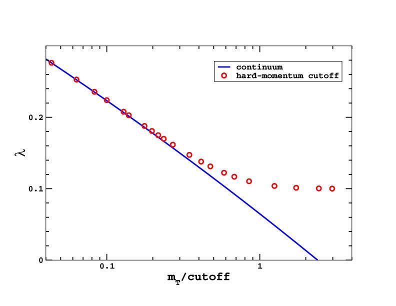
Outline of Lecture Series: Higgs Physics from the Lattice

               1. Standard Model Higgs Physics
                           •    Outlook for the Higgs Particle
                           •    Standard Model Review
                           •    Expectations from the Renormalization Group
                           •    Nonperturbative Lattice Issues?

               2. Triviality and Higgs Mass Upper Bound
                           •    Renormalization Group and Triviality in Lattice Higgs and Yukawa couplings
                           •    Higgs Upper Bound in 1-component φ4 Lattice Model
                           •    Higgs Upper Bound in O(4) Lattice Model
                           •    Strongly Interacting Higgs Sector?
                           •    Higgs Resonance on the Lattice

               3. Vacuum Instability and Higgs Mass Lower Bound
                           •    Vacuum Instability and Triviality in Top-Higgs Yukawa Models
                           •    Chiral Lattice Fermions
                           •    Top-Higgs and Top-Higgs-QCD sectors with Chiral Lattice Fermions
                           •    Higgs mass lower bound
                           •    Running couplings in 2-loop continuum Renormalization Group

Julius Kuti, University of California at San Diego   INT Summer School on ”Lattice QCD and its applications” Seattle, August 8-28, 2007, Lecture 2: Triviality and Higgs Mass Upper Bound   2/37
Standard Model Scales: Running Higgs coupling
1-loop Higgs couplings:
1-loop Feynman diagrams: Higgs boson
self-couplings
Running Higgs coupling λ(t) is defined as the
Higgs 4-point function at scale t=log µp
dλ(t)
Higgs beta function: βλ (t) = dt
Julius Kuti, University of California at San Diego INT Summer School on ”Lattice QCD and its applications” Seattle, August 8-28, 2007, Lecture 2: Triviality and Higgs Mass Upper Bound 3/37Standard Model Scales: Running gauge and Yukawa couplings
1-loop gauge couplings:
1-loop Feynman diagrams: gauge boson
couplings to fermions
Running gauge couplings g(t), g0 (t), g3 (t) can
be defined as the gauge-fermion 3-point
function at scale t=log µp
dg(t)
gauge beta functions: βg (t) = dt
1-loop Yukawa couplings:
1-loop Feynman diagrams: Higgs boson
Yukawa couplings to fermions
Running Top coupling gTop (t) is defined as
the Higgs fermion 3-point function at scale
t=log µp
dgTop (t)
Top beta function: βgTop (t) = dt
Julius Kuti, University of California at San Diego INT Summer School on ”Lattice QCD and its applications” Seattle, August 8-28, 2007, Lecture 2: Triviality and Higgs Mass Upper Bound 4/37Standard Model Scales: RG Fixed Points and Triviality
running of λ, gt , g3
I Top-Higgs sector (1-loop)
2
λ m2H
with notation R = =
g2t 4m2t
dg2t
dt = 16π2 gt
1.5 9 4
= =g32
g2t dR2 = 13 (8R2+ R − 2)
dgt
1 √
IR fixed line at R̄ = 16
1
( 65 − 1) = 0.44
H
Trivial fixed point only!
0.5
Is the Landau pole the upper bound?
Is λ(Λ) = 0 the lower bound?
00
t = gt2=g32
1 2 3 4
I Top-Higgs-QCD sector (1-loop)
Pendleton-Ross fixed point:
q √
mt = 9 g3 (µ = mt )v/ 2 ≈ 95 GeV
2
q √ √
mH = ( 689−25
72 g3 2v ≈ 53 GeV
Weak gauge couplings and 2-loop destabilize the Pendleton-Ross fixed point
“Landau pole” only in α1 at µ = 1041 GeV with all couplings running?
Julius Kuti, University of California at San Diego INT Summer School on ”Lattice QCD and its applications” Seattle, August 8-28, 2007, Lecture 2: Triviality and Higgs Mass Upper Bound 5/37Landau pole in perturbation theory: Higgs mass upper bound
The RGE in the pure Higgs sector is known to three-loop order in the MS scheme
dλ 3 39 3 7176 + 4032ζ(3) 4
β(λ) = = 2 λ2 − λ + λ .
dt 2π 32π4 (16π2 )3
The RGE exhibits an IR attractive fixed point λ=0 (perturbative “triviality”) with general
solution in one loop order
1 λ(µ)
λ(µ) = , λ(Λ) = .
1 + 3 ln Λ 1− 3
λ(µ)ln Λµ
λ(Λ) 2π2 µ 2π2
Increasing λ(µ) at fixed λ(Λ), the Landau pole is hit at 3
2π2
λ(µ)ln Λµ = 1 with the naive upper
2π2 m2H
bound λ(µ) < which is related to the upper bound on the Higgs mass λ = .
3ln Λ
µ
v2
When we try to increase λ(µ) at fixed λ(Λ) beyond the Landau pole limit, something else will
happen which will reveal the intrinsic non-removable cutoff in the theory. This will be
illustrated in the large N limit of the Higgs-Yukawa fermion model.
Julius Kuti, University of California at San Diego INT Summer School on ”Lattice QCD and its applications” Seattle, August 8-28, 2007, Lecture 2: Triviality and Higgs Mass Upper Bound 6/37Functional integral saddle point: Large NF limit of Top-Higgs model
The Lagrangian density of the continuum model after rescaling the coupling constants:
1 y 1 λ 4
L=
φ − + m2 )φ + ψ̄i γµ ∂µ ψi − √ ψ̄i ψi φ + φ , i = 1, 2, ...NF .
2 NF 24 NF
√
With rescaling of the scalar field φ → NF and integrating out the fermion fields, the partition
function is given by
Z " Z !#
1 1 4
Z= Dφ exp −NF −Tr ln(γµ ∂µ − yφ) + d4 x[ φ(− + m2 )φ + λφ ] .
2 24
The NF → ∞ limit is a saddle point for the functional integral. The solution of the saddle point
equations is equivalent to summing all Feyman diagrams with leading fermion bubbles which
are proportional to NF .
Julius Kuti, University of California at San Diego INT Summer School on ”Lattice QCD and its applications” Seattle, August 8-28, 2007, Lecture 2: Triviality and Higgs Mass Upper Bound 7/37Renormalization: Large NF limit of Top-Higgs model
I We first consider a Higgs-Yukawa model of a single real scalar field coupled to NF
massless fermions in the exact NF → ∞ limit
Julius Kuti, University of California at San Diego INT Summer School on ”Lattice QCD and its applications” Seattle, August 8-28, 2007, Lecture 2: Triviality and Higgs Mass Upper Bound 8/37Renormalization: Large NF limit of Top-Higgs model
I We first consider a Higgs-Yukawa model of a single real scalar field coupled to NF
massless fermions in the exact NF → ∞ limit
I This will allow us to demonstrate that the theory is trivial and the supposed vacuum
instability is an artifact of ignoring the necessary cutoff in the model
I Bare Lagrangian of the Higgs-Yukawa theory in Euclidean space-time is defined by
1 2 2 1 1 2
L= m φ + λ0 φ40 + ∂µ φ0 + ψ̄a0 γµ ∂µ + y0 φ0 ψa0 ,
2 0 0 24 2
I where a = 1, ..., NF sums over the degenerate fermion flavors and the subscript 0 denotes
bare quantities.
I We rewrite this as
1 2 1 1 2
L = m Zφ φ 2 + λ0 Zφ2 φ4 + Zφ ∂µ φ + Zψ ψ̄a γµ ∂µ + y0 Zφ φ ψa
p
2 0 24 2
1 2 1 1 2
= (m + δm2 )φ2 + (λ + δλ)φ4 + (1 + δzφ ) ∂µ φ
2 24 2
+(1 + δzψ )ψ̄a γµ ∂µ ψa + ψ̄a (y + δy)φψa ,
I with wavefunction renormalization factors, renormalized parameters, and counterterms
Zφ = 1 + δzφ , Zψ = 1 + δzψ ,
m20 Zφ = m2 + δm2 , λ0 Zφ2 = λ + δλ, Zψ Zφ y0 = y + δy .
p
Julius Kuti, University of California at San Diego INT Summer School on ”Lattice QCD and its applications” Seattle, August 8-28, 2007, Lecture 2: Triviality and Higgs Mass Upper Bound 8/37Renormalization: Large NF limit of Top-Higgs model
I In the limit where NF becomes large, all Feynman diagrams with Higgs loops are
suppressed relative to those with fermion loops. Hence, two of the counterterms vanish,
Renormalization conditions (1,2)
δy = 0, δzψ = 0
as there are no radiative corrections to the fermion propagator or to the Higgs-fermion
coupling.
I To maintain tree level relation m2 + 16 λv2 = 0 to all orders:
Renormalization condition (3)
Z
1 1
δm2 + δλv2 − 4NF y2 =0
6 k k2 + y2 v2
Julius Kuti, University of California at San Diego INT Summer School on ”Lattice QCD and its applications” Seattle, August 8-28, 2007, Lecture 2: Triviality and Higgs Mass Upper Bound 9/37Renormalization: Large NF limit of Top-Higgs model
I In the large NF limit, the inverse propagator of the Higgs fluctuation ϕ = φ − v is
1 1
G−1 2
ϕϕ (p ) = p2 + m2 + λv2 + p2 δzφ + δm2 + δλv2 − Σ(p2 )
2 2
y2 v2 − k.(k − p)
Z
Σ(p2 ) = −4NF y2
k (k + y v )((k − p) + y v )
2 2 2 2 2 2
We impose the condition G−1ϕϕ (p → 0) = p + mH , which separates into two
2 2 2
renormalization conditions:
Renormalization condition (4)
1
δm2 + δλv2 − Σ(p2 = 0) = 0
2
Renormalization condition (5)
dΣ(p2 )
δzφ − =0
dp2 p2 =0
Julius Kuti, University of California at San Diego INT Summer School on ”Lattice QCD and its applications” Seattle, August 8-28, 2007, Lecture 2: Triviality and Higgs Mass Upper Bound 10/37Counterterms: Large NF limit of Top-Higgs model
I Renormalization condition δm2 + 12 δλv2 − Σ(p2 = 0) = 0 maintains the tree-level relation
m2H = m2 + 21 λv2 = 13 λv2 exactly. The counterterms precisely cancel all the finite and
infinite radiative contributions.
I The Higgs mass defined as the zero-momentum piece of G−1 ϕϕ is identical to the curvature
00 (v). True physical mass given by the pole of the propagator and the renormalized
Ueff
masses mH and m can be related in perturbation theory.
I Renormalization conditions (3) and (4) yield
k2 + 2y2 v2
Z
δm2 = 4NF y2 ,
(k2 + y2 v2 )2
k
Z
1
δλ = −24NF y4 .
k (k + y v )
2 2 2 2
The closed form for δzφ is more complicated and less illuminating.
I To demonstrate triviality , we use some finite cutoff in the momentum integrals and
examine what occurs as this cutoff is removed. We will use a simple hard-momentum
cutoff |k| ≤ Λ. Exactly the same conclusions would be reached using instead
e.g. Pauli-Villars regularization.
Julius Kuti, University of California at San Diego INT Summer School on ”Lattice QCD and its applications” Seattle, August 8-28, 2007, Lecture 2: Triviality and Higgs Mass Upper Bound 11/37Counterterms: Large NF limit of Top-Higgs model
I The non-zero counterterms are
NF y2 1 2 y4 v4
" #
1 2 2
δm2 = Λ + − y v
2π2 2 2(Λ2 + y2 v2 ) 2
3NF y 4 "
y2 v2 1 1 y2 v2
!#
δλ = − 2 − − ln
π 2(Λ2 + y2 v2 ) 2 2 Λ2 + y2 v2
2 y v +Λ
2 2 2 −5Λ − 3Λ2 y2 v2
4
" ! #
NF y 1
δzφ = − 2 ln + .
2π 4 y2 v2 12(Λ2 + y2 v2 )2
I In the large NF limit, the fermion inverse propagator receives no radiative correction,
ψψ (p) = pµ γµ + yv, so we identify the fermion mass as mT = yv.
G−1
I Because both δy and δzψ vanish, we can substitutey2 = Zφ y20
−1
NF y20
Λ2 5
Zφ = 1 + − .
ln
8π2 m2T 3
For any finite bare Yukawa coupling y0 , the Higgs wavefunction renormalization factor Zφ
vanishes logarithmically as the cutoff is removed, mT /Λ → 0.
This same logarithmic behavior will appear in all of the renormalized couplings, for any
choice of bare couplings. Triviality: a finite cutoff must be kept to maintain non-zero
interactions.
Julius Kuti, University of California at San Diego INT Summer School on ”Lattice QCD and its applications” Seattle, August 8-28, 2007, Lecture 2: Triviality and Higgs Mass Upper Bound 12/37Triviality: Large NF limit of Top-Higgs model
Explicitly, the renormalized Yukawa coupling is
−1
NF y20 Λ2 5
= y20 Zφ = y20 1 +
y2 ln −
8π2 m2T 3
−1
NF Λ 2 mT
2 ln 2 ,
→ as → 0.
8π mT Λ
For the renormalized Higgs coupling, we have
m2T 1 1 m2T
3NF y4
λ = λ0 Zφ2 − δλ = λ0 Zφ2 +
− − ln
π2
2(Λ2 + m2T ) Λ2 + m2T
2 2
4
3NF y0 1 1 m2T
Zφ2 λ0 +
→ − − ln
π2 2 2 Λ2
−1
NF Λ2 mT
→ 12 2 ln 2 , as → 0.
Λ
8π mT
Julius Kuti, University of California at San Diego INT Summer School on ”Lattice QCD and its applications” Seattle, August 8-28, 2007, Lecture 2: Triviality and Higgs Mass Upper Bound 13/37Triviality: Large NF limit of Top-Higgs model
The slow logarithmic vanishing of y and λ enables a relatively large separation of cutoff and
physical scales and still maintain significant interactions. Such a theory can in some limited
sense be considered physical, if the cutoff effects are sufficiently small.
The ratio of the Higgs and fermion masses in the large NF is
m2H λv2 λ mT
= = 2 → 4, as → 0.
m2T 3y2 v2 3y Λ
Although completely unphysical, we can also consider the limit mT /Λ
1, where the cutoff is
much below the physical scale. From Equation , we see this gives
δλ = 0, δzφ = 0,
and hence Zφ → 1. In this limit, the connection between bare and renormalized parameters is
simply
λ = λ0 , y = y0 .
This result is not surprising: deep in the cutoff regime, we simply have the bare theory, with no
separation into renormalized parameters and their counterterms. This will be relevant when we
discuss the Landau pole and the vacuum instability.
Julius Kuti, University of California at San Diego INT Summer School on ”Lattice QCD and its applications” Seattle, August 8-28, 2007, Lecture 2: Triviality and Higgs Mass Upper Bound 14/37Renormalization Group flow: Large NF limit of Top-Higgs model
The physical properties of the theory, at finite cutoff Λ are fixed by the choice of a complete set
of bare parameters. Using the explicit cutoff dependence of y and λ, we can calculate the
Callan-Symanzik flow of the renormalized couplings inn the mT /Λ
1 limit
dy2 NF y20 NF y 4
βy (y, λ) = Λ = −y20 Zφ−2 =−
dΛ 4π2 4π2
dλ 1 h i
βλ (y, λ) = Λ = −8NF λy2 + 48NF y4
dΛ 16π2
This is exactly the same RG flow one would calculate in the large NF limit using
e.g. dimensional regularization, where the cutoff simply does not appear and the renormalized
couplings flow with the arbitrary renormalization scale µ. The overall signs of the β functions
would be opposite: increasing Λ corresponds to decreasing µ).
We should expect this: when the cutoff is far above the physical scales, the finite cutoff effects
are negligible and we must reproduce the unique cutoff-independent β functions.
However, as the cutoff is reduced and mT /Λ increases, this cannot continue to hold
indefinitely, as the renormalized couplings must eventually flow to the bare ones!
Julius Kuti, University of California at San Diego INT Summer School on ”Lattice QCD and its applications” Seattle, August 8-28, 2007, Lecture 2: Triviality and Higgs Mass Upper Bound 15/37Renormalization Group flow: Large NF limit of Top-Higgs model
Let us demonstrate an explicit example of the Callan-Symanzik RG flow. In the large NF limit,
mT = yv = y0 v0 . The bare vev is determined by the minimum of the bare effective potential
Z
1 1 h i
Ueff,0 = m20 φ20 + λ0 φ40 − 2NF ln 1 + y20 φ20 /k2 .
2 24 k
Using a hard-momentum cutoff, this gives
NF y20 1 2 1 2 2 y20 v20
1
m20 + λ0 v20 − Λ + y v ln = 0.
2π2 2 2 0 0 Λ2 + y20 v20
6
We express all dimensionful quantities in units of the cutoff Λ. We pick some fixed values for
λ0 and y0 . Varying the value of m20 /Λ2 changes the solution v0 /Λ of Equation and hence the
ratio mT /Λ. As we said, choosing the values of the bare parameters completely determines
everything in the theory. For example, to attain a very small value of mT /Λ requires m20 /Λ to be
precisely fine tuned! This is the origin of the so-called fine-tuning problem.
The critical surface, where v0 /Λ = 0, is the transition line
m20 NF y20
− =0,
Λ2 4π2
with all counterterms and renormalized parameters expressed in terms of λ0 , y0 , m20 and v0 .
Julius Kuti, University of California at San Diego INT Summer School on ”Lattice QCD and its applications” Seattle, August 8-28, 2007, Lecture 2: Triviality and Higgs Mass Upper Bound 16/37Renormalization Group flow: Large NF limit of Top-Higgs model
All of the counterterms and renormalized
parameters can be expressed in terms of
λ0 , y0 , m20 and v0 .
We make an arbitrary choice λ0 = 0.1,
y0 = 0.7 and vary the value of m20 /Λ2 to
explore the range 10−13 < mT /Λ < 102 .
When the cutoff is high, the exact RG flow is
exactly the same as if the cutoff had been
completely removed and follows precisely the
continuum form of Equation.
However, as the cutoff is reduced, the exact
RG flow eventually breaks away from the
continuum form and reaches a plateau at the
value of the bare coupling.
running Higgs coupling (Holland,JK)
Julius Kuti, University of California at San Diego INT Summer School on ”Lattice QCD and its applications” Seattle, August 8-28, 2007, Lecture 2: Triviality and Higgs Mass Upper Bound 17/37Renormalization Group flow: Large NF limit of Top-Higgs model
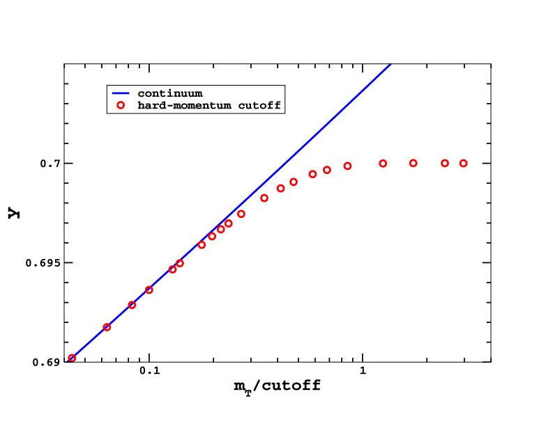
All of the counterterms and renormalized
parameters can be expressed in terms of
λ0 , y0 , m20 and v0 .
We make an arbitrary choice λ0 = 0.1,
y0 = 0.7 and vary the value of m20 /Λ2 to
explore the range 10−13 < mT /Λ < 102 .
When the cutoff is high, the exact RG flow is
exactly the same as if the cutoff had been
completely removed and follows precisely the
continuum form of Equation.
However, as the cutoff is reduced, the exact
RG flow eventually breaks away from the
continuum form and reaches a plateau at the
value of the bare coupling.
running Top coupling (Holland,JK)
Julius Kuti, University of California at San Diego INT Summer School on ”Lattice QCD and its applications” Seattle, August 8-28, 2007, Lecture 2: Triviality and Higgs Mass Upper Bound 18/37Higgs Mass Upper Bound: 1-component Higgs field
1-component lattice φ4 model is characterized by two bare parameters κ, λ with lattice action
X 4
X
S= −2κ
φ(x)φ(x + µ̂) + φ(x)2
+ λ(φ(x)2
− 1) 2
.
x µ=1
There are two phases separated by a line of critical points κ = κc (λ). For κ > κc (λ) the symmetry
is spontaneously broken and the bare field φ(x) has a non-vanishing expectation value v.
Julius Kuti, University of California at San Diego INT Summer School on ”Lattice QCD and its applications” Seattle, August 8-28, 2007, Lecture 2: Triviality and Higgs Mass Upper Bound 19/37Higgs Mass Upper Bound: 1-component Higgs field
Study the vacuum expectation value and the connected two-point function
G(x) = hφ(x)φ(0)ic = hφ(x)φ(0)i − v2 .
A renormalized mass mr and a field wave function renormalization constant Zr are defined
through the behavior of Fourier transform of G(x) for small momenta:
n o
G̃(k)−1 = Zr−1 m2r + k2 + O(k4 ) .
We also define the normalization constant associated with the canonical bare field through
Zˆr = 2κZr = 2κm2r χ .
In the framework of perturbation theory correlation functions of the multiplicatively
renormalized field
φr (x) = Zr−1/2 φ(x) ,
have at all orders finite continuum limits after mass and coupling renormalization are taken into
account. Correspondingly a renormalized vacuum expectation value is defined through
vr = vZr−1/2 .
Finally a particular renormalized coupling is defined by
gr ≡ 3m2r /v2r = 3m4r χ/v2 .
Julius Kuti, University of California at San Diego INT Summer School on ”Lattice QCD and its applications” Seattle, August 8-28, 2007, Lecture 2: Triviality and Higgs Mass Upper Bound 20/37Higgs Mass Upper Bound: 1-component Higgs field
The renormalization group equations predict that the mass and vacuum expectation value go to
zero according to
mr ≈ τ1/2 |ln(τ)|−1/6 ,
vr ≈ τ1/2 |ln(τ)|1/3 ,
for τ = κ/κc − 1 → 0, and correspondingly the renormalized coupling is predicted to go to zero
logarithmically which is the expression of triviality.
The critical behavior in the broken phase is conveniently expressed in terms of three integration
constants Ci0 , i = 1, 2, 3 appearing in the critical behaviors:
3
mr = C10 (β1 gr )17/27 e−1/β1 gr {1 + O(gr )} , β1 = ,
16π2
( )
7 gr
Zr = C20 1 − + O(g2r ) ,
36 16π2
1 0 2 −1/3
κ − κc = C m g {1 + O(gr )} .
2 3 r r
These constants were estimated by relating them to the corresponding constants Ci in the
symmetric phase. These in turn were computed by integrating the renormalization group
equations with initial data on the line κ = 0.95κc (λ) obtained from high temperature expansions.
Julius Kuti, University of California at San Diego INT Summer School on ”Lattice QCD and its applications” Seattle, August 8-28, 2007, Lecture 2: Triviality and Higgs Mass Upper Bound 21/37Higgs Mass Upper Bound: 1-component Higgs field
One massive Higgs particle
analytic results: Lüscher, Weisz
lattice simulations: JK,Lin,Shen
mR
v ≈ 3.2 at amR = 0.5
How far can we lower the cutoff?
Julius Kuti, University of California at San Diego INT Summer School on ”Lattice QCD and its applications” Seattle, August 8-28, 2007, Lecture 2: Triviality and Higgs Mass Upper Bound 22/37Higgs Mass Upper Bound: 4-component O(4) Higgs model
One massive Higgs particle +
3 Goldstone particles
analytic results: Lüscher, Weisz
lattice simulations: JK,Lin,Shen
mR
v ≈ 2.6 at amR = 0.5
How far can we lower the cutoff?
Julius Kuti, University of California at San Diego INT Summer School on ”Lattice QCD and its applications” Seattle, August 8-28, 2007, Lecture 2: Triviality and Higgs Mass Upper Bound 23/37Higgs Mass Upper Bound: 4-component O(4) Higgs model
δ measures cutoff effects in
Goldstone-Goldstone scattering
Lüscher, Weisz
Ad hoc and connected with lattice
artifacts
But threshold of new physics is in
the continuum!
What do we do when cutoff is low?
Julius Kuti, University of California at San Diego INT Summer School on ”Lattice QCD and its applications” Seattle, August 8-28, 2007, Lecture 2: Triviality and Higgs Mass Upper Bound 24/37Higgs Physics and the Lattice
Continuum Wilsonian RG
UV Completion
unknon new physics
-
Julius Kuti, University of California at San Diego INT Summer School on ”Lattice QCD and its applications” Seattle, August 8-28, 2007, Lecture 2: Triviality and Higgs Mass Upper Bound 25/37Higgs Physics and the Lattice
Continuum Wilsonian RG
UV Completion
unknon new physics
-
Below new scale M integrated UV completion
is represented by non-local Leff with all
higher dimensional operators,
1 1 λ6
φ2 φ, 4 φ3 φ, 2 φ6 , ...
M2 M M
/M ) 2 2
Propagator K(p
p2 +M 2
with analytic K thins out
UV completion with exponential damping
-
At the symmetry breaking scale v = 250 GeV
only relevant and marginal operators survive
Only 21 m2H φ2 and λφ4 terms in VHiggs (φ),
in addition to (∇φ)2 operator
Narrow definition of Standard Model: only
relevant and marginal operators at scale M
Julius Kuti, University of California at San Diego INT Summer School on ”Lattice QCD and its applications” Seattle, August 8-28, 2007, Lecture 2: Triviality and Higgs Mass Upper Bound 25/37Higgs Physics and the Lattice
Continuum Wilsonian RG Lattice Wilsonian RG
Regulate with lattice at scale Λ = π/a
UV Completion Llattice has all higher dimensional operators
unknon new physics a2 φ2 φ, a4 φ4 φ, a2 λ6 φ6 , ...
-
Below new scale M integrated UV completion
is represented by non-local Leff with all
higher dimensional operators,
1 1 λ6
φ2 φ, 4 φ3 φ, 2 φ6 , ...
M2 M M
/M ) 2 2
Propagator K(p
p2 +M 2
with analytic K thins out
UV completion with exponential damping
-
At the symmetry breaking scale v = 250 GeV At the physical Higgs scale v = 250 GeV only
only relevant and marginal operators survive relevant and marginal operators survive
Only 21 m2H φ2 and λφ4 terms in VHiggs (φ), Only 12 m2H φ2 and λφ4 terms in VHiggs (φ), in ad-
in addition to (∇φ)2 operator dition to (∇φ)2 operator
Narrow definition of Standard Model: only Choice of Llattice is irrelevant unless crossover
phenomenon is required to insert intermidate M
relevant and marginal operators at scale M scale Two-scale problem for the lattice
Julius Kuti, University of California at San Diego INT Summer School on ”Lattice QCD and its applications” Seattle, August 8-28, 2007, Lecture 2: Triviality and Higgs Mass Upper Bound 25/37Higgs Physics and the Lattice
Continuum Wilsonian RG Lattice Wilsonian RG
Regulate with lattice at scale Λ = π/a
UV Completion Llattice has all higher dimensional operators
unknon new physics a2 φ2 φ, a4 φ4 φ, a2 λ6 φ6 , ...
-
Below new scale M integrated UV completion Scale M missing?
is represented by non-local Leff with all Possible to insert intermediate continuum scale
higher dimensional operators, M with Leff to include
1 1 λ6 1 1 λ6
φ2 φ, 4 φ3 φ, 2 φ6 , ... φ2 φ, 4 φ3 φ, 2 φ6 , ...
M2 M M M2 M M
2 /M 2 ) to represent new degreese of freedom above M
Propagator K(pp2 +M 2
with analytic K thins out
or, Lee-Wick and other UV completions
UV completion with exponential damping
which exist above scale M (not effective theories!)
-
At the symmetry breaking scale v = 250 GeV At the physical Higgs scale v = 250 GeV only
only relevant and marginal operators survive relevant and marginal operators survive
Only 21 m2H φ2 and λφ4 terms in VHiggs (φ), Only 12 m2H φ2 and λφ4 terms in VHiggs (φ), in ad-
2
in addition to (∇φ) operator dition to (∇φ)2 operator
Narrow definition of Standard Model: only Choice of Llattice is irrelevant unless crossover
phenomenon is required to insert intermidate M
relevant and marginal operators at scale M scale Two-scale problem for the lattice
Julius Kuti, University of California at San Diego INT Summer School on ”Lattice QCD and its applications” Seattle, August 8-28, 2007, Lecture 2: Triviality and Higgs Mass Upper Bound 25/37Example for UV Completion: Higer derivative (Lee-Wick) Higgs sector
Jansen,JK,Liu, Phys. Lett. B309 (1993) p.119 and p.127
(Model was recently reintroduced by Grinstein, O’Connell, Wise in arXiv:0704.1845)
I Represent the Higgs doublet with four real components φa which transform in the vector
representation of O(4) and include new higher derivative terms in the kinetic part of the
O(4) Higgs Lagrangian,
1 cos(2Θ) 1
LH = ∂µ φ a ∂µ φ a − φa φa + ∂µ φa ∂µ φa − V(φa φa )
2 M2 2M 4
I The Higgs potential is V(φa φa ) = − 12 µ2 φa φa + λ(φa φa )2 .
I The higher derivative terms of the Lagrangian lead to complex conjugate ghost pairs in the
spectrum of the Hamilton operator
I Complex conjugate pairs of energy eigenvalues and the related complex pole pairs in the
propagator are parametrized by M = Me±iΘ . Choice Θ = π/4 simplifies.
I The absolute value M of the complex ghost mass M will be set on the TeV scale
I Unitary S-matrix, macroscopic causality, Lorent invariance?
λ > 0 asymptotically !
Vacuum instability ?
Julius Kuti, University of California at San Diego INT Summer School on ”Lattice QCD and its applications” Seattle, August 8-28, 2007, Lecture 2: Triviality and Higgs Mass Upper Bound 26/37Example for UV Completion: Gauged Lee-Wick extension
I Higher derivative Yang-Mills gauge Lagrangian for the SU(2)L × U(1) weak gauge fields
µ = δ ∂µ + gf
Wµ , Bµ follows similar construction with covariant derivative Dab ab abc W c ,
µ
1 1
LW = − Gaµν Gaµν − D2 Gaµν D2 Gaµν ,
4 4M 4
I LW is superrenormalizable but not finite.
I Full gauged Higgs sector is described by the Lagrangian L = LW + LB + LHiggs ,
1
LHiggs = (Dµ Φ)† Dµ Φ + (Dµ D† DΦ)† (Dµ D† DΦ) − V(Φ† Φ)
2M 4
0
I Gauge-covariant derivative is Dµ Φ = ∂µ + i 2g σ · Wµ + i g2 Bµ Φ.
I Similar fermion construction: Lfermion = iΨ6D Ψ + i
2M 4
Ψ 6 2D
D 6 2 Ψ.
6 D
SM particle content is doubled
Logarithmic divergences only
Julius Kuti, University of California at San Diego INT Summer School on ”Lattice QCD and its applications” Seattle, August 8-28, 2007, Lecture 2: Triviality and Higgs Mass Upper Bound 27/37Higher derivative β-function and RG: Lee-Wick UV Completion
Liu’s Thesis (1994)
β function:
I Higher derivative Higgs sector is finite
field theory
I Mass dependent β(t)-function
vanishes asymptotically
I Grows logarithmically in gauged
Higgs sector
running Higgs coupling:
I Running Higgs coupling λ(t) freezes
asymptotically
I The fixed line of allowed Higgs
couplings must be positive!
I Vacuum instability?
Higgs mass lower bound from λ(∞) > 0
Julius Kuti, University of California at San Diego INT Summer School on ”Lattice QCD and its applications” Seattle, August 8-28, 2007, Lecture 2: Triviality and Higgs Mass Upper Bound 28/37S-matrix, Unitarity, and Causality: Lee-Wick UV Completion
Liu,Jansen,JK
Nucl.Phys. B34 (1994) p.635
cross section phase shift
I Equivalence theorem, Goldstone
scattering
I Higgs mass upper bound relaxed
I mH =1 TeV, or higher,
but ρ-parameter and other Electroweak
precision?
I Phase shift reveals ghost, microscopic
time advancement, only π/2 jump in
phase shift
mH =1 TeV, M = 3.6 TeV
What about the ρ-parameter?
v/M=0.07, mH /M = 0.28
Julius Kuti, University of California at San Diego INT Summer School on ”Lattice QCD and its applications” Seattle, August 8-28, 2007, Lecture 2: Triviality and Higgs Mass Upper Bound 29/37The ρ-parameter
m2W Z (+)
ρ= =1+
m2Z cos2 θW Z ( 0)
cosθW is determined independently in high precision lepton processes. The 1-loop vacuum
polarization operator will shift the physical pole locations for the weak gauge bosons:
ΠH
W ΠH
Z
ρ − 1|Higgs = 2
− 2
MW,tree MZ,tree
d4 k ΣH (k2 )
Z
3
= − g02
4 k2Higgs resonance: Finite width in finite volume?
I Energy spectrum of two-particle states in a finite box with periodic boundary conditions
=⇒ elastic scattering phase shifts in infinite volume
Julius Kuti, University of California at San Diego INT Summer School on ”Lattice QCD and its applications” Seattle, August 8-28, 2007, Lecture 2: Triviality and Higgs Mass Upper Bound 31/37Higgs resonance: Finite width in finite volume?
I Energy spectrum of two-particle states in a finite box with periodic boundary conditions
=⇒ elastic scattering phase shifts in infinite volume
I Two-particle energy levels are calculable by Monte Carlo techniques =⇒ extract phase
shifts from numerical simulations on finite lattices
I Infinite bare λ limit =⇒ 4-dimensional O(4) non-linear σ-model in broken phase with
unstable Higgs particle
I Small Goldstone mass is required by the method =⇒ add external source term to the lattice
action of the 4-dimensional O(4) non-linear σ-model:
4
φαx φαx+µ̂ + J
XX X
S = −2κ φ4x
x µ=1 x
The scalar field is represented as a four component vector φαx of unit length: φαx φαx = 1
Two Goldstone bosons (“pions”) of mass mπ with zero total momentum in a cubic box of size
L3 in the elasticqregion are characterised by centre-of-mass energies W or momenta ~k defined
through W = 2 m2π + ~k 2 , k = |~k | with W and k in the ranges:
√
2mπ < W < 4mπ ⇔ 0 < k/mπ < 3
They are classified according to irreducible representations of the cubic group. Their discrete
energy spectrum Wj , j = 0, 1, 2, . . . , is related to the scattering phase shifts δl with angular
momenta l which are allowed by the cubic symmetry of the states
Julius Kuti, University of California at San Diego INT Summer School on ”Lattice QCD and its applications” Seattle, August 8-28, 2007, Lecture 2: Triviality and Higgs Mass Upper Bound 31/37Higgs resonance: Finite width in finite volume?
In the subspace of cubically invariant states only angular momenta l = 0, 4, 6, . . . contribute.
Due to the short-range interaction it seems reasonable to neglect all l , 0. Then qan energy value
Wj belongs to the two-particle spectrum, if the corresponding momentum kj = (Wj /2)2 − m2π
is a solution of !
kj L
δ0 (kj ) = −φ + jπ
2π
The continuous function φ(q) is given by
qπ3/2
tan (−φ(q)) = , φ(0) = 0
Z00 (1, q2 )
with Z00 (1, q2 ) defined by analytic continuation of
1 X 2 −s
Z00 (s, q2 ) = √ ~n − q2 .
4π ~n ∈Z3
This result holds only for 0 < q2 < 9, which is fulfilled in our simulations, and provided finite
volume polarisation effects and scaling violations are negligible
In our Monte-Carlo investigation we calculate the momenta kj corresponding to the two-particle
energy spectrum Wj for a given size L, and can then read off the scattering phaseshift δ0 (kj )
from its defining equation In order to scan the momentum dependence of the phase shift we
have to vary the spatial extent L of the lattice
Julius Kuti, University of California at San Diego INT Summer School on ”Lattice QCD and its applications” Seattle, August 8-28, 2007, Lecture 2: Triviality and Higgs Mass Upper Bound 32/37Higgs resonance: Finite width in finite volume?
I The two-particle states in our model are also classified according to the remaining
O(3)-symmetry: They have “isospin” 0, 1, 2. Since we expect the σ-resonance to be in the
isospin-0 channel, we restrict ourselves to that case.
I Operator O0 (t) = Φ̃~4 = L−3 ~x Φ~4x ,t for σ-field at zero momentum is included
P
0 ,t
I Two-particle
D correlation matrix
function
E
Cij (t) = Oi (t) − Oi (t + 1) Oj (0) i, j = 0, 1, 2, . . .
I Eigenvalues decaying as exp(−Wi t)
I The set of states is truncated at finite i = r to keep Wr below inelastic threshold
J m =2m =3m =4m
I Lines of constant ratios mσ /mπ
and mπ L (dotted line)
I Reflection multi-cluster algorithm for finite
external source J
I Set of 3 κ, J configurations with middle point
κ = 0.315, J = 0.01 tuned to keep σ-mass in
elastic region
I Cylindrical lattices L3 · T up to sizes of 243 · 32,
323 · 40
c
Figure 3: Lines of constant mass ratios m =m and m L in the -J plane derived with the
help of
Julius theUniversity
Kuti, scaling laws of ref. at[22].
of California San The
Diegosolid
lineINT
represents the ratio
Summer School m =mQCD
on ”Lattice = 3.
andOur choice Seattle, August 8-28, 2007, Lecture 2: Triviality and Higgs Mass Upper Bound
its applications” 33/37Higgs resonance: Finite width in finite volume?
I The pion mass mπ can be measured by a fit to the inverse propagator in four-dimensional
momentum space:
aa (p, −p) = Zπ {mπ + p̂ }, a = 1, 2, 3
G−1 −1 2 2
I For perturbation theory checks we also want mσ and λR ,
m2σ − m2π
λR = 3Zπ
Σ2
where Σ is the infinite volume σ field expectation value
I Two-parameter fit to the inverse σ and π propagators in momentum space
I 323 · 40 lattice at κ = 0.315, J = 0.01
[ G44 (p; ?p)]?1
and
I The negative intercept and slope of the
inverse Goldstone propagator G−1
aa (p, −p)
[Gaa(p; ?p)]?1 determine the propagator mass mπ
I The negative intercept and slope of the
inverse σ propagator G−1
44 (p, −p)
determine the propagator mass mσ for
the Higgs particle
pb2
Julius Kuti,Figure : The upper (lower) curve INT
University5of California at San Diego shows a two-parameter
Summer t to and
School on ”Lattice QCD theitsinverse ()Seattle,
applications” propagator
August 8-28, 2007, Lecture 2: Triviality and Higgs Mass Upper Bound 34/37Higgs resonance: Two-particle states
W
m I Comparison of simulation results
(crosses) with perturbative prediction in
isospin 0 channel at κ = 0.315, J = 0.01
I Solid lines depict perturbative prediction
(dashed lines perturbative estimates
based on propagator masses)
I Dotted lines represent free pion pairs
I The location of the resonance energy mσ
is indicated by dotted horizontal line at
W ≈ 3mπ
m L
Figure 8: Comparison of the Monte Carlo results (crosses) with the perturbatively predicted
two-particle energy spectrum in the isospin-0 channel for the simulation point ( = 0:315,
J = 0:01). The data are in excellent agreement with the perturbative predictions (solid lines)
based on the results of table 11. Dotted lines refer to the free energy spectrum, while the
dashed lines show the perturbative spectrum based on the estimates of table 4. The location
of the resonance energy m is symbolized by the dotted horizontal line at W 3m . { Errors
are smaller than the symbols.
Julius Kuti, University of California at San Diego INT Summer School on ”Lattice QCD and its applications” Seattle, August 8-28, 2007, Lecture 2: Triviality and Higgs Mass Upper Bound 35/37Higgs resonance: Phase shift in perturbation theory
1. We will use the linear model for the phase shift calculation
• S[φ; j, m2 ] = d4 x 12 ∂µ φα ∂µ φα + − 12 m2 φα φα + 4!λ (φα φα )2 − jφN
R h i
• with α = 1, ..., N and N = 4 in our case.
• The mass parameter m2 is negative in broken phase
2. Pions have “isospin” index a=1,...N-1 (single pion state isospin is I=1 for N=4)
• Two-particle state decomposes into I=0,1,2 irreducible representations
∞
• Partial wave decomposition T I = 16πW (2l + 1)Pl (cosϑ)tlI
P
k
l=0
• Bose symmetry requires tlI = 0 if I+l is odd
I
2iδ
• tlI = 2i1 e l − 1 with real phase shifts δIl in elastic region 2mπ < W < 4mπ
3. Leading perturbative result:
m2 − m2π
!
N−1 k
δ00 = λR 1 − σ2 + δ20
48π W mσ − W
λR m2σ − m2π m2 4k2 + m2σ λR m2σ − m2π
! !
δ20 = 1 + σ2 ln 2
−
96π kW 2k mσ 48π kW
Julius Kuti, University of California at San Diego INT Summer School on ”Lattice QCD and its applications” Seattle, August 8-28, 2007, Lecture 2: Triviality and Higgs Mass Upper Bound 36/37Higgs resonance: Phase shift
Göckeler et al.
00
amσ = 0.72
mσ = 3.07 mπ
Γσ = 0.18 mσ
k=m
Figure 15:Agreement
Comparison of the
witht with respect to the perturbative
perturbation theory ansatz (3.6) (solid curve)
and the perturbative prediction based on the estimates m
~ and g~R of table 4 (dashed curve)
in the isospin-0 channel for ( =0:315, J =0:01).
Julius Kuti, University of California at San Diego INT Summer School on ”Lattice QCD and its applications” Seattle, August 8-28, 2007, Lecture 2: Triviality and Higgs Mass Upper Bound 37/37You can also read