Long-Term Care Insurance: Knowledge Barriers, Risk Perception and Adverse Selection - DOCUMENT DE TRAVAIL / WORKING PAPER - UQAM
←
→
Page content transcription
If your browser does not render page correctly, please read the page content below
DOCUMENT DE TRAVAIL / WORKING PAPER
              No. 2018-10

Long-Term Care Insurance: Knowledge
Barriers, Risk Perception and Adverse
               Selection

Martin Boyer, Philippe De Donder, Claude
Fluet, Marie-Louise Leroux et Pierre-Carl
                Michaud
              Janvier 2018
Long-Term Care Insurance: Knowledge Barriers,
Risk Perception and Adverse Selection
Martin Boyer, HEC Montréal, Canada
Philippe De Donder, Université du Québec à Montréal, Canada
Claude Fluet, Université Laval, Canada
Marie-Louise Leroux, Université du Québec à Montréal, Canada
Pierre-Carl Michaud, HEC Montréal, Canada; et NBER
Document de travail No. 2018-10
Janvier 2018
Département des Sciences Économiques
Université du Québec à Montréal
Case postale 8888,
Succ. Centre-Ville
Montréal, (Québec), H3C 3P8, Canada
Courriel : brisson.lorraine@uqam.ca
Site web : http://economie.esg.uqam.ca
Les documents de travail contiennent souvent des travaux préliminaires ou partiels et
sont circulés pour encourager et stimuler les discussions. Toute citation et référence à
ces documents devrait tenir compte de leur caractère provisoire. Les opinions
exprimées dans les documents de travail sont ceux de leurs auteurs et ne reflètent pas
nécessairement ceux du département des sciences économiques ou de l'ESG.
Copyright (2018): Martin Boyer, Philippe De Donder, Claude Fluet, Marie-Louise
Leroux et Pierre-Carl Michaud. De courts extraits de texte peuvent être cités et
reproduits sans permission explicite à condition que la source soit référencée de
manière appropriée.Long-Term Care Insurance: Knowledge Barriers, Risk
Perception and Adverse Selection ∗
Martin Boyer Philippe De Donder Claude Fluet
HEC Montréal ESG UQAM Université Laval
Marie-Louise Leroux Pierre-Carl Michaud
ESG UQAM HEC Montréal and NBER
December 2017
Abstract
We conduct a stated-choice experiment where respondents are asked to rate various
insurance products aimed to protect against financial risks associated with long-term
care needs. Using exogenous variation in prices from the survey design, and objective
risks computed from a dynamic microsimulation model, these stated-choice probabilities
are used to predict market equilibrium for long-term care insurance using the framework
developed by Einav et al. (2010). We investigate in turn causes for the low observed
take-up of long-term care insurance in Canada despite substantial residual out-of-pocket
financial risk. We first find that awareness and knowledge of the product is low in the
population: 44% of respondents who do not have long-term care insurance were never
o↵ered this type of insurance while overall 31% report no knowledge of the product. We
then identify three main causes for the lack of long-term care insurance: asymmetric
information, lack of awareness of the insurance products, and misperceptions of risks.
We measure the welfare losses associated to these three causes, and obtain much higher
welfare losses for lack of awareness (corresponding to 49% of the equilibrium consumer
surplus estimated with our data for the baseline contract) than for misperceptions (28%)
and especially for adverse selection (1%).
Keywords: Long-term care insurance, adverse selection, stated-preference, health,
insurance
∗
We acknowledge financial support from the Social Science and Humanities Research Council (435-2016-
1109). We wish to thank Pierre-André Chiappori, Georges Dionne, Andreas Richter, Christopher Tonetti
for helpful comments and suggestions. We thank seminar participants at the Financing Longevity Con-
ference at Stanford, KU Leuven, HEC Montreal, and the 2017 American Risk and Insurance Meetings for
their comments and suggestions. We also thank Sébastien Box-Couillard and Francois Laliberté-Auger for
excellent research assistance and David Boisclair for help with the design of the questionnaire.
11 Introduction
Because of rapid population aging, financing and providing long-term care (LTC here-
after) to older people is an important and growing problem in developed countries.1 In
OECD countries, the population of 80 years old and more is expected to grow from 4%
of the total population in 2010 to 10% by 2050 (OECD, 2011). Estimates of the proba-
bility that someone approaching retirement will use a nursing home at some point in his
life ranges from 35 to 50% in the U.S. (Brown and Finkelstein, 2009; Hurd et al., 2017).
For instance, in Québec, the out-of-pocket cost of a public nursing home (CHSLD) is
around 20,000$ a year and on average, people stay 5 years in these facilities. For peo-
ple with low savings, this can represent important amounts. Moreover, public nursing
homes provide minimum basic services so that an individual who would like to have a
“service of higher quality” would have to resort to a private nursing home whose cost
varies between 40,000$ and 60,000$ a year.2 Finally, the waiting time for accessing the
public service is around 10 months so that in the meantime, agents would have to find
alternative (private) solutions. Hence, LTC risk is associated with potentially important
financial risks for households despite subsidies from the government. Yet, few insure
privately against such risk (Pestieau and Ponthiere, 2011). In Canada, the share of total
LTC spending covered by private insurance was around 0.5% in 2010 while for OECD
countries, it was less than 2% (OECD, 2011). In Quebec, the association representing
insurers (ACCAP) reported to us that the a take-up rate for long-term care insurance
policies was around 1.7% in 2015.3 This is the so-called Long Term Care Insurance
(LTCI hereafter) Puzzle.
Many factors, both on the demand and on the supply sides can explain the lack
of a market for LTCI.4 On the supply side, it is often argued that LTCI is expensive
1
Long term care is defined as the care for people needing daily living support over a prolonged period of
time. Support can be provided with activities of daily living (such as bathing, dressing, eating, getting in
and out of bed, toiletting and continence) or instrumental activities of daily living (which include preparing
meals, cleaning, doing the laundry, taking medication, getting to places beyond walking distance, shopping,
managing money a↵airs, and using the telephone and nowadays the Internet). The loss of autonomy is most
often associated with old age and should be clearly distinguished from illness, disability and handicap.
2
Québec and Ontario provide dependents with income-related reduced fees as well as with tax-credit for
formal care in the case of Québec.
3
In the U.S., only about 10.8 percent of those 60 years and older held such a policy in 2009 (Brown and
Finkelstein, 2009).
4
See the surveys on long term care by Brown and Finkelstein (2011) and Cremer et al. (2009).
2because of important loading factors in the private provision of such insurance (Brown
and Finkelstein, 2009). Most of the evidence on this comes from the United States.
One reason could be that important asymmetric information problems exists (both
moral hazard and adverse selection). These may induce insurers to restrict coverage
and charge higher premiums (Sloan and Norton, 1997). For example, Finkelstein and
McGarry (2006) find that multiple sources of asymmetric information exist in that
market. Another reason may be the cost of getting access to public funds in the public
sector (rationing of access). This can be potentially important in some countries. For
example, Canada has substantial waiting times for public care homes (on average close
to 10 months in the province of Quebec).
On the demand side, the importance of family support, either formal or informal,
may explain the lack of LTCI. Formal help can be defined as monetary transfers while
informal help refers to help in time. Empirical evidence shows that most informal
transfers are provided by the family while formal help mostly results from private or
public insurance. Family carers are primarily spouses, adult daughters, and daughters-
in-law, as mentioned in the OECD (2011) report. Many studies have documented the
importance of family help and there is evidence of substitutability between informal
and formal help (Bonsang, 2009). Yet, insurance products in Canada are conditionned
on care needs rather than reimbursements which may yield higher demand for LTCI
as an e↵ective way of insuring the family rather than the individual being cared for
(say for earnings loss due to caring). Pauly (1990) and Brown and Finkelstein (2008)
also show that social insurance (in particular Medicaid) crowds out the demand for
private insurance. This is potentially important in Canada as public subsidies in the
form of lower co-pays for nursing homes and tax credits for formal care are means-
tested. Another substitute for insurance may be home ownership since those holding net
home equity may sell their property when moving to a nursing home (Davido↵, 2009).
Regarding preferences, Lockwood (2014) shows that bequest motives by reducing the
opportunity cost of saving increase saving and decrease purchases of LTCI.5 But the
e↵ect of bequests is ambiguous as those with such a motive may also want to purchase
insurance to guard against the risk of not leaving anything behind for their heirs due
to LTC costs.
5
See also Ameriks et al. (2011) about the importance of bequest motives for late-in-life decisions to save.
3Another reason for the lack of LTCI is related to misperception of risks. Zhou-
Richter et al. (2010) finds evidence that these biases are important to explain low
demand. Related to this issue, Finkelstein and McGarry (2006) compare the subjective
probability of entering a nursing home within 5 years for respondents aged on average
78 to the actual decisions of the same respondents after 5 years. They find that most
respondents do not estimate correctly their true probability of needing such a form of
LTC. Tennyson and Yang (2014) highlight the role of one’s experience with LTC as a
contributing factor to the awareness of the risk of LTC costs, or the lack thereof. Hence,
risk perceptions may be an important driver of low demand. Generally, lack of financial
knowledge in general, and more specifically the lack of knowledge about LTC costs and
institutional details in particular may play an important role in the decision to purchase
such insurance. Individuals often fail to evaluate correctly the size of LTC costs which
they may incur late in life and they may not be aware of eligibility rules for care,
means-testing, etc. There is a large body of empirical studies on the lack of knowledge
of basic financial concepts (Lusardi and Mitchell, 2014; Boisclair et al., 2015). These
may in turn have important consequences for saving decisions and retirement planning
(Lusardi et al., 2017). There is however not much evidence on whether agents have a
good knowledge of the true costs associated with dependency and an understanding of
the institutional setting.
The objective of this paper is to analyze which of the above reasons explain low
take-up rates, and whether these are related to factors on the demand side, on the
supply side or both. To do so, we partnered with Asking Canadians, a Canadian
online panel survey organization to field a survey on LTCI, in the fall of 2016. We
selected randomly 2000 panel members age 50 to 70 in the two most populous provinces
of Canada, Ontario and Quebec. We then matched each respondent with a health
microsimulation model capable of estimating personalized lifetime exposure to disability,
nursing home and formal care (Boisclair et al., 2016). This allows to estimate actual risk
faced by households and potentially covered by insurers and compare those with risk
perceptions we elicit in the survey. We also survey respondents about their knowledge
of LTC and institutional details and preferences for care which have been shown to
be correlated with demand for LTCI (Brown et al., 2012). We then build a stated-
4preferences experiment to study demand for LTCI.6 . The second part of our survey
consists of an experiment where we presented each respondent with the prospect of
purchasing a LTCI product. These scenarios di↵er in terms of the benefit paid in case
of dependency, the premium paid and the provision of an embedded term life insurance
contract if the respondent dies prior to age 85. From survey responses and experimental
variation in contract characteristics, we can infer the participants’ demand for LTCI
and find whether there is adverse or advantageous selection in this insurance market.
We build on the methodology developed by Einav et al. (2010) which use revealed
preferences to estimate the demand and supply curves of employer-provided health
insurance using individual-level data from a multinational producer of aluminium and
related products, Alcoa Inc. The combination of estimated demand and supply curves
enables to evaluate the welfare losses associated with asymmetric information (whether
it is adverse or advantageous selection). We extend this approach to stated-preference
data using experimental variation in prices.
Our results confirm the existence of under-insurance for LTC. Focusing on the base-
line contract o↵ering a 2000 CAD LTC monthly benefit without any life insurance, our
model predicts that the optimal proportion of agents buying LTC should be around 25%
while the equilibrium take-up rate is much lower, at 12%. Adverse selection explains
only a very tiny fraction of this gap (in the absence of adverse selection, the equilibrium
take-up rate would increase by a mere 1%), and consequently generates a very small
welfare cost, of the order of 2$ per year per person. The largest part of the take-up gap
is rather explained by the lack of awareness of LTCI products, with a much smaller role
for misperceptions regarding survival and dependence probabilities as well as LTC insti-
tutions and insurance products. We evaluate the welfare cost of this lack of awareness
at around 100$ per year per person, while it is around 57$ for misperceptions.
Few papers combine stated-preference and revealed preference data to study this
market. One exception is Ameriks et al. (2016). They use strategic survey questions
along with balance sheet data from the Vanguard Research Initiative (VRI) to estimate
preferences, within a well-defined life-cycle model, to explain the low demand for LTCI
products.7 They find that 60% of the panel members should buy LTCI according to
6
See J. Louviere (2000) on the merits and disadvantages of stated-choice experiments
7
Ameriks et al. (2015) claim that although the Vanguard Research Initiative sample “explicitly targets
5their model. In comparison, only 22% actually do buy LTCI in the panel. This gap
can be explained by a lack of interest on the demand side as well as poor insurance
product features on the supply side. In our framework, we elicit directly preferences of
respondents which allows to compute the demand curve using experimental variation
in prices without making any assumption regarding the choice problem respondents
actually solve. We also consider the supply and demand side jointly, which allows to in-
vestigate selection and equilibrium in that market. Another related paper is Dardanoni
and Li Donni (2016) who use a framework similar to ours but in a revealed preference
context. Their approach rests on evaluating welfare loss from mixture type models us-
ing external estimates of the price elasticity of demand for LTCI. They estimate large
welfare loss from unpriced heterogeneity and use large estimates of the price elasticity
of demand (-3.5 and -2). In our framework, we can estimate this elasticity directly from
the stated-preference experiment.
The paper is organized as follows. In section 2, we present the survey and the
questionnaire we used. In section 3, we present descriptive evidence from the survey.
We present an equilibrium model for LTCI products which can be applied to stated-
preference data from our survey in section 4. We present results in section 5. Finally,
section 6 concludes.
2 The Survey
2.1 Survey
Partnering with Asking Canadians, a Canadian online panel survey organization, we
conducted a survey on LTCI in late autumn 2016. We randomly selected 2000 panel
members aged 50 to 70 residing in the two largest and most populous provinces of
Canada, Ontario and Quebec. Participants are rewarded for their participation (with
loyalty rewards from major retailers). Despite those e↵orts, some groups are slightly
underrepresented, in particular low-educated and income groups. We stratified by age,
gender, province and education groups (three levels) and used the Canadian Labor Force
Survey of 2014 (the last year available) to re-weigh the data. The e↵ect of weighing was
the half of older Americans with non-trivial financial assets”, similar results would be obtained with an
appropriately conditioned sample of the HRS.
6minimal on our analysis. For example, the median household income we estimate in
the survey is 65,000$ for the province of Quebec, while the equivalent number from the
Social Policy Simulation Database (SPSD) for 2016 is 69,000$.8 The 25th percentile
of household income in the SPSD is 41110$ for Quebec while we estimate it to be
38,000$ in our survey. Hence, once reweighed, our survey appears representative of the
population age 50-70 in Quebec and Ontario.
A copy of the questionnaire (in text format) is found in Appendix A. It had 4 major
parts.9 The first three parts asked respondents about socio-economic characteristics,
reasons for having purchased (or not) LTCI, risk perceptions and, their preferences re-
garding the type of LTC they would prefer to receive. For some of these questions,
we used a formulation taken from Brown et al. (2012). For questions where we ex-
pected a significant fraction of missing information, such as savings and income, we
used unfolding brackets. We then used multiple imputation to impute missing values
with information from the bracketing, conditional on basic socio-demographic covariates
(age, gender).
The fourth and last part of the survey consisted of a stated-preference experiment.
We presented each respondent with the prospect of purchasing a LTCI product. These
scenarios di↵er in the benefit paid under LTCI, the premium and a term life insurance
if the respondent dies prior to age 85. The introductory text is reproduced below (the
equivalent existed in French for Quebec residents who are mostly French speakers).
We are going to show you some simple insurance policies and ask you to rate those.
You can assume that if you were to have two or more limitations in activities of daily
living, the insurance company o↵ering you this product would pay the benefits no matter
what the circumstances. Once you receive benefits, you do not pay any premiums.
Each product has three attributes: a) a monthly premium you have to pay; b) a
monthly benefit if you have 2 or more limitations in activities of daily living, starting
3 months after your limitations have been verified; and c) a payout to your survivors if
you die before age 85. Assume that if you are healthy and you stop paying premiums
for 3 consecutive months, the contract is cancelled and you lose coverage. The premium
cannot increase once you have purchased the product. Finally, the benefits are adjusted
for inflation (indexed).
We presented scenarios using the following representation:
8
Throughout the paper, the sign $ always refers to Canadian dollars.
9
Asking Canadians validates completed questionnaires based on a number of indicators, such as the time
of completion, and drops respondents for whom it appears that answers may be questionnable.
7While healthy Once you have at least 2 ADL When you die
You pay ⇡ You receive bltc Your survivors receive blif e
We use a simple LTCI contract on purpose. In order to avoid uncertainty about
the future premiums we explicitly mention that premiums could not increase once the
contract is signed. This means of course that in real terms the premiums are decreasing.
We also insisted on the possibility of lapse-risk in the sense that respondents were made
aware that if a payment was not made for some time, it would lead to the termination
of the contract. We mentioned that there is no risk regarding payment of benefits.
This meant that if the respondent had 2 or more ADL impairments, then the insurance
company would for sure pay the benefits that were contracted upon. We also insisted
that the product is o↵ered by a trusted insurance company. We explicitly wanted
respondents to dismiss the risks associated with nitpicky insurers (see Bourgeon and
Picard (2014)) and the insurers credit risk; in other words, we wanted to avoid having
them think of payment risk. Finally, LTCI benefits are indexed to inflation. Apart
from wanting to o↵er a situation that is closer to what occurs in reality where the LTCI
protection o↵ered in LTCI products is more often than not indexed to inflation, we also
wanted respondents to know that the amount of services they would receive in LTC is
independent of time when they become disabled.
We presented five of those scenarios to each respondent. Each time we asked re-
spondents for the likelihood with which he or she would purchase this product if it were
o↵ered by a trusted insurance company. Possible answers ranged from 0%, meaning
there was no chance whatsoever that the respondent would purchase the LTCI product,
and 100%, meaning that the respondent would certainly purchase that product. We
consider jointly LTCI and term life insurance contracts because of the potential desir-
ability of having some life insurance protection in case one dies early, prior to facing
significant disability risk.10 This bundling may be particularly interesting for respon-
dents that have some sort of bequest motive. The reason we asked for probabilities
is that they convey considerably more information than a yes or no answer and allow
to account for the fact that scenarios are incomplete (Manski, 1999). One advantage
of asking for the probability with which one would purchase a contract is that we can
10
Note however that, to the best of our knowledge, insurance products bundling LTCs and life insurance
benefits do not exist in Canada at the moment.
8use these probabilities directly in our analysis without having to make any assumptions
about the functional form that leads to a yes/no answer.
Note that waiting to purchase LTC insurance has no significant option value. On
the opposite, waiting runs the risk of sizeable increases in the insurance premium as
agents grow older. Also, there is little reclassification risk (the premium is fixed for the
duration of the contract and the lump-sum payment is made conditional on su↵ering
at least two ADL, irrespective of the severity of dependence).
Each scenario is constructed in the following way. For each respondent, a monthly
LTCI benefit bltc is first randomly picked from the distribution [2000, 1/3; 3000, 1/3; 4000, 1/3].
We also pick randomly a benefit for the life insurance component of scenario, blif e from
the distribution [0, 3/5; 10000, 1/5, 25000, 1/5]. In Canada, most insurers only use infor-
mation on age and gender to price this type of insurance. Some insurers will underwrite
insurance on the basis of pre-existing medical conditions but premiums are not a func-
tion of health status. In our research design, we will therefore concentrate on o↵ering
premiums which will consist of an age-gender actuarial premium, computed from a
microsimulation model, and a price adjustment factor which will be randomized but
centred on 1. Hence, the average premium o↵ered to respondents of a certain age
and gender group will be equal to the actuarial premium we will compute from our
microsimulation approach. Hence, we first use the health microsimulation model COM-
PAS, which we describe below, to compute by age and gender the actuarial premium
associated to these benefits, assuming a 3% discount rate. These premiums can be
compared to those observed in the market. We obtained from CAA-Quebec (which is
the Quebec equivalent of the AAA in the United States) premium data corresponding
to similar levels of coverage to those presented to respondents. In Table 1, we report
average estimates in the sample. These premiums are close to those observed in the
market, although our model estimates are higher than market premiums for men in
general, and for women at younger ages. They are, however, lower for women at older
ages.
We denote by ⇡h the actuarial premium for each class of risk (by gender and age),
h. Finally, we create exogenous variation in premiums by drawing a factor ⌧ from the
distribution
9⌧ = [0.6, 1/5; 0.8, 1/5; 1.0, 1/5; 1.2, 1/5; 1.4, 1/5].
The premium is given by ⇡ = ⌧ ⇡h . Hence a scenario consists of a triple (⇡, bltc , blif e ).
2.2 COMPAS
There is no detailed projection of disability risk in Canada that would allow us to
construct personalized risk estimates for respondents in our survey. We use the mi-
crosimulation model COMPAS that was developed to project the long-term evolution
of health and health care use in Canada (Boisclair et al., 2016).11 The structure of the
model follows from other models such as the Future Elderly Model (Goldman et al.,
2005). Each individual in the model has many characteristics :
• Socio-demographic characteristics: age, sex, immigration status, education level,
income bracket
• Diseases: diabetes, high blood pressure, heart diseases, stroke, cancer, lung dis-
eases, dementia
• risk factors: smoking, obesity
• Disability: limitations in ADLs and Instrumental ADLs (IADL)
• Long-term care: formal home care, nursing home
Based on these characteristics, the core of the model consists of a Markovian transi-
tion model of diseases, risk factors, disability and long-term care characteristics. These
transitions are based on a set of transition models which were estimated using the
National Population Health Survey (1994-2010). The transition model has been satis-
factorily tested by simulating on original 1994 data the trajectories of respondents in
the NPHS until 2010 and comparing distribution of outcomes. The model delivers sim-
ulated life-trajectories conditional on a set of initial conditions. Given the large number
of variables, one cannot construct at transition matrix across all these states. Instead,
each respondent can be simulated a large number of times and an individualized set
11
A detailed description of the model can be found here
10of disability and mortality risks can be computed by averaging over these simulations.
When designing the questionnaire for our survey, we deliberately asked questions we
could then feed directly into the health transition matrix of COMPAS. In particular, we
asked respondents for their education level, their health conditions (same as in COM-
PAS) and smoking habits. Nevertheless, data limitations are likely to impact some of
the calculations we make. COMPAS uses NPHS data which records the location of
respondents at the time of the survey but no location is available when the respondent
has been found to have died. Since nursing home stays tend to occur more frequently
at the end of life, this could impact our estimates. Hurd et al. (2017) find that shorter
stays, in particular those near the end of life are missed by core interviews in the Health
and Retirement Study. Although short stays may be missed, they may matter more for
policyholders than for insurers, as these stays are typically shorter than the deductible
threshold of LTCI policies (3-5 months). In particular, it may be that we underestimate
the individual risks while respondents have correct expectations about such risks.
Hence, we are able to construct a distribution of individualized disability and mor-
tality risks (as a function of a large number of characteristics). Since insurers do not
use these characteristics to price such insurance products, we will be able to use these
unused pricing characteristics to test for asymetric information and quantity its e↵ect
on take-up of such insurance.
3 Descriptive Evidence
3.1 Take-Up, Knowledge and Awareness of LTCI
Table 2 reports the number of people with (the rightmost column) and without (the
leftmost column) long term care insurance. We find that the take-up rate of LTCI is low,
at 11.8%, at a similar level as that found in the U.S.12 We also report the respondents’
12
This number is significantly larger than what has been previously reported, for example in Quebec. The
association representing insurers (ACCAP) reported to us that long-term care insurance policies in e↵ect
covered 39,000 persons in 2015. This would imply a take-up rate of 1.7%. It does not appear that our survey is
systematically biased in terms of socio-economic status composition to explain this di↵erence. Furthermore,
we use a similar question to that used in the U.S. and take-up from surveys tend to match estimates from
administrative data there. For life insurance, the Canadian Life and Health Insurance Association reports
22 million covered in Canada which translates into 84% coverage. Our estimate from survey for those 50 to
70 is also in that range (77%). Hence, it is unclear why our numbers for LTCI are so di↵erent.
11level of knowledge about LTCI products. Among those who did not purchase LTCI,
39.9% reported having no knowledge about the product, and 8.2% reported not knowing
what the product was. Others judged that such policies were too expensive (19%) or
unnecessary.
Among the respondents who were covered by LTCI, close to two-thirds (65%) knew
little about that type of products whereas 5.7% said they knew nothing at all. The main
reason for having purchased an LTCI policy is that they were o↵ered one through one
channel or another: only 9.6% of respondents having an LTCI policy declared having
actively searched for such a protection while 53% were o↵ered the product, suggesting
that the main channel for obtaining LTCI is likely to be through a financial advisor or
direct marketing.
The monthly premium paid was 125$ on average (all dollars values are in Cana-
dian dollars, of course; at the time of the survey, one Canadian dollar was worth the
equivalent of 0.75 US dollar) for monthly benefits of the order of 2415$ in case of loss
of autonomy. Finally, 75% of LTCI purchasers had some sort of life insurance policy
(whether term life or other), whereas 22.2% did not have one. Hence, life insurance is
much more widespread than LTCI insurance. To summarize, take-up is low but aware-
ness and knowledge of the product is also very low and likely a major driver of low
demand.
3.2 Risks and Perception
From the microsimulation model, we can compute mortality and disability risk for each
respondent based on health and socio-demographic characteristics at the time of the
survey. For each respondent, we need a set of probabilities of having limitations in
activities of daily living at future ages (from the current age of respondent i to age 110)
and similarly for survival probabilities. The microsimulation model yields simulated life
trajectories for each of the respondents. We can estimate a set of simulated probabilities
by feeding each respondent 1000 times into the simulator. We use as inputs gender, age,
education, smoking status and a set of health variables asked in the survey and used
in COMPAS (whether the respondent has had heart disease, diabetes, hypertension,
cancer, stroke and mental health problems). In Figure 1, we report the mortality risk
12for various age groups at the time of the survey. We first compute the expected number
of years of life remaining using individual level survival risk. We then order respondents,
for each age group, by percentile of the distribution of remaining life expectancy. We
report the average mortality risk within each age group and quartile. We see substantial
variations in mortality risk at all ages, which predictably becomes more pronounced at
older ages. To give an idea of the magnitudes, an individual respondent in the bottom
quartile of age bracket 50-54 has a mortality rate at age 85 that is 2.3 times higher
than an individual in the top quartile of the same age bracket. This translates into a
remaining life expectancy of 28.21 years in the bottom quartile and 38.3 years in the
top quartile. Hence, mortality risk modelling using survey respondent characteristics
yields substantial heterogeneity in survival risk.
We conduct a similar exercise for disability risk. In Figure 2, we report estimates for
disability risk conditional on having survived to a given age for each age group. We also
see substantial heterogeneity in risk by age. A respondent aged 90 faces a probability of
being disabled, and thus needing care, of the order of 20% to 30%. Given these risks, we
can estimate the lifetime risk of ever being disabled and that of ever entering a nursing
home for at least 1 year. We present these estimates from COMPAS in Figure 3. On
average respondents face a probability of being disabled of 56.1% but this risk is quite
heterogeneous in the population. Because nursing home stays are expensive, we also
compute the lifetime risk of entering a nursing home. On average respondents face a
risk of 26.2%. Again this risk is very heterogeneous in the population.
To get an idea of the financial exposure due to future LTC expenditures, we estimate
the net present value of the expenditures associated with formal care and nursing homes
for all respondents. To do this, we need estimates of the cost of a year in a nursing home.
These costs vary. The annual cost for Quebec public nursing homes is $43,000 (Boisclair
et al., 2016). We use this cost in both Quebec and Ontario for illustrative purposes. Of
course, respondents never pay the full cost. So we also compute the cost using the user
contribution currently set by the Quebec and Ontarian government at roughly $2000
per month, which amounts to $24,000 per year, out-of-pocket. For formal care, we use
an estimate of $25 per hour of formal care and the number of hours of formal care
predicted from the microsimulation model. Since the Quebec government o↵ers a tax
credit of roughly 33% of expenditures, we also compute an out-of-pocket cost measure
13for formal care expenditures. There is no such credit in Ontario. We then combine
these cost estimates with the probabilities presented earlier to estimate net present
value measures of these costs (assuming a 3% real discount rate and no excess inflation
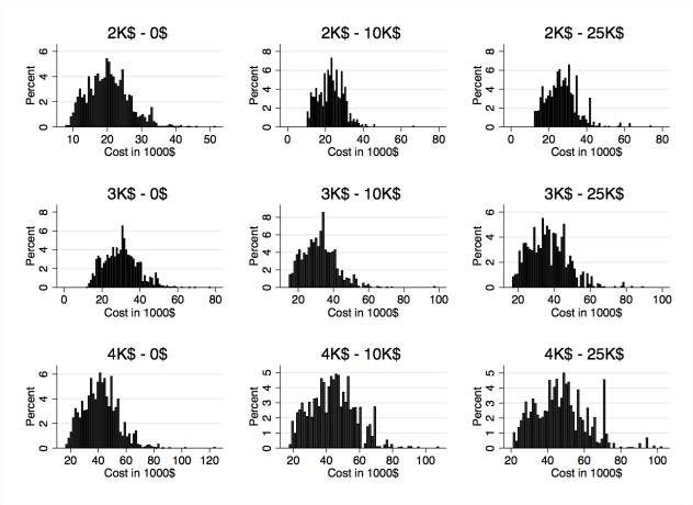
in LTC costs). These estimates are shown in Figure 4. If there was no insurance from
the government nor the private sector, on average, respondents would face an expected
LTC cost of $30,788. There is considerable heterogeneity in that risk. More than
10% of respondents face a net present value of expenditures larger than 54,000$. If we
account for government participation and assume respondents use public care homes,
we obtain an average estimate of $19,582 for out-of-pocket expenses. Again, more
than 10% face a net present value of liability in excess of $34,000. As expected public
insurance reduces substantially the dispersion of the financial risk. Yet, for the median
respondent, this exposure represents 25.9% of his/her total yearly household income, or
16.2% of total savings at the time of the survey. Acknowledging that on average, once
in a nursing home, dependent people stay there on average for 5 years (data obtained
from COMPAS), we conclude that the residual financial risk is substantial, at least for
a large part of the population.13
But of course, decisions are based on perceptions of those risks rather than actual
risks. In the survey, we asked respondents for the probability they would live to age
85. Hence, we can compare that probability to the one we computed with COMPAS.
We can do similarly with the probability of spending at least 1 years with ADLs and
the probability of ever needing to enter a nursing home. To compare to actual risks,
we compute the deviation of subjective expectations with respect to the objective prob-
ability computed from COMPAS. A positive deviation indicates that the respondent
overestimates the probability while a negative deviation implies that he underestimates
it. Results are shown in Figure 5. We find that respondents overestimate their survival
probability to age 85 on average (Di↵erence = 0.106), while they underestimate their
probability of living at least 1 year with ADLs (Di↵erence = -0.098). Interestingly how-
ever they overestimate their risk of ever entering a nursing home by 0.1 but one should
take into account that risks computed for COMPAS exclude short stays particularly at
the end of life. It is important to note that there is considerable heterogeneity in these
risk perceptions. Furthermore, a large fraction of respondents have trouble forming
13
The average length of time with one ADL or more is on average 4 years.
14probabilities on those events. For example, 35% of respondents could not provide a
probability of the risk of living at least one year with an ADL and 32% could not report
it for nursing home. This number was only 17% for survival risk. Hence, for those who
formed probabilities we find widespread misperception and a significant fraction who
have not formed probabilities over those events.
3.3 Stated-Preference Choice Probabilities
As shown in Table 3, overall, only 23% of respondents declare they have a zero-
probability to buy all 5 LTCI contracts proposed to them. In other words, 77% of
respondents declare a positive probability to buy at least one of these 5 contracts.
In Table 4, we report the average choice probability for each combination of bene-
fits for LTC and Life settlements. Interestingly, choice probabilities decrease with the
level of the LTC benefit while it increases with the level of the life benefit (except for
the contract with the highest LTC benefit). First, this may suggest that on average
respondents prefer lower benefits, perhaps because of crowding-out from public insur-
ance. Second, it suggests that there may be a joint preference for life and LTC benefits,
at least for the contract with a low LTC benefit. The most popular contract appears
to combine a monthly LTC benefit of 2000$ with a Life insurance benefit of 25,000$.
4 Model
To understand the interplay between low demand and supply constraints, we build a
simple model following the framework of Einav et al. (2010). Results from the survey
suggest that the fraction of respondents who own LTCI is low and that a significant
fraction of respondents who do not have LTCI has limited awareness of the product.
The last component of our survey aims to elicit preferences for LTCI products. We
use elicited choice probabilities to construct estimates of demand as a function of the
premium each respondent was given in the Survey. Since premiums were randomized
conditional on the actuarial premium (based on gender and age), this provides exogenous
variations from which we can identify the demand function. Using this identified demand
function, and assuming competition in the LTCI market, we can then construct an
estimate of the supply curve and compare market equilibrium under selection with the
15social optimum. This framework also allows us to construct counterfactuals to study
the reasons behind low demand.
4.1 Demand
For each respondent i, we have a measure of the choice probability qi,j that he (she)
buys product j if it is o↵ered. We can remain agnostic about the origin of these choice
probabilities, but they may well originate from a well-defined expected utility model.
Let the indirect utility function of purchasing product j be given by Vi,j = Vi ( j ), where
j = (⇡i,j , bltc,j , blif e,j ).
This indirect utility function depends on the resources, expectations, and preferences
of respondent i. Similarly, let Vi,0 be the indirect utility function without insurance.
Hence, the sign of the di↵erence i,j = Vi,j Vi,0 maps into the choice of purchasing
coverage. Adding an idiosyncratic error term, ✏i,j , which one can see as reflecting the
incomplete nature of the scenarios or their hypothetical nature, we have:
qi,j = Pr( i,j + ✏i,j > 0) (1)
Although we do not seek to estimate the parameters governing V , we can inves-
tigate the reduced-form relationship between qi,j and other variables that may a↵ect
preference and construct counterfactuals. The premium faced by individual i is given
by ⇡i,j = ⌧ ch,j where ⌧ 2 {0.6, 0.8, 1.0, 1.2, 1.4} is randomly chosen and is exogenous
to the characteristics of the individual, while ch,j is the actuarial premium for the risk
class h defined by gender and age groups to which agent i belongs. Demand for product
P
j as a function of ⌧ is q j (⌧ ) = i qi,j (⌧ ). Because of the random variation in prices,
we can estimate the function q j (⌧ ). One can interpret ⌧ as a relative price where the
benchmark is the actuarial premium based on the exogenous characteristics of the risk
class.
4.2 Supply
We construct synthetic cost estimates using the microsimulation model we outlined
earlier. Denote by pi,a the estimated disability risk of respondent i at age a and by si,a
16the survival probability to age a. Voluntary lapsing occurs, i.e., respondents may stop
payments and terminate their contract. We account for lapsing using an estimate of
the fraction of contracts that voluntarily lapse each year from the Society of Actuaries
(see Appendix B). The fraction of LTCI customers who lapsed in 2011 was 1.8%. Since
this fraction does not appear to di↵er by gender nor age, we use this uniform estimate.
Denote by zi,a = (1 0.018)a agei
the survival rate of the contract owing to lapsing.
We also set the real discount rate to ⇢ = 0.03 and the inflation rate to ◆ = 0.02. We
can then compute the expected discounted cost, for the insurers, of respondent i buying
contract j as
X 1
Ci,j = z (s p benltc,j
agei i,a i,a i,a
+ mi,a I(ainformation on the cost for each respondent and the choice probabilities,
1 X
ACj (⌧ ) = ci,j qi,j (⌧ ) (2)
q j (⌧ ) i
where ci,j is obtained from above. Adverse selection arises when there is a positive
correlation between expected cost and demand at the respondent level. Indeed, this
is the case if more risky-agents (and hence more costly agents) buy more insurance.
This leads to a positive relationship between ACj (⌧ ) and ⌧ . To the opposite, when
there is a negative correlation, i.e. less risky agents buy more insurance, propitious (or
advantageous) selection arises. Hence a direct test of selection can be conducted from
these hypothetical data. Ideally, ci,j would be estimated from realized claims which
would allow for more heterogeneity in cost and hence a higher potential for selection.
Despite our rich characterization of individual level expected cost, it is possible that we
miss some of the selection which may be present in reality. However, there is considerable
variance in the cost and revenue estimates within sample and it is sufficient to allow us
to test for selection based on the characteristics we account for.
4.3 Equilibrium
Insurers use age and gender to price the contract. Denote a risk class by h and let H be
the set of risk classes. The monthly premium is ⇡h,j = ⌧h,j ch,j where ch,j is the average
cost within the risk class h for product j and ⌧h,j is the multiplying factor yielding
the market premium. Following Einav et al. [2010], perfect competition drives insurer
⇤
profits to zero, thus implying that the equilibrium ⌧h,j solves
1
⌧h,j = ACh,j (⌧h,j ) (3)
ch,j
where ACh,j (⌧h,j ) is the average cost of agents i belonging to class h who therefore
purchase the contract within class h. The equilibrium fraction of respondents insured
is then q ⇤h,j = q h,j (⌧h,j
⇤
).
⇤
Instead of considering each risk class, we look at the conditions for which ⌧h,j is
⇤ ci,j
the same for all risk classes, i.e., ⌧h,j = ⌧j⇤ . It will be useful to write c̃i,j = ch,j for
the normalized cost of respondent i for contract j within class h. Similarly, we define
18qi,j
q̃i,j = q h,j as the normalized demand of respondent i for contract j in risk class h.
Using the expression of ACh,j (see equation (2)) , equation (3) can then be rewritten
as
X
⌧h,j = c̃i,j q̃i,j (⌧h,j ). (4)
i2h
This is equivalent to
X
⌧h,j = 1 + (c̃i,j 1)(q̃i,j (⌧h,j ) 1).
i2h
The right-hand side is (one plus) the covariance between (normalized) individual
demand and cost. If this covariance is constant across risk classes, we obtain that
⇤
⌧h,j = ⌧j⇤ for all h. Multiplying (4) by q h,j and summing over every risk classes, one
then obtains
1 X
⌧j⇤ = c̃i,j qi,j (⌧j⇤ )
q j (⌧ ) i
where the right-hand side can be interpreted as a normalized average cost.14 The
assumption of constant covariance is testable. For each contract, we run a regression
of choice probabilities on expected cost allowing the coefficient to depend on the risk
class. We then test the assumption of constant slope. We find that for 7 out of the
9 contracts, we cannot reject homogeneity. We interpret this as strong evidence that
there are little gains to exploit from this heterogeneity.
There is adverse selection when ⌧j⇤ > 1, reflecting a positive covariance between
demand and cost at the individual level. Conversely, there is advantageous selection
when ⌧j⇤ < 1. We have a (uniform price) social optimum when ⌧j⇤ = 1 and marginal
cost equals average cost at equilibrium. The marginal consumer’s willingness to pay
for insurance is then equal to marginal cost. Due to selection, the equilibrium is likely
to di↵er from the social optimum. We can compute an estimate of the (normalized)
marginal cost M Cj (⌧ ) from our estimates of average cost and demand. Denoting the
socially optimal value of a variable with a double star, this allows us to estimate ⌧j⇤⇤
solving ⌧ = M Cj (⌧ ). Under adverse selection we expect ⌧j⇤⇤ < ⌧j⇤ and therefore,
14
It is the average relative cost with respect to the risk class benchmarks.
19q ⇤⇤ ⇤
j > q j , the classic result of under-insurance.
There is also the possibility of advantageous selection, which would present itself
in the form of positive sorting of those with high risk aversion but low cost. In that
case, we have ⌧j⇤⇤ > ⌧j⇤ and q ⇤⇤ ⇤
j < q j . For each contract, we estimate all quantities as a
function of ⌧ using linear approximations. Given that we have 5 points on the grid for
⌧ we cannot consider more flexible functional forms.
5 Results
5.1 Demand Elasticities
There is little consensus on the elasticity of demand for LTCI. Two studies focus on the
impact of tax incentives on individuals’ purchase of LTCI. Courtemanche and He (2009)
study the impact of the tax incentive prescribed in the Health Insurance Portability
and Accountability Act (HIPAA) of 1996 and finds a price elasticity of LTCI of 3.9
suggesting that the demand for LTCI is very price elastic. Goda (2011) examines the
e↵ect of a variation in tax subsidies for private LTCI on insurance coverage rates and
Medicaid expenditure for LTC. Using HRS data for the period 1996-2006, she finds that
implementing tax subsidies on private LTCI yields an implied elasticity of 3.3. Yet it
is likely that the response to price changes is highly non-linear. In one study using a
model approach, Ameriks et al. (2015) find using a life-cycle model that elasticities are
much lower, often below unity.
We elicited choice probabilities for various products by varying relative premiums
⌧ = ⇡/⇡h . Since we randomized ⌧ , a relevant question to ask is what is the degree
of price sensitivity for each of these contracts. In Table 5, we report estimates along
with standard errors. Estimates range from -0.482 to -1.165 so that for the most part
demand is inelastic. These elasticity estimates are much lower than other elasticity
estimates reported in the literature such as in Courtemanche and He (2009) and Goda
(2011) (see above). One first possible reason for this is that estimates found in these two
papers rely on variations in tax incentives and thus may illicit larger responses because
of salience e↵ects. A second reason is related to the type of LTCI contracts we proposed,
which often include the possibility of buying some life insurance if death occurs prior
20to 85 years. Estimated elasticities increase substantially with the level of LTC benefits.
For example, the elasticity is lower if the contract o↵ers a LTC benefit of $2000 but is
much larger when the benefit is $4000. However, demand elasticities are non monotonic
with the life insurance benefit, when it is bundled with LTC. As we explain in the next
section, the more inelastic demand is, the less there is potential for selection to explain
why take-up rates are low. This is in contrast to results in Dardanoni and Li Donni
(2016) who use much larger elasticities.
5.2 Equilibrium Results
We now investigate the predicted equilibrium in the LTC market for the di↵erent con-
tracts we o↵ered. We first look at contracts that do not include a life insurance benefit.
For each of these contracts, we estimate a linear demand and average cost functions
from the variation in relative prices. We then solve for the equilibrium relative price
and quantity. We similarly derive the marginal cost function from the average cost
function. This allows us to compute the social optimum, assuming ⌧ does not vary
across risk classes.
Plots of those markets are presented in Figure 7. The equilibrium fraction of respon-
dents who purchase LTCI is close to 22% for those contracts. Hence, even in a market
where everyone would be aware of such products, the fraction of individuals who would
purchase LTCI is still quite low. There is evidence of adverse selection for at least two
of the products, in particular for the contract o↵ering a 4000$ benefit. This finding
is expected if the higher benefit is valued more by those who have higher risk. This
would tend to exacerbate adverse selection as the co-insurance (i.e. the fraction of to-
tal expected LTC expenditures paid by the individual) goes down. Nevertheless, given
that demand is somewhat inelastic, selection will imply little variation in the fraction
covered in equilibrium. Hence, we can discard, from this evidence, the possibility that
selection is what explains the low take-up of LTCI. In fact, the social optimum, 24.2%
is not much higher than the predicted equilibrium which implies a modest loss from
selection.
To illustrate this point, the last columns of Tables 7 and 8 report the welfare losses
due to adverse selection, in dollars and in % of the consumer surplus at equilibrium,
21for the 9 contracts considered.15 For example, for the contract o↵ering a LTC benefit
of 2000$ and no life insurance, the estimated welfare loss is around 0.16$ monthly, or
equivalently 1.92$ annually. The welfare loss is the highest for a contract of 4000$
LTC benefit and no life insurance, with an estimated loss of 0.221$ monthly (2.65$
annually). In the same way, Table 8 shows that welfare losses estimated as a percentage
of the equilibrium consumer surplus are very small (between 0.1% and 2.5% of the
equilibrium consumer surplus). These findings are in-line with results from Einav et al.
(2010) who find little welfare loss from adverse selection in health insurance.
Turning to products with life insurance benefits, we report in Figure 8 the predicted
equilibrium for contracts with di↵erent levels of life insurance settlements but a constant
LTC monthly benefit of 2000$. The first important result is that there seems to be
very little demand for the life insurance benefit. The fraction of agents who end up
purchasing this product remains stable (around 22%). A second result is related to the
occurence of advantageous selection and the size of the life insurance benefit. It seems
that as the life insurance benefit increases, it becomes more likely to have advantageous
selection. However, these results should be interpreted with caution as more than 70%
of our respondents already have life insurance outside the LTCI product.
The two main results we obtain from this analysis are that (i) with inelastic demand
for LTCI, there are little welfare costs to (adverse, or advantageous) selection in this
market, and (ii) the equilibrium take-up rates with selection (around 22%) are roughly
twice the actual fraction (11.8%) of agents buying LTCI in our sample. In the next
section, we study the reasons that may explain such a di↵erence.
5.3 Awareness
As we have seen from evidence reported in Table 1, premiums observed in the market
compare well with those we computed with observed risks. Furthermore, the evidence
we presented suggests that selection is unlikely to be a major determinant of low take-
up. One striking result of the descriptive evidence presented in Table 2 is that amongst
those respondents who do not have LTCI, more than 43.6% were never o↵ered such
15
Note that insurance firms profit is zero at equilibrium, so that welfare is made exclusively of consumer
surpluses at equilibrium. The welfare losses reported below are then obtained by deducting the consumer
surplus at equilibrium from the welfare (consumer surplus and profits) obtained at the optimum.
22an insurance. This lack of awareness, which may be due to a multitude of factors,
can potentially provide us with an adequate explanation for why the fraction of agents
who purchased such products in reality is lower than the equilibrium we predicted.
The fact that we asked many questions on LTCI products and on the risk of needing
LTC before we asked for choice probabilities is akin to providing information on these
contracts which would normally be done by a financial advisor. In order to find whether
this specific reason explains low take-up, we set to zero the choice probabilities for the
products we proposed to those respondents having reported no LTCI contract and who
were never o↵ered any or did not know anything about LTCI. We then recomputed the
equilibrium, whose results we report in Figure 9. Results are similar across contracts.
For the contract with a 2000$ LTCI benefit and no life insurance benefit, we find that
the fraction of agents who would purchase LTCI would be close to 13%, which is much
more in line with the actual fraction of respondents in the sample who reported having
LTCI coverage, 11.8%. Hence, one of the important factors for low take-up rate of LTCI
appears to be related to the fact that consumers are simply not aware of its existence.
We proceed as in the previous subsection and report in the first columns of Tables
7 and 8 the welfare losses associated to the lack of awareness of LTCI products. More
precisely, we compare the amount of consumer surplus at the equilibrium in the scenario
reported above (where the demand and hence the consumer surplus–for LTC products
is set at zero for the individuals unaware of their existence) and in the equilibrium
described in the previous subsection. Welfare losses from lack of awareness are much
higher than those due to adverse selection, as they range from 0.3$ to 11$ a month,
corresponding to 3.5% to 71% of the equilibrium consumer surplus without awareness
constraints.
5.4 Demand Factors
There may be a host of factors which may explain low demand. To assess their e↵ect on
market level equilibrium, we proceed in two steps. We first regress the average choice
probability over the 5 random scenarios proposed to respondents on variables obtained
from questions included in the survey. Specifically, we run the following regression:
23q i = xi + ✏ i (5)
where q i is the average of the choice probability over the 5 scenarios, xi denotes a set of
variables measured in the survey, ✏i is an error term. Note that the price level and the
benefit are orthogonal to answers to these questions. Hence, we focus on the average
choice probability over the 5 scenarios and run the regression over all contracts. We
then construct counterfactual choice probabilities k using:
k
q̃i,j = qi,j + (xki xi ) ˆ (6)
where xki is a counterfactual set of values for xi , and where ˆ is the estimated value
k
of . We can then recompute equilibrium in the market using q̃i,j and compare it to
equilibrium using qi,j .
We include in xi a large number of measures we obtain from the survey. First, we
include age, gender, whether the respondent lives in Quebec, educational attainment,
number of kids and, whether the respondent is married. We then add savings and in-
come using a quadratic form, as well as retirement status. These serve as basic controls
for socio-economic background of respondents. We include home ownership as it may
act as a substitute for LTCI (Davido↵, 2009). In terms of preferences, we include four
variables. First, we asked respondents whether they think that parents should set aside
money to leave to their children once they die, even if it means somewhat sacrificing
their own comfort in retirement. We create an indicator variable taking value one if they
strongly agree or agree. We take this as an indication that the respondent’s bequest mo-
tive may be driven by some underlying norm or value that leaving a bequest is desirable.
We also asked them whether it is the responsibility of the family, when feasible, to take
care of parents. We create a similar indicator variable. We also asked respondents their
preference regarding formal and informal care. Finally, we asked respondents about
their willingness to take risk. We create an indicator variable taking value one if the
respondent is willing to take substantial or above average financial risk expecting higher
24You can also read