QUANTNET: TRANSFERRING LEARNING ACROSS TRADING STRATEGIES
←
→
Page content transcription
If your browser does not render page correctly, please read the page content below
QuantNet: Transferring Learning
                                                                   Across Trading Strategies

                                                    Adriano Koshiyama∗, Stefano B. Blumberg, Nick Firoozye and Philip Treleaven
                                                                             University College London
                                             {adriano.koshiyama.15, stefano.blumberg.17, n.firoozye, p.treleaven}@ucl.ac.uk
arXiv:2004.03445v2 [cs.LG] 30 Jun 2020

                                                                               Sebastian Flennerhag
                                                                              University of Manchester
                                                                 sebastian.flennerhag@postgrad.manchester.ac.uk

                                                                                           Abstract
                                                      Systematic financial trading strategies account for over 80% of trade volume in
                                                      equities and a large chunk of the foreign exchange market. In spite of the availability
                                                      of data from multiple markets, current approaches in trading rely mainly on learning
                                                      trading strategies per individual market. In this paper, we take a step towards
                                                      developing fully end-to-end global trading strategies that leverage systematic trends
                                                      to produce superior market-specific trading strategies. We introduce QuantNet:
                                                      an architecture that learns market-agnostic trends and use these to learn superior
                                                      market-specific trading strategies. Each market-specific model is composed of an
                                                      encoder-decoder pair. The encoder transforms market-specific data into an abstract
                                                      latent representation that is processed by a global model shared by all markets,
                                                      while the decoder learns a market-specific trading strategy based on both local
                                                      and global information from the market-specific encoder and the global model.
                                                      QuantNet uses recent advances in transfer and meta-learning, where market-specific
                                                      parameters are free to specialize on the problem at hand, whilst market-agnostic
                                                      parameters are driven to capture signals from all markets. By integrating over
                                                      idiosyncratic market data we can learn general transferable dynamics, avoiding
                                                      the problem of overfitting to produce strategies with superior returns. We evaluate
                                                      QuantNet on historical data across 3103 assets in 58 global equity markets. Against
                                                      the top performing baseline, QuantNet yielded 51% higher Sharpe and 69% Calmar
                                                      ratios. In addition we show the benefits of our approach over the non-transfer
                                                      learning variant, with improvements of 15% and 41% in Sharpe and Calmar ratios.
                                                      Code available in appendix.

                                         1        Introduction
                                         Systematic financial trading strategies account for over 80% of trade volume in equities, a large chunk
                                         of the foreign exchange market, and are responsible to risk manage approximately $500bn in assets
                                         under management [4, 53]. High-frequency trading firms and e-trading desks in investment banks
                                         use many trading strategies, ranging from simple moving-averages and rule-based systems to more
                                         recent machine learning-based models [49, 22, 71, 90, 59, 50, 46].
                                         Despite the availability of data from multiple markets, current approaches in trading strategies rely
                                         mainly on strategies that treat the relationships between different markets separately [42, 12, 49, 22,
                                         102, 59, 46]. By considering each market in isolation, they fail to capture inter-market dependencies
                                              ∗
                                                  Corresponding author

                                         Preprint. Under review.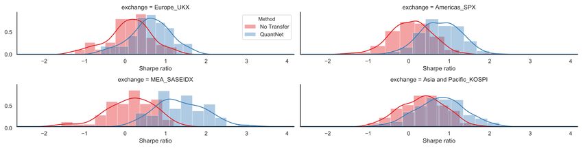
Figure 1: QuantNet workflow: from market data to decoding/signal generation.

[57, 78] like contagion effects and global macro-economic conditions that are crucial to accurately
capturing market movements that allow us to develop robust market trading strategies. Furthermore,
treating each market as an independent problem prevents effective use of machine learning since data
scarcity will cause models to overfit before learning useful trading strategies [82, 47, 22, 59].
Commonly-used techniques in machine learning such as transfer learning [15, 74, 101, 13], and
multi-task learning [15, 43, 13] could be used to handle information from multiple markets. However,
combining these techniques is not immediately evident because these approaches often presume
one task (market) as the main task and while others are auxiliary. When faced with several equally
essential tasks, a key problem is how to assign weights to each market loss when constructing a multi-
task objective. In our approach to end-to-end learning of global trading strategies, each market carries
equal weight. This poses a challenge because (a) markets are non-homogeneous (e.g., size, trading
days) and can cause interference during learning (e.g., errors from one market dominating others); (b)
the learning problem grows in complexity with each market, necessitating larger models that often
suffer from overfitting [27, 48] which is a notable problem in financial strategies [82, 47, 22, 59].
In this paper, we take a step towards overcoming these challenges and develop a full end-to-end
learning system for global financial trading. We introduce QuantNet: an architecture that learns
market-agnostic trends and uses them to learn superior market-specific trading strategies. Each
market-specific model is composed of an encoder-decoder pair (Figure 1). The encoder transforms
market-specific data into an abstract latent representation that is processed by a global model shared
by all markets, while the decoder learns a trading strategy based on the processed latent code returned
by the global model. QuantNet leverages recent insights from transfer and meta-learning that suggest
market-specific model components benefit from having separate parameters while being constrained
by conditioning on an abstract global representation [84]. Furthermore, by incorporating multiple
losses into a single network, our approach increases network regularization and avoids overfitting,
as in [62, 95, 13]. We evaluate QuantNet on historical data across 3103 assets in 58 global equity
markets. Against the best performing baseline Cross-sectional momentum [54, 9], QuantNet yields
51% higher Sharpe and 69% Calmar ratios. Also, we show the benefits of our approach, which
yields improvements of 15% and 41% in Sharpe and Calmar ratios, respectively, over the comparable
non-transfer learning variant.
Our key contributions are: (i) a novel architecture for transfer learning across financial trading
strategies; (ii) a novel learning objective to facilitate end-to-end training of trading strategies; and
(iii) demonstrate that QuantNet can achieve significant improvements across global markets with an
end-to-end learning system. To the best of our knowledge, this is the first paper that studies transfer
learning as a means of improving end-to-end large scale learning of trading strategies.

                                                   2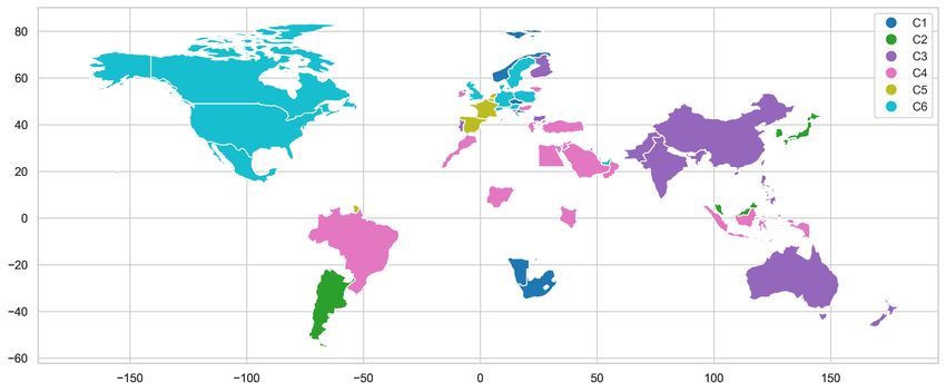
2     Related Work
Trading Strategies with Machine Learning Machine learning-based trading strategies have pre-
viously been explored in the setting of supervised learning [49, 2, 35, 85, 46] and reinforcement
learning [76, 66, 40, 104], nowadays with a major emphasis on deep learning methods. Broadly,
these works differ from our proposed method as they do not use inter-market knowledge transfer and
(in the case of methods based on supervised learning) tend to forecast returns/prices rather than to
generate end-to-end trading signals. We provide an in-depth treatment in Section 3.1.
Transfer Learning Transfer learning is a well-established method in machine learning [15, 74, 101].
It has been used in computer vision, medicine, and natural language processing [14, 58, 79]. In
financial systems, this paradigm has primarily been studied in the context of applying unstructured
data, such as social media, to financial predictions [3, 50]. In a few occasions such methodologies
have been applied to trading, usually combined with reinforcement learning and to a very limited
pool of assets [55]. We provide a thorough review of the area in appendix D.
The simplest and most common form of transfer learning pre-trains a model on a large dataset, hoping
that the pre-trained model can be fine-tuned to a new task or domain at a later stage [23, 67]. While
simple, this form of knowledge transfer assumes new tasks are similar to previous tasks, which
can easily fail in financial trading where markets differ substantially. Our method instead relies on
multi-task transfer learning [16, 8, 15, 83]. While this approach has previously been explored in a
financial context [42, 12], prior works either use full parameter sharing or share all but the final layer
of relatively simple models. In contrast, we introduce a novel architecture that relies on encoding
market-specific data into representations that pass through a global bottleneck for knowledge transfer.
We provide a detailed discussion in Section 3.2.

3     QuantNet
We begin by reviewing end-to-end learning of financial trading in section 3.1 and relevant forms of
transfer learning in section 3.2. We present our proposed architecture in section 3.3.

3.1   Preliminaries: Learning Trading Strategies

A financial market M = (a1 , . . . , an ) consists of a set of n assets aj ; at each discrete time step t
we have access to a vector of excess returns r t = (rt1 , . . . , rtn ) ∈ Rn . The goal of a trading strategy
f , parametrized by θ, is to map elements of a history Rm:t = (r t−m , . . . , r t ) into a set of trading
signals st = (s1t , . . . , snt ) ∈ Rn ; st = fθ (Rm:t ). These signals constitute a market portfolio: a trader
would buy one unit of an asset if sjt = 1, sell one unit if sjt = −1, and close a position if sjt = 0; any
value in between (−1, 1) implies that the trader is holding/shorting a fraction of an asset. The goal is
to produce a sequence of signals that maximize risk-adjusted returns. The most common approach is
to model f as a moving average parametrized by weights θ = (W1 , . . . , Wm ), Wi ∈ Rn×n , where
weights typically decreases exponentially or are hand-engineered and remain static [7, 4, 34];
                                                         t
                                                                   !
                                                       X
               sma                ma
                  t = τ (fθ (Rt−m:t )) = τ                   Wk r k , τ : Rn → [−1, 1]n .                   (1)
                                                  k=t−m

More advanced models rely on recurrence to form an abstract representation of the history up to time
t; either by using Kalman filtering, Hidden Markov Models (HMM), or Recurrent Neural Networks
(RNNs) [102, 35]. For our purposes, having an abstract representation of the history will be crucial
to facilitate effective knowledge transfer, as it captures each market’s dynamics, thereby allowing
QuantNet to disentangle general and idiosyncratic patterns. We use the Long Short-Term Memory
(LSTM) network [51, 41], which is a special form of an RNN. LSTMs have been recently explored to
form the core of trading strategy systems [35, 50, 85]. For simplicity, we present the RNN here and
refer the interested reader to [51, 41] or appendix C. The RNN is defined by introducing a recurrent
operation that updates a hidden representation h recurrently conditional on the input r:
        sRNN
         t   = τ (Ws ht + bs ),       ht = fθRNN (r t−1 , ht−1 ) = σ (Wr r t−1 + Wh ht−1 + b) ,            (2)
where σ is an element-wise activation function and θ = (Wr , Wh , b) parameterize the RNN. The
LSTM is similarly defined but adds a set of gating mechanisms to enhance the memory capacity

                                                      3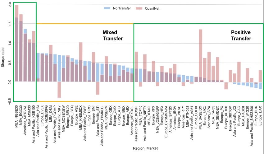
and gradient flow through the model. To learn the parameters of the RNN, we use truncated
backpropagation through time (TBPTT; [89]), which backpropagates a loss L through time to the
parameters of the RNN, truncating after K time steps.

3.2   Preliminaries: Transfer Learning

Transfer learning [15, 74, 83, 101] embodies a set of techniques for sharing information obtained
on one task, or market, when learning another task (market). In the simplest case of pre-training
[23, 67], for example, we would train a model in a market M2 by initializing its parameters to the
final parameters obtained in market M1 . While such pre-training can be useful, there is no guarantee
that the parameters obtain on task M1 will be useful for learning task M2 .
In multi-task transfer-learning, we have a set of M = (M1 , . . . , MN ) markets that we aim to learn
simultaneously. The multi-task literature often presumes one Mi is the main task, and all others are
auxiliary—their sole purpose is to improve final performance on Mi [15, 43]. A common problem in
                                how to assign weights wi to each market-specific loss Li when setting
multi-task transfer is thereforeP
the multi-task objective L = i wi Li . This is often a hyper-parameter that needs to be tuned [83].
As mentioned above, this poses a challenge in our case as markets are typically not homogeneous.
Instead, we turn to sequential multi-task transfer learning [84], which learns one model f i per market
Mi , but partition the parameters of the model into a set of market-specific parameters θi and a set
of market-agnostic parameters φ. In doing so, market-specific parameters are free to specialize on
the problem at hand, while market-agnostic parameters capture signals from all markets. However,
in contrast to standard approaches to multi-task transfer learning, which either share all parameters,
a set from the final layer(s) or share no parameters, we take inspiration from recent advances in
meta-learning [63, 107, 37], which shows that more flexible parameter-sharing schemes can reap
a greater reward. In particular, interleaving shared and market-specific parameters can be seen as
learning both shared representation and a shared optimizer [37].
We depart from previous work by introducing an encoder-decoder setup [18] within financial markets.
Encoders learn to represent market-specific information, such as internal fiscal and monetary condi-
tions, development stage, and so on, while a global shared model learns to represent market-agnostic
dynamics such as global economic outlook, contagion effects (via financial crises). The decoder uses
these sources of information to produce a market-specific trading strategy. With these preliminaries,
we now turn to QuantNet, our proposed method for end-to-end multi-market financial trading.

3.3   QuantNet

Architecture Figure 1 portrays the QuantNet architecture. In QuantNet, we associate each market
Mi with an encoder-decoder pair, where the encoder enci and the decoder deci are both LSTMs
networks. Both models maintain a separate hidden state, ei and di , respectively. When given a
market return vector r i , the encoder produces an encoding ei that is passed onto a market-agnostic
model ω, which modifies the market encoding into a representation z i :

                          z it = ω(eit ),   where   eit = enci (r it−1 , eit−1 ).                  (3)

Because ω is shared across markets, z i reflects market information from market M i while taking
global information (as represented by ω) into account. This bottleneck enforces local representations
that are aware of global dynamics, and so we would expect similar markets to exhibits similar
representations [70]. We demonstrate this empirically in Figure 2, which shows how each market is
being represented internally by QuantNet. We apply hierarchical clustering on hidden representation
from the encoder (see also dendrogram in appendix G) using six centroids. We observe clear
geo-economical structure emerging from QuantNet – without it receiving any such geographical
information. C5 consist mainly of small European equity markets (Spain, Netherlands, Belgium,
and France) – all neighbors; C6 encompass developed markets in Europe and Americas, such as
United Kingdom, Germany, US, and their respective neighbors Austria, Poland, Switzerland, Sweden,
Denmark, Canada, and Mexico. Other clusters are more refined: C2 for instance contains most
developed markets in Asia like Japan, Hong Kong, Korea, and Singapore, while C3 represents Asia
and Pacific emerging markets: China, India, Australia, and some respective neighbors (New Zealand,
Pakistan, Philippines, Taiwan).

                                                    4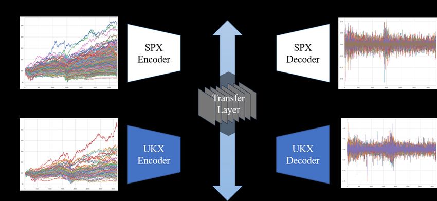
Figure 2: World map depicting the different clusters formed from the scores of QuantNet encoder. For
visualization purposes, we have picked the market with the biggest market capitalization to represent
the country in the cluster.

We experiment with different functional forms for ω; adding complexity to ω can allow more
sophisticated representations, but simpler architectures enforce an information bottleneck [100].
Indeed we find experimentally that a simple linear layer works better than an LSTM (see Appendix
H), which is in line with general wisdom on encoder-decoder architectures [19, 18].
Given a representation z it , we produce a market-specific trading strategy by decoding this abstract
representation into a hidden market-specific state dit ; this state represents the trading history in market
M i , along with the history of global dynamics, and is used learn a market-specific trading strategy
                  sit = f i (dit ) = tanh(W i dit + bi ),             where dit = deci (z it , dit−1 ).                   (4)
While f i can be any model, we found a simple linear layer sufficient due to the expressive capacity
of the encoder-decoder pair. For a well-behaved, non-leveraged trading strategy we chose tanh as
our activation function, which bounds the trading signal sit ∈ (−1, 1)n [1, 92].
From Eq. 4, we can see how transfer learning affects both trading and learning. During trading,
by processing a market encoding eit through a shared global layer ω, we impose a bottleneck such
that any trading strategy is forced to act on the globally conditioned information in z it . During
learning, market-specific trading is unrestricted in its parameter updates, but gradients are implicitly
modulated through the conditioned input. This is particularly true for the encoder, which must service
its corresponding decoder by passing through the global layer ω. Concretely, given a market loss
function Li with error signal δ i = dL/dsi , market-specific gradients are given by
                          ∂sit ∂ deci i i                                            ∂sit ∂dit ∂z it ∂ enci i i
  ∇θi i Li (sit ) = δti                (z t ; dt−1 ),   ∇θi i Li (sit ) = δti                               (r t ; et−1 ). (5)
     dec                  ∂dit ∂θdec
                                  i
                                     i                         enc                   ∂dit ∂z it ∂eit ∂θenc
                                                                                                        i
                                                                                                          i

The gradient of the decoder is largely free but must adapt to the representation produced by the
encoder and the global model. These, in turn, are therefore influenced by what representations are
useful for the decoder. In particular, the gradient of the encoder must pass through the global model,
which acts as a preconditioner of the encoder parameter gradient, thereby encoding an optimizer [36].
Finally, to see how global information gets encoded in the global model, under a multi-task loss, its
gradients effectively integrate out idiosyncratic market correlations:
                                                               n
                                                               X           ∂sit ∂dit ∂ω i
                                  ∇φ L(s1t , . . . , snt ) =         δti                 (et ).                           (6)
                                                               i=1
                                                                           ∂dit ∂z it ∂φ

Learning Objective To effectively learn trading strategies with QuantNet, we develop a novel
learning objective based on the Sharpe ratio [86, 5, 47]. Prior work on financial forecast tends to
rely on Mean Squared Error (MSE) [49, 50, 46], as does most work on learning trading strategies.
A few works have instead considered other measurements [35, 102, 104]. In particular, there are

                                                                5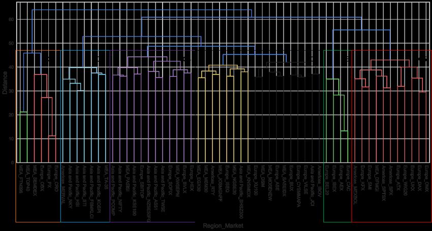
Algorithm 1 QuantNet Training
Require: Markets M = (M1 , . . . MN )
Require: Backpropagation horizon k
 1: while True do
 2:    Sample mini-batch M of m markets from M
 3:    Randomly select t ∈ 1, . . . , T
 4:    Compute encodings eit−k:t , z it−k:t , and dit−k:t for all Mi ∈ M                           Eqs. 3 and 4
 5:    Compute signals sit−k:t for all Mi ∈ M                                                             Eq. 4
 6:    Compute Sharpe ratios ρit:j for all assets aij ∈ Mi and markets Mi ∈ M                             Eq. 7

                                                       N
 7:    Compute QuantNet loss L {sit−k:t , r it−k:t }i=1                                                   Eq. 8
 8:    Update model parameters by truncated backpropagation through time                           Eqs. 5 and 6
 9: end while

strong theoretical and empirical reasons for considering the Sharpe ratio instead of MSE – in fact,
MSE minimization is a necessary, but not sufficient condition to maximize the profitability of a
trading strategy [10, 1, 60]. Since some assets are more volatile than others, the Sharpe ratio helps to
discount the optimistic average returns by taking into account the risk faced when traded those assets.
Also, it is widely adopted by quantitative investment strategists to rank different strategies and funds
[86, 5, 47].
To compute each market Sharpe ratio at a time t, truncated to backpropagation through time for k
steps (to t − k), considering excess daily returns, we first compute the per-asset Sharpe ratio
                                                               √
                                ρit,j = µit−k:t,j
                                                   i
                                                     σt−k:t,j · 252,                            (7)

where µit,j is the average return of the strategy for asset j and σtj is its respective the standard
                √
deviation. The 252 factor is included in computing the annualized Sharpe ratio. The market loss
function and the QuantNet objective are given by averaging over assets and markets, respectively:
                                      N                                                           n
                            N
                                  1 X i i                                                      1X i
      L {sit−k:t , r it−k:t }i=1 =       L (st−k:t , r it−k:t ),   Li (sit−k:t , r it−k:t ) =        ρ ,    (8)
                                   N i=1                                                        n j=1 t,j

Training To train QuantNet, we use stochastic gradient descent. To obtain a gradient update, we
first sample mini-batches of m markets from the full set M = (M1 , . . . , MN ) to obtain an empirical
expectation over markets. Given these, we randomly sample a time step t and run the model from
t − k to t, from which we obtain market Sharpe ratios. Then, we compute QuantNet loss function and
differentiate through time into all parameters. We pass this gradient to an optimizer, such as Adam,
to take one step on the model’s parameters. This process is repeated until the model converges.

4     Results
This section assesses QuantNet performance compared to baselines and a No Transfer strategy defined
by a single LSTM of the same dimensionality as the decoder architecture (number of assets), as
defined in Eq. 2. Next section presents the main experimental setting, with the subsequent ones
providing: (i) a complete comparison of QuantNet with other trading strategies; (ii) an in-depth
comparison of QuantNet versus the best No Transfer strategy; and (iii) analysis on market conditions
that facilitate transfer under QuantNet. We provide an ablation study and sensitivity analysis of
QuantNet in appendix H.

4.1     Experimental Setting

Datasets Appendix A provides a full table listing all 58 markets used. We tried to find a compromise
between the number of assets and sample size, hence for most markets, we were unable to use the
full list of constituents. We aimed to collect daily price data ranging from 03/01/2000 to 15/03/2019,
but for most markets it starts roughly around 2010. Finally, due to restrictions from our Bloomberg
license, we were unable to access data for some important equity markets, such as Italy and Russia.

                                                      6
Evaluation Appendix B provides full experimental details, including detailed descriptions of
baselines and hyperparameter search protocols. We report results for trained models under best
hyperparameters on validation sets; for each dataset we construct a training and validation set, where
the latter consists of the last 752 observations of each time series (around 3 years). We have used 3
Month London Interbank Offered Rate in US Dollar as the reference rate to compute excess returns.
We have also reported Calmar ratios, Annualized Returns and Volatility, Downside risk, Sortino
ratios, Skewness and Maximum drawdowns [99, 86, 28, 81].
4.2 Empirical Evaluation
Baseline Comparison Table 1 present median and mean absolute deviation (in brackets) perfor-
mance of the different trading strategies on 3103 stocks across all markets analysed. The best
baseline is Cross-sectional Momentum (CS Mom), yielding a SR of 0.23 and CR of 0.14. QuantNet
outperforms CS Mom, yielding 51% higher SR and 69% higher CR. No Transfer LSTM and Linear
outperforms this baseline as well, but not to the same extent as QuantNet.
Table 1: Median and mean absolute deviation (in brackets) performance on 3103 stocks across all
markets analysed. TS Mom - Time series momentum and CS Mom - Cross-section momentum. We
highlighted in bold only the metrics where a comparison can be made, like Sharpe ratios, Calmar
ratios, Kurtosis, Skewness, and Sortino ratios.
Metric Buy and hold Risk parity TS Mom CS Mom No Transfer LSTM No Transfer Linear QuantNet
Ann Ret 0.000020 0.000193 0.000050 0.000042 0.002508 0.001537 0.005377
(0.13433) (0.00270) (0.00019) (0.00019) (0.07645) (0.08634) (0.02898)
Ann Vol 0.287515 0.001536 0.000290 0.000270 0.008552 0.007768 0.023665
(0.10145) (0.00537) (0.00036) (0.00036) (0.13455) (0.14108) (0.04540)
CR 0.000040 0.095516 0.139599 0.143195 0.158987 0.169345 0.241255
(0.33583) (0.29444) (1.05288) (1.18751) (0.55762) (0.57170) (0.59968)
DownRisk 0.202361 0.001076 0.000195 0.000178 0.005656 0.005124 0.015734
(0.07042) (0.00361) (0.00024) (0.00025) (0.09223) (0.09553) (0.03291)
Kurt 5.918386 6.165916 13.333863 18.112853 16.87256 15.73864 16.19961
(10.2515) (13.9426) (19.2278) (24.4672) (30.2204) (31.0395) (24.7336)
MDD -0.419984 -0.002935 -0.000488 -0.000444 -0.014564 -0.01286 -0.03847
(0.14876) (0.00987) (0.00082) (0.00081) (0.16724) (0.17820) (0.07881)
SR 0.000051 0.155560 0.226471 0.234583 0.304244 0.306572 0.354776
(0.42324) (0.42028) (0.40627) (0.41547) (0.51552) (0.51182) (0.57218)
Skew -0.087282 -0.092218 0.427237 0.568364 0.256736 0.171629 0.297182
(0.82186) (0.96504) (1.28365) (1.60612) (1.77245) (1.74804) (1.66854)
SortR 0.217621 0.220335 0.333685 0.349124 0.443422 0.454035 0.52196
(0.59710) (0.61883) (1.02616) (0.633953) (0.78525) (0.86715) (1.02465)
Figure 3: Histogram of Sharpe ratio contrasting QuantNet with baseline strategies.
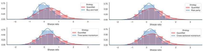
QuantNet vs No Transfer Linear When comparing QuantNet and No Transfer Linear strategies
performance (Table 1), we observe an improvement of about 15% on SR and 41% on CR. This
improvement increases the number of assets yielding SRs above 1.0 from 432 to 583, smaller Down-
side Risk (DownRisk), higher Skew and Sortino ratios (SortR). Statistically, QuantNet significantly
outperform No Transfer both in Sharpe (W = 2215630, p-value < 0.01) and Calmar (W = 2141782,
p-value < 0.01) ratios. This discrepancy manifests in statistical terms, with the Kolmogorov-Smirnov
statistic indicating that these distributions are meaningfully different (KS = 0.053, p-value < 0.01).
Figure 4 outlines the average SR across the 58 markets, ordered by No Transfer strategy performance.
In SR terms, QuantNet outperforms No Transfer in its top 5 markets and dominates the bottom 10
7markets where No Transfer yields negative results, both in terms of SR and CR ratios. Finally, in 7 of
the top 10 largest ones (RTY, SPX, KOSPI, etc.), QuantNet also outperforms No Transfer. Figure
5a presents cumulative returns charts in a set of large regional markets, such as United States S&P
500 components (SPX Index), United Kingdom FTSE 100 (UKX Index), Korea Composite Index
(KOSPI Index) and Saudi Arabia Tadawul All Shares (SASEIDX Index). Across regions, we observe
a 2-10 times order of magnitude improvement in SRs and CRs by QuantNet, with similar benefits in
Sortino ratios, Downside risks, and Skewness. Appendix E provides further analysis.
Figure 4: Average Sharpe ratios of QuantNet and No Transfer across 58 equity markets.
(b)
(a) (c)
Figure 5: (a) Average cumulative returns (%) of SPX Index, UKX Index, KOSPI Index and SASEIDX
Index contrasting QuantNet and No Transfer. Average Sharpe ratio difference between QuantNet
versus No Transfer, aggregated by sample size (b) and number of assets per market (c) – in both we
have subtracted QuantNet SR from No Transfer SR to reduce cross-asset variance and baseline effect.
QuantNet Features One of the key features of transfer learning is its ability to provide meaningful
solutions in resource-constrained scenarios – sample size, features, training budget, etc. With
8QuantNet this pattern persists; Figure 5b presents the average SR grouped based on market sample
size in the training set. As transfer-learning would predict, we observe large gains to transfer in
markets with tiny sample size (1444-1823 samples or 6-7 years) where fitting a model on only local
market data yields poor performance. Further, gains from transfer generally decay as sample sizes
increase. Interestingly, we find that medium-sized markets (2200-2576 samples or 10 years of data)
do not benefit from transfer, suggesting that there is room for improvement in the design of our
transfer bottleneck ω, an exciting avenue for future research. Another vital feature is coping with
market size – Figure 5c outlines QuantNet performance in terms of average SR. It demonstrates that
the bigger the market, the better QuantNet will perform.
5 Conclusion
In this paper, we introduce QuantNet: an architecture that learns market-agnostic trends and use these
to learn superior market-specific trading strategies. QuantNet uses recent advances in transfer- and
meta-learning, where market-specific parameters are free to specialize on the problem at hand, while
market-agnostic parameters capture signals from all markets. QuantNet takes a step towards end-to-
end global financial trading that can deliver superior market returns. In a few big regional markets,
such as S&P 500, FTSE 100, KOSPI and Saudi Arabia Tadawul All Shares, QuantNet showed 2-10
times improvement in SR and CR. QuantNet also generated positive and statistically significant alpha
according to Fama-French 5 factors model (appendix F). An avenue of future research is to identify
the functional form of a global transfer layer that can deliver strong performance also on markets
where mixed transfer occurred, such as those with medium sample size.
Broader Impact
As this work proposes a machine learning system for financial trading, there are potential societal
impacts. In principle, research that creates systems capable of matching expert trading performance
provides a social good in that it can democratize financial trading. This is provided that the system
can be trained (or is provided pre-trained) and can be deployed by individuals. Conversely, there are
potential societal issues to technological advancements in financial trading; as system specialize and
become increasingly complex, it is conceivable that they become less inclusive in their applicability,
more opaque, and increase systemic risk.
We believe that while these potential benefits and risks apply in principle to our broad research
direction, QuantNet itself is unlikely to have a significant societal impact. First, it is not meant for
personal trading in its current form, and we provide no interface through which individuals or entities,
in general, can make financial decisions. Second, QuantNet relies on well-known components,
namely LSTMs, feed-forward networks, and stochastic gradient descent - all of which can be built
with open-source software and trained on personal hardware. Hence we believe that QuantNet is
widely accessible to the general public.
References
[1] Emmanuel Acar and Stephen Satchell. Advanced trading rules. Butterworth-Heinemann,
2002.
[2] Saurabh Aggarwal and Somya Aggarwal. Deep investment in financial markets using deep
learning models. International Journal of Computer Applications, 162(2):40–43, 2017.
[3] Dogu Araci. Finbert: Financial sentiment analysis with pre-trained language models. arXiv
preprint arXiv:1908.10063, 2019.
[4] A Avramovic, V Lin, and M Krishnan. We’re all high frequency traders now. Credit Suisse
Market Structure White Paper, 2017.
[5] David H Bailey and Marcos Lopez de Prado. The sharpe ratio efficient frontier. Journal of
Risk, 15(2):13, 2012.
[6] Markus Baltzer, Stephan Jank, and Esad Smajlbegovic. Who trades on momentum? Journal
of Financial Markets, 42:56–74, 2019.
9[7] BarclayHedge. Barclayhedge: Cta’s asset under management. Available on-
line at https: // www. barclayhedge. com/ research/ indices/ cta/ Money_ Under_
Management. html , 2017.
[8] Jonathan Baxter. Learning internal representations. In Proceedings of the eighth annual
conference on Computational learning theory, pages 311–320, 1995.
[9] Jamil Baz, Nicolas Granger, Campbell R Harvey, Nicolas Le Roux, and Sandy Rattray.
Dissecting investment strategies in the cross section and time series. Available at SSRN
2695101, 2015.
[10] Yoshua Bengio. Using a financial training criterion rather than a prediction criterion. Interna-
tional Journal of Neural Systems, 8(04):433–443, 1997.
[11] James Bergstra and Yoshua Bengio. Random search for hyper-parameter optimization. Journal
of Machine Learning Research, 13(Feb):281–305, 2012.
[12] Zsolt Bitvai and Trevor Cohn. Day trading profit maximization with multi-task learning and
technical analysis. Machine Learning, 101(1-3):187–209, 2015.
[13] Stefano B. Blumberg, Marco Palombo, Can Son Khoo, Chantal M. W. Tax, Ryutaro Tanno,
and Daniel C. Alexander. Multi-stage prediction networks for data harmonization. In Medical
image computing and computer assisted interventaion, pages 411–419, 2019.
[14] Stefano B Blumberg, Ryutaro Tanno, Iasonas Kokkinos, and Daniel C Alexander. Deeper
image quality transfer: Training low-memory neural networks for 3d images. In International
Conference on Medical Image Computing and Computer-Assisted Intervention, pages 118–125.
Springer, 2018.
[15] Rich Caruana. Multitask learning. Machine learning, 28(1):41–75, 1997.
[16] Richard Caruana. Multitask learning: A knowledge-based source of inductive bias. In
Proceedings of the Tenth International Conference on Machine Learning, pages 41–48. Morgan
Kaufmann, 1993.
[17] Sihong Chen, Kai Ma, and Yefeng Zheng. Med3d: Transfer learning for 3d medical image
analysis. arXiv preprint arXiv:1904.00625, 2019.
[18] KyungHyun Cho, Bart van Merrienboer, Dzmitry Bahdanau, and Yoshua Bengio. On the
properties of neural machine translation: Encoder-decoder approaches. CoRR, abs/1409.1259,
2014.
[19] Kyunghyun Cho, Bart van Merriënboer, Caglar Gulcehre, Dzmitry Bahdanau, Fethi Bougares,
Holger Schwenk, and Yoshua Bengio. Learning phrase representations using rnn encoder–
decoder for statistical machine translation. In Proceedings of the 2014 Conference on Empirical
Methods in Natural Language Processing (EMNLP), pages 1724–1734, 2014.
[20] Yves Choueifaty and Yves Coignard. Toward maximum diversification. The Journal of
Portfolio Management, 35(1):40–51, 2008.
[21] Kent Daniel and Tobias J Moskowitz. Momentum crashes. Journal of Financial Economics,
122(2):221–247, 2016.
[22] Marcos Lopez De Prado. Advances in financial machine learning. John Wiley & Sons, 2018.
[23] Jacob Devlin, Ming-Wei Chang, Kenton Lee, and Kristina Toutanova. Bert: Pre-training of
deep bidirectional transformers for language understanding. arXiv preprint arXiv:1810.04805,
2018.
[24] Jacob Devlin, Ming-Wei Chang, Kenton Lee, and Kristina Toutanova. Bert: Pre-training of
deep bidirectional transformers for language understanding. arXiv preprint arXiv:1810.04805,
2018.
[25] Hubert Dichtl. Investing in the s&p 500 index: Can anything beat the buy-and-hold strategy?
Review of Financial Economics, 38(2):352–378, 2020.
[26] Johan Du Plessis and Winfried G Hallerbach. Volatility weighting applied to momentum
strategies. The Journal of Alternative Investments, 19(3):40–58, 2016.
[27] Salam El Bsat, Haitham Bou Ammar, and Matthew E Taylor. Scalable multitask policy gradient
reinforcement learning. In Thirty-First AAAI Conference on Artificial Intelligence, 2017.
10[28] Martin Eling and Frank Schuhmacher. Does the choice of performance measure influence the
evaluation of hedge funds? Journal of Banking & Finance, 31(9):2632–2647, 2007.
[29] Edwin J Elton, Martin J Gruber, and Andre de Souza. Passive mutual funds and etfs: Perfor-
mance and comparison. Journal of Banking & Finance, 106:265–275, 2019.
[30] Tatiana Escovedo, Adriano Koshiyama, Andre Abs da Cruz, and Marley Vellasco. Detecta:
abrupt concept drift detection in non-stationary environments. Applied Soft Computing,
62:119–133, 2018.
[31] Eugene F Fama and Kenneth R French. A five-factor asset pricing model. Journal of financial
economics, 116(1):1–22, 2015.
[32] Li Fei-Fei, Rob Fergus, and Pietro Perona. One-shot learning of object categories. IEEE
transactions on pattern analysis and machine intelligence, 28(4):594–611, 2006.
[33] Guanhao Feng, Stefano Giglio, and Dacheng Xiu. Taming the factor zoo: A test of new factors.
The Journal of Finance, 75(3):1327–1370, 2020.
[34] Nick Firoozye and Adriano Koshiyama. Optimal dynamic strategies on gaussian returns.
Available at SSRN 3385639, 2019.
[35] Thomas Fischer and Christopher Krauss. Deep learning with long short-term memory networks
for financial market predictions. European Journal of Operational Research, 270(2):654–669,
2018.
[36] Sebastian Flennerhag, Andrei A. Rusu, Razvan Pascanu, Francesco Visin, Hujun Yin, and
Raia Hadsell. Meta-learning with warped gradient descent. In International Conference on
Learning Representations, 2020.
[37] Sebastian Flennerhag, Andrei A Rusu, Razvan Pascanu, Franscesco Visin, Hujun Yin, and
Raia Hadsell. Meta-learning with warped gradient descent. In International Conference on
Learning Representations, 2020.
[38] Sebastian Flennerhag, Hujun Yin, John Keane, and Mark Elliot. Breaking the activation
function bottleneck through adaptive parameterization. In Advances in Neural Information
Processing Systems, pages 7739–7750, 2018.
[39] Kenneth R French. Kenneth r. french-data library. Tuck-MBA program web server. http://mba.
tuck. dartmouth. edu/pages/faculty/ken. french/data_library. html (accessed October 20, 2010),
2012.
[40] Ziming Gao, Yuan Gao, Yi Hu, Zhengyong Jiang, and Jionglong Su. Application of deep
q-network in portfolio management. arXiv preprint arXiv:2003.06365, 2020.
[41] Felix A Gers, Jürgen Schmidhuber, and Fred Cummins. Learning to forget: Continual
prediction with lstm. 1999.
[42] Joumana Ghosn and Yoshua Bengio. Multi-task learning for stock selection. In Advances in
neural information processing systems, pages 946–952, 1997.
[43] Andrew Gibiansky, Sercan Arik, Gregory Diamos, John Miller, Kainan Peng, Wei Ping,
Jonathan Raiman, and Yanqi Zhou. Deep voice 2: Multi-speaker neural text-to-speech. In
Advances in neural information processing systems, pages 2962–2970, 2017.
[44] Xavier Glorot, Antoine Bordes, and Yoshua Bengio. Domain adaptation for large-scale
sentiment classification: A deep learning approach. In Proceedings of the 28th international
conference on machine learning (ICML-11), pages 513–520, 2011.
[45] Ian Goodfellow, Yoshua Bengio, and Aaron Courville. Deep learning. MIT press, 2016.
[46] Shihao Gu, Bryan Kelly, and Dacheng Xiu. Empirical asset pricing via machine learning. The
Review of Financial Studies, 33(5):2223–2273, 2020.
[47] Campbell R Harvey and Yan Liu. Backtesting. The Journal of Portfolio Management, pages
12–28, 2015.
[48] Xiao He, Francesco Alesiani, and Ammar Shaker. Efficient and scalable multi-task regression
on massive number of tasks. In Proceedings of the AAAI Conference on Artificial Intelligence,
volume 33, pages 3763–3770, 2019.
[49] James B Heaton, Nick G Polson, and Jan Hendrik Witte. Deep learning for finance: deep
portfolios. Applied Stochastic Models in Business and Industry, 33(1):3–12, 2017.
11[50] Joshua Zoen Git Hiew, Xin Huang, Hao Mou, Duan Li, Qi Wu, and Yabo Xu. Bert-
based financial sentiment index and lstm-based stock return predictability. arXiv preprint
arXiv:1906.09024, 2019.
[51] Sepp Hochreiter and Jürgen Schmidhuber. Long short-term memory. Neural computation,
9(8):1735–1780, 1997.
[52] Yong Hu, Kang Liu, Xiangzhou Zhang, Kang Xie, Weiqi Chen, Yuran Zeng, and Mei Liu.
Concept drift mining of portfolio selection factors in stock market. Electronic Commerce
Research and Applications, 14(6):444–455, 2015.
[53] Allendbridge IS. Quantitative investment strategy survey. Pensions & Investments, 2014.
[54] Narasimhan Jegadeesh and Sheridan Titman. Returns to buying winners and selling losers:
Implications for stock market efficiency. The Journal of finance, 48(1):65–91, 1993.
[55] Gyeeun Jeong and Ha Young Kim. Improving financial trading decisions using deep q-learning:
Predicting the number of shares, action strategies, and transfer learning. Expert Systems with
Applications, 117:125–138, 2019.
[56] Shuhui Jiang, Haiyi Mao, Zhengming Ding, and Yun Fu. Deep decision tree transfer boosting.
IEEE transactions on neural networks and learning systems, 2019.
[57] Dror Y Kenett, Matthias Raddant, Lior Zatlavi, Thomas Lux, and Eshel Ben-Jacob. Corre-
lations and dependencies in the global financial village. In International Journal of Modern
Physics: Conference Series, volume 16, pages 13–28. World Scientific, 2012.
[58] Simon Kornblith, Jonathon Shlens, and Quoc V Le. Do better imagenet models transfer better?
In Proceedings of the IEEE conference on computer vision and pattern recognition, pages
2661–2671, 2019.
[59] Adriano Koshiyama and Nick Firoozye. Avoiding backtesting overfitting by covariance-
penalties: an empirical investigation of the ordinary and total least squares cases. The Journal
of Financial Data Science, 1(4):63–83, 2019.
[60] Adriano Koshiyama and Nick Firoozye. Avoiding backtesting overfitting by covariance-
penalties: an empirical investigation of the ordinary and total least squares cases. The Journal
of Financial Data Science, 1(4):63–83, 2019.
[61] Wouter Marco Kouw and Marco Loog. A review of domain adaptation without target labels.
IEEE transactions on pattern analysis and machine intelligence, 2019.
[62] Chen-Yu Lee, Saining Xie, Patrick Gallagher, Zhengyou Zhang, and Zhuowen Tu. Deeply-
supervised nets. International Conference on Artificial Intelligence and Statistics, 2015.
[63] Yoonho Lee and Seungjin Choi. Gradient-based meta-learning with learned layerwise metric
and subspace. arXiv preprint arXiv:1801.05558, 2018.
[64] Wei Li, Shuai Ding, Yi Chen, and Shanlin Yang. A transfer learning approach for credit
scoring. In International Conference on Applications and Techniques in Cyber Security and
Intelligence, pages 64–73. Springer, 2018.
[65] Xiaodong Li, Haoran Xie, Raymond YK Lau, Tak-Lam Wong, and Fu-Lee Wang. Stock
prediction via sentimental transfer learning. IEEE Access, 6:73110–73118, 2018.
[66] Yuming Li, Pin Ni, and Victor Chang. Application of deep reinforcement learning in stock
trading strategies and stock forecasting. Computing, pages 1–18, 2019.
[67] Yinhan Liu, Myle Ott, Naman Goyal, Jingfei Du, Mandar Joshi, Danqi Chen, Omer Levy,
Mike Lewis, Luke Zettlemoyer, and Veselin Stoyanov. Roberta: A robustly optimized bert
pretraining approach. arXiv preprint arXiv:1907.11692, 2019.
[68] Zongying Liu, Chu Kiong Loo, and Manjeevan Seera. Meta-cognitive recurrent recursive
kernel os-elm for concept drift handling. Applied Soft Computing, 75:494–507, 2019.
[69] Lionel Martellini. Toward the design of better equity benchmarks: Rehabilitating the tangency
portfolio from modern portfolio theory. The Journal of Portfolio Management, 34(4):34–41,
2008.
[70] Tomas Mikolov, Ilya Sutskever, Kai Chen, Greg S Corrado, and Jeff Dean. Distributed
representations of words and phrases and their compositionality. In Advances in neural
information processing systems, pages 3111–3119, 2013.
12[71] Marat Molyboga. Portfolio management of commodity trading advisors with volatility target-
ing. Available at SSRN 3123092, 2018.
[72] Tobias J Moskowitz, Yao Hua Ooi, and Lasse Heje Pedersen. Time series momentum. Journal
of financial economics, 104(2):228–250, 2012.
[73] Manuel Nunes, Enrico Gerding, Frank McGroarty, and Mahesan Niranjan. A comparison of
multitask and single task learning with artificial neural networks for yield curve forecasting.
Expert Systems with Applications, 119:362–375, 2019.
[74] Sinno Jialin Pan and Qiang Yang. A survey on transfer learning. IEEE Transactions on
knowledge and data engineering, 22(10):1345–1359, 2009.
[75] Wonpyo Park, Dongju Kim, Yan Lu, and Minsu Cho. Relational knowledge distillation. In
The IEEE Conference on Computer Vision and Pattern Recognition (CVPR), June 2019.
[76] Parag C Pendharkar and Patrick Cusatis. Trading financial indices with reinforcement learning
agents. Expert Systems with Applications, 103:1–13, 2018.
[77] Chen Qu, Feng Ji, Minghui Qiu, Liu Yang, Zhiyu Min, Haiqing Chen, Jun Huang, and W Bruce
Croft. Learning to selectively transfer: Reinforced transfer learning for deep text matching. In
Proceedings of the Twelfth ACM International Conference on Web Search and Data Mining,
pages 699–707. ACM, 2019.
[78] Matthias Raddant and Dror Y Kenett. Interconnectedness in the global financial market. OFR
WP, pages 16–09, 2016.
[79] Alec Radford, Jeffrey Wu, Rewon Child, David Luan, Dario Amodei, and Ilya Sutskever.
Language models are unsupervised multitask learners. OpenAI Blog, 1(8):9, 2019.
[80] Sashank J Reddi, Satyen Kale, and Sanjiv Kumar. On the convergence of adam and beyond.
arXiv preprint arXiv:1904.09237, 2019.
[81] Tom Rollinger and Scott Hoffman. Sortino ratio: A better measure of risk. Futures Magazine,
1(02), 2013.
[82] Joseph P Romano and Michael Wolf. Stepwise multiple testing as formalized data snooping.
Econometrica, 73(4):1237–1282, 2005.
[83] Sebastian Ruder. An overview of multi-task learning in deep neural networks. arXiv preprint
arXiv:1706.05098, 2017.
[84] Sebastian Ruder, Matthew E Peters, Swabha Swayamdipta, and Thomas Wolf. Transfer
learning in natural language processing. In Proceedings of the 2019 Conference of the North
American Chapter of the Association for Computational Linguistics: Tutorials, pages 15–18,
2019.
[85] Omer Berat Sezer, Mehmet Ugur Gudelek, and Ahmet Murat Ozbayoglu. Financial time
series forecasting with deep learning: A systematic literature review: 2005–2019. Applied Soft
Computing, 90:106181, 2020.
[86] William F Sharpe. The sharpe ratio. Journal of portfolio management, 21(1):49–58, 1994.
[87] Richard Socher, Milind Ganjoo, Christopher D Manning, and Andrew Ng. Zero-shot learning
through cross-modal transfer. In Advances in neural information processing systems, pages
935–943, 2013.
[88] Akila Somasundaram and Srinivasulu Reddy. Parallel and incremental credit card fraud detec-
tion model to handle concept drift and data imbalance. Neural Computing and Applications,
31(1):3–14, 2019.
[89] Ilya Sutskever. Training Recurrent Neural Networks. PhD thesis, CAN, 2013.
[90] Andreas Thomann. Factor-based tactical bond allocation and interest rate risk management.
Available at SSRN 3122096, 2019.
[91] Lisa Torrey and Jude Shavlik. Transfer learning. In Handbook of research on machine learning
applications and trends: algorithms, methods, and techniques, pages 242–264. IGI Global,
2010.
[92] Johannes Voit. The statistical mechanics of financial markets. Springer Science & Business
Media, 2013.
13[93] Andrew Voumard and Ghassan Beydoun. Transfer learning in credit risk. In ECML PKDD,
pages 1–16, 2019.
[94] Donghui Wang, Yanan Li, Yuetan Lin, and Yueting Zhuang. Relational knowledge transfer for
zero-shot learning. In Proceedings of the Thirtieth AAAI Conference on Artificial Intelligence,
AAAI’16, pages 2145–2151. AAAI Press, 2016.
[95] Liwei Wang, Chen-Yu Lee, Zhuowen Tu, and Svetlana Lazebnik. Training deeper convolutional
networks with deep supervision. arxiv arXiv: 1505. 02496 , 2015.
[96] Wei Wang, Vincent W Zheng, Han Yu, and Chunyan Miao. A survey of zero-shot learning:
Settings, methods, and applications. ACM Transactions on Intelligent Systems and Technology
(TIST), 10(2):13, 2019.
[97] Yaqing Wang, Quanming Yao, James Kwok, and Lionel M. Ni. Generalizing from a few
examples: A survey on few-shot learning, 2019.
[98] Zhilin Yang, Jake Zhao, Bhuwan Dhingra, Kaiming He, William W Cohen, Ruslan R Salakhut-
dinov, and Yann LeCun. Glomo: unsupervised learning of transferable relational graphs. In
Advances in Neural Information Processing Systems, pages 8950–8961, 2018.
[99] Terry W Young. Calmar ratio: A smoother tool. Futures, 20(1):40, 1991.
[100] Shujian Yu and Jose C Principe. Understanding autoencoders with information theoretic
concepts. Neural Networks, 117:104–123, 2019.
[101] Lei Zhang. Transfer adaptation learning: A decade survey. arXiv preprint arXiv:1903.04687,
2019.
[102] Mengqi Zhang, Xin Jiang, Zehua Fang, Yue Zeng, and Ke Xu. High-order hidden markov
model for trend prediction in financial time series. Physica A: Statistical Mechanics and its
Applications, 517:1–12, 2019.
[103] Yu Zhang and Qiang Yang. A survey on multi-task learning. arXiv preprint arXiv:1707.08114,
2017.
[104] Zihao Zhang, Stefan Zohren, and Stephen Roberts. Deep reinforcement learning for trading.
The Journal of Financial Data Science, 2(2):25–40, 2020.
[105] Fuzhen Zhuang, Xiaohu Cheng, Ping Luo, Sinno Jialin Pan, and Qing He. Supervised repre-
sentation learning: Transfer learning with deep autoencoders. In Twenty-Fourth International
Joint Conference on Artificial Intelligence, 2015.
[106] Fuzhen Zhuang, Zhiyuan Qi, Keyu Duan, Dongbo Xi, Yongchun Zhu, Hengshu Zhu,
Hui Xiong, and Qing He. A comprehensive survey on transfer learning. arXiv preprint
arXiv:1911.02685, 2019.
[107] Luisa M Zintgraf, Kyriacos Shiarlis, Vitaly Kurin, Katja Hofmann, and Shimon Whiteson.
Fast context adaptation via meta-learning. arXiv preprint arXiv:1810.03642, 2018.
[108] Indrė Žliobaitė, Mykola Pechenizkiy, and Joao Gama. An overview of concept drift appli-
cations. In Big data analysis: new algorithms for a new society, pages 91–114. Springer,
2016.
14A Datasets
Table 2 presents the datasets/markets used to empirically evaluate QuantNet. All the data was
obtained via Bloomberg, with the description of each market/index and its constituents at https:
//www.bloomberg.com; for instance, SPX can be found by searching using the following link
https://www.bloomberg.com/quote/SPX:IND. We tried to find a compromise between number
of assets and sample size, hence for most markets we were unable to use the full list of constituents.
We aimed to collect daily price data ranging from 03/01/2000 to 15/03/2019, but for most markets it
starts roughly around 2010. Finally, due to restrictions from our Bloomberg license, we were unable
to access data for some important equity markets, such as Italy and Russia. Full list with assets
and respective exchange can be found at: https://www.dropbox.com/s/eobhg2w8ithbgsp/
AssetsExchangeList.xlsx?dl=0
Table 2: Markets used during our experiment. MEA - Middle East and Africa.
Region Index/Market Country # Samples # Assets Region Index/Market Country # Samples # Assets
Americas IBOV Brazil 3250 29 Europe HEX Finland 1882 65
Americas MERVAL Argentina 3055 11 Europe IBEX Spain 3499 23
Americas MEXBOL Mexico 3002 19 Europe ISEQ Ireland 2888 14
Americas RTY US 2356 554 Europe KFX Denmark 3345 15
Americas SPTSX Canada 3173 129 Europe OBX Norway 2812 17
Americas SPX US 3291 376 Europe OMX Sweden 3453 29
Asia and Pacific AS51 Australia 2363 91 Europe PX Czechia 3374 5
Asia and Pacific FBMKLCI Malaysia 3131 23 Europe SBITOP Slovenia 2995 6
Asia and Pacific HSI China 2599 37 Europe SMI Switzerland 3948 19
Asia and Pacific JCI Indonesia 2007 44 Europe SOFIX Bulgaria 1833 5
Asia and Pacific KOSPI South Korea 3041 297 Europe UKX UK 3664 75
Asia and Pacific KSE100 Pakistan 2036 41 Europe VILSE Lithuania 2765 5
Asia and Pacific NIFTY India 3066 38 Europe WIG20 Poland 3449 8
Asia and Pacific NKY Japan 3504 186 Europe XU100 Turkey 2545 76
Asia and Pacific NZSE50FG New Zealand 3258 21 MEA DFMGI UAE 2184 11
Asia and Pacific PCOMP Philippines 3013 16 MEA DSM Qatar 2326 16
Asia and Pacific SHSZ300 China 2881 18 MEA EGX30 Egypt 1790 22
Asia and Pacific STI Singapore 2707 27 MEA FTN098 Namibia 1727 16
Asia and Pacific TWSE Taiwan 3910 227 MEA JOSMGNFF Jordan 2287 15
Europe AEX Netherlands 4083 17 MEA KNSMIDX Kenya 1969 14
Europe ASE Greece 2944 51 MEA KWSEPM Kuwait 2785 11
Europe ATX Austria 3511 13 MEA MOSENEW Morocco 2068 27
Europe BEL20 Belgium 3870 14 MEA MSM30 Oman 2069 24
Europe BUX Hungary 3753 8 MEA NGSE30 Nigeria 1761 25
Europe BVLX Portugal 3269 17 MEA PASISI Palestine 1447 5
Europe CAC France 3591 36 MEA SASEIDX Saudi Arabia 1742 71
Europe CRO Croatia 1975 13 MEA SEMDEX Mauritius 2430 5
Europe CYSMMAPA Cyprus 2056 42 MEA TA-35 Israel 2677 23
Europe DAX Germany 3616 27 MEA TOP40 South Africa 2848 34
B Evaluation
Baselines We compared QuantNet with four other traditional and widely adopted and researched
trading strategies. Below we briefly expose each one of them as well as provide some key references:
• Buy and hold: this strategy simply purchase a unit of stock and hold it, that is, sBaH t := 1
for all assets in a market. Active trading strategies are supposed to beat this passive strategy,
but in some periods just holding a S&P 500 portfolio passively outperform many active
managed funds [29, 25].
• Risk parity: this approach trade assets in a certain market such that they contribute as
equally as possible to the portfolio overall volatility. A simple approach used is to compute
signals per asset as
1
j
σt:t−252
sRP
t,j := 1 (9)
Pn j
j=1 σt:t−252
j
with σt:t−252 as the rolling 252 days (≈ 1 year) volatility of asset j. Interest in the risk
parity approach has increased since the late 2000s financial crisis as the risk parity approach
fared better than traditionally constructed portfolios [20, 69, 26].
• Time series momentum: this strategy, also called trend momentum or trend-following,
suggest going long in assets which have had recent positive returns and short assets which
15have had recent negative returns. It is possibly one of the most adopted and researched
strategy in finance [72, 21, 6]. For a given asset, the signal is computed as
sTSMOM
t,j := µjt:t−252 (10)
with 252 days (≈ 12 months, ≈ 1 year) the typical lookback period to compute the average
return µjt:t−252 of asset j.
• Cross-sectional momentum: the cross-sectional momentum strategy as defined by is a
long-short zero-cost portfolio that consists of securities with the best and worst relative
performance over a lookback period [54, 9, 33]. It works similarly as time series momentum,
with the addition of screening weakly performing and underperfoming assets. For a given
market, the signal can be computed as
j j 1 n
µt:t−252 , ifµt:t−252 > Q1−q (µt:t−252 , ..., µt:t−252 )
CSMOM j j 1 n
st,j := −µt:t−252 , ifµt:t−252 < Qq (µt:t−252 , ..., µt:t−252 ) (11)
0, otherwise
with Qq (µ1t:t−252 , ..., µnt:t−252 ) representing the q-th quantile of the assets average returns.
A signal for going long (short) is produced if the asset j is at the top (bottom) quantile of
the distribution. In our experiments we used the typical value of q = 0.33.
Hyperparameters Table 3 outlines the settings for QuantNet and No Transfer strategies. Since
running an ehxaustive search is computationally prohibitive, we opted to use random search as our
hyperparameter optimization strategy [11]. We randomly sampled a total of 200 values in between
those ranges, giving larger bounds for configurations with less hyperparameters (No Transfer linear
and QuantNet Linear-Linear). After selecting the best hyperparameters, we applied them in a holdout-
set consisting of the last 752 observations of each time series (around 3 years). The metrics and
statistics in this set are reported in our results section. After a few warm-up runs, we opted to use
2000 training steps as a good balance between computational time and convergence. We trained the
different models using the stochastic gradient descent optimizer AMSgrad [80], a variant of the now
ubiquitously used Adam algorithm.
Table 3: No Transfer and QuantNet hyperparameters and configurations investigated.
Hyper- No Transfer Quantnet (Encoder/Decoder-Transfer Layer)
parameter Linear LSTM Linear-Linear Linear-LSTM LSTM-Linear LSTM-LSTM
Batch size (L) 16-128 16-128 16-128 16-96 16-96 16-96
Sequence length (p) 21-504 21-504 21-504 21-252 21-252 21-252
Learning rate 0.0001-0.1 0.0001-0.1 0.0001-0.1 0.0001-0.5 0.0001-0.5 0.0001-0.5
E/D # layers 1-2 1-2 1-2
E/D dropout 0.1-0.9 0.1-0.9 0.1-0.9
TL # layers 1-2 1-2
TL dropout 0.1-0.9 0.1-0.9
TL dimension (N ) 10, 25, 50, 100
Training steps 2000
Financial metrics We have used 3 Month London Interbank Offered Rate in US Dollar as the
reference rate to compute excess returns. Most of the results focus on Sharpe ratios, but in many
occasions we have also reported Calmar ratios, Annualized Returns and Volatility, Downside risk,
Sortino ratios, Skewness and Maximum drawdowns [99, 86, 28, 81].
C LSTMs and QuantNet’s Architecture
Given as inputs a sequence of returns from a history Rm:t = (r it−m , . . . , r it ) of market i, below
we outline QuantNet’s input to trading signal (output) mapping, considering the LSTM and Linear
models [51, 41, 38] defined by the gating mechanisms:
s∈{p,f,o,g} (s) (s) (s)
u t
= Wei r t−1 + Vei eit−1 + bei
i i i i f i p g
e e
et = LST M (r t−1 , et−1 ) = ct = σ(ut ) ct−1 + σ(ut ) tanh(ut ) (12)
ei
i o
et = σ(ut ) tanh(ct )
16You can also read