The Social Side of Early Human Capital Formation: Using a Field Experiment to Estimate the Causal Impact of Neighborhoods - John A. List, Fatemeh ...
←
→
Page content transcription
If your browser does not render page correctly, please read the page content below
WORKING PAPER · NO. 2020-187

The Social Side of Early Human Capital
Formation: Using a Field Experiment
to Estimate the Causal Impact of
Neighborhoods
John A. List, Fatemeh Momeni, and Yves Zenou
DECEMBER 2020

                                               5757 S. University Ave.
                                                   Chicago, IL 60637
                                                  Main: 773.702.5599
                                                    bfi.uchicago.edu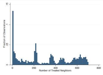
THE SOCIAL SIDE OF EARLY HUMAN CAPITAL FORMATION:
USING A FIELD EXPERIMENT TO ESTIMATE THE CAUSAL IMPACT OF NEIGHBORHOODS

                                           John A. List
                                         Fatemeh Momeni
                                           Yves Zenou

  This study was previously titled: Are Estimates of Early Education Programs Too Pessimistic?
  Evidence from a Large-Scale Field Experiment that Causally Measures Neighbor Effects. We
  thank Alec Brandon, Leonardo Bursztyn, Raj Chetty, Steven Durlauf, Nathaniel Hendren, Justin
  Holz, Michael Kremer, Thibaut Lamadon, Costas Meghir, Magne Mogstad, Julie Pernaudet,
  Stephen Raudenbush, Matthias Rodemeier, Juanna Schrøter Joensen, and Daniel Tannenbaum for
  valuable comments. We received helpful feedback from seminar participants at the University of
  Chicago, University of Wisconsin Milwaukee, Depaul University, Purdue University, and
  Monash University. We thank Clark Halliday, Uditi Karna, Alexandr Lenk, Ariel Listo, and Lina
  Ramirez for excellent research assistance.

  © 2020 by John A. List, Fatemeh Momeni, and Yves Zenou. All rights reserved. Short sections of
  text, not to exceed two paragraphs, may be quoted without explicit permission provided that full
  credit, including © notice, is given to the source.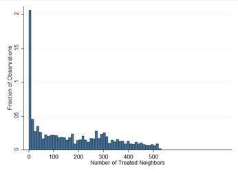
The Social Side of Early Human Capital Formation: Using a Field Experiment to Estimate
the Causal Impact of Neighborhoods
John A. List, Fatemeh Momeni, and Yves Zenou
December 2020
JEL No. C93,I21,I24,I26,I28,R1

                                          ABSTRACT

The behavioral revolution within economics has been largely driven by psychological insights,
with the sister sciences playing a lesser role. This study leverages insights from sociology to
explore the role of neighborhoods on human capital formation at an early age. We do so by
estimating the spillover effects from a large-scale early childhood intervention on the educational
attainment of over 2,000 disadvantaged children in the United States. We document large
spillover effects on both treatment and control children who live near treated children.
Interestingly, the spillover effects are localized, decreasing with the spatial distance to treated
neighbors. Perhaps our most novel insight is the underlying mechanisms at work: the spillover
effect on non-cognitive scores operate through the child's social network while parental
investment is an important channel through which cognitive spillover effects operate. Overall, our
results reveal the importance of public programs and neighborhoods on human capital formation
at an early age, highlighting that human capital accumulation is fundamentally a social activity.

John A. List                                     Yves Zenou
Department of Economics                          Department of Economics
University of Chicago                            Monash University
1126 East 59th                                   Caulfield VIC 3145
Chicago, IL 60637                                Australia
and NBER                                         yves.zenou@monash.edu
jlist@uchicago.edu

Fatemeh Momeni
Crime and Education Labs
University of Chicago
33 N LaSalle St.
Chicago, IL 60602
fmomeni@uchicago.edu
“... I will emphasize again and again: that human capital accumulation is a social activity, involving
groups of people in a way that has no counterpart in the accumulation of physical capital...” Lucas
(1988)

1    Introduction

Human capital theory can be traced to Mincer (1958), who created the framework to examine the
nature and causes of inequality in personal incomes. Empirically, human capital is typically opera-
tionalized as being measured in years of schooling completed and is commonly tied to labor market
outcomes. A key branch of this work explores individual’s educational investment decisions and
how those choices map into higher future incomes. A related line of work, estimating education pro-
duction functions, complements the human capital literature by investigating the determinants of
human capital (Heckman, 2008; Hanushek, 2020; Cotton et al., 2020). In this literature, standard-
ized test scores, or some other proxy for cognitive and executive function skills, are measured and
subsequently modeled as individual-specific skills potentially valued by employers. In this manner,
the received education production estimates reflect the long-run economic impacts of educational
inputs, effectively linking the two literatures (Hanushek, 2020).

To date, this line of economics research and related work in the contemporary psychology of educa-
tion literature are dominated by an empirical and theoretical focus on the individual (Schunk, 2020;
Cotton et al., 2020). This individual-centric approach has served the literatures well, as developing
knowledge on issues as varied as the foundations of learning to the causes and consequences of
human capital accumulation and skill formation, serve to deepen our understanding and clarify op-
timal policy solutions. Such insights also have frequently made their way into public policy circles,
either through advanced reforms or pedagogical changes in the classroom.

Yet, the Lucas’ quote in the epigraph summons a distinctly different line of inquiry, one which
includes the wisdom of Sociology to deepen our understanding of human capital accumulation.
As Jonassen (2004) notes, Sociology is concerned with many things, but primarily it relates to
explaining social phenomena, and this cannot be done if we examine individuals alone. Rather,
we must also scrutinize how people interact in group settings, and how those interactions shape
individuals and their choices, including those that augment human capital.

With this contribution in mind, our backdrop is that between 2010 and 2014, a series of early
childhood programs were delivered to low-income families with young children in the Chicago
Heights Early Childhood Center (CHECC; see Fryer et al., 2015; 2018). CHECC was located
in Chicago Heights, IL, a neighborhood on Chicago’s South Side with characteristics similar to
many other low-performing urban school districts. The goals of the intervention were to examine
how investing in cognitive and non-cognitive skills of low-income children aged 3 to 4 affects their

                                                  2
short- and long-term outcomes, and to evaluate the effectiveness of investing directly in the child’s
education versus indirectly through the parents. To that end, families of over 2,000 disadvantaged
children were randomized into (i) an incentivized parent-education program (Parent Academy),
(ii) a high-quality preschool program (Pre-K), or (iii) a control group. The children’s cognitive
and non-cognitive skills were assessed on a regular basis, starting before the randomization and
continuing into the middle and end of the programs. Follow-up assessments were also conducted
on a yearly basis.
Making use of these data, we consider insights from Sociology to focus on explorations of group
interactions. A useful starting point is Coleman (1988), who introduces social capital to parallel
economic concepts (physical capital and human capital) to embody relations among people. Once
in place, the effect of social capital is argued to have great import in the formation of human
capital, especially in the development of children. The Sociology literature has taken Coleman’s
work in several directions (Bourdieu, 1985; Putnam, 1993; Schuller, 2000), with critical factors of
early child human capital development relating to both parental relationships and the composition
of children’s peer play groups (Sheldon, 2002). Importantly, the Sociology literature teaches us
that detailing group composition at various ages of children is important since there are key age-
level interactions that affect human capital development of children (Cochran and Brassard, 1979;
Corsaro, 2005).
To explore the interplay between social interactions and human capital formation, we follow two
distinct steps. First, we provide causal evidence of the impact of neighborhood on educational
outcomes in early childhood. Instead of following the standard approach in economics, which uses
residential movers to identify neighborhood effects (see citations below), we exploit a unique form of
exogeneity induced by the CHECC intervention: the experimental variation in the spatial exposure
to treated families (within and between individuals) caused by the delivery of programs across
multiple years. By doing so, we are able to isolate the role of neighbors on individual outcomes and
examine how the exogenous changes in treated neighbors’ quality affect a child’s outcomes. Our
second step is to follow the Sociology literature to explore underlying mechanisms at work, both
from child to child as well as from parent to parent.
In the first step, we document large and significant spillover effects on both cognitive and non-
cognitive skills. We find the non-cognitive spillover effects are about two times larger than the
cognitive spillover effects. Our estimates suggest that, on average, each additional treated neighbor
residing within a three-kilometer radius of a child’s home increases that child’s cognitive score by
0.0033 to 0.0042 standard deviations (σ), whereas it increases her non-cognitive score by 0.0069σ
to 0.0070σ. Given that an average child in our sample has 178 treated neighbors residing within
a three-kilometer radius of her home—and making a (strong) assumption of linearity—we infer
that, on average, a child gains between 0.6σ to 0.7σ in cognitive test scores and about 1.2σ in non-
3cognitive test scores in spillover effects from her treated neighbors. As discussed more fully below,
the spillover effect is a key component of the total intervention effect. Interestingly, we find that
the spillover effects are localized and fall rapidly as the distance to a treated neighbor increases.
Fryer et al. (2015) also report interesting racial and gender heterogeneity in their treatment effects.
For example, through comparing outcomes between treatment and control children, they find the
Parent Academy significantly increases test scores for Hispanics and Whites, but does not improve
outcomes of Black children. These findings prompted us to examine whether such heterogeneities
also exist in our estimated spillovers. We find that non-cognitive spillover effects are significantly
larger for Blacks than Hispanics. According to our fixed-effects estimates, an additional treated
neighbor within a three-kilometer radius increases the non-cognitive test score of a Black child by
0.0100σ, whereas it increases the non-cognitive score of a Hispanic child by only 0.0045σ. We find
no significant racial differences in cognitive spillover effects. Focusing on gender, our estimates
suggest boys tend to benefit more than girls from cognitive and non-cognitive spillovers, although
these gender differences are not significant at the conventional levels. This observation is in the
spirit of previous empirical evidence on neighborhood effects, which tend to be larger for boys
(Entwisle et al., 1994; Halpern-Felsher et al., 1997; Leventhal and Brooks-Gunn, 2000; Katz et al.,
2001; Chetty and Hendren, 2018b).
Turning to Step 2, we recognize that the program effects from CHECC can spill over through
two main channels. The first channel is the direct social interactions between children who were
randomized during the intervention. Importantly, consonant with the Sociology literature, our
analysis includes observations from early childhood (3 to 4 years of age, when peer influence at
the neighborhood level starts) to middle childhood (8 to 9 years of age, when social interactions
within neighborhoods increase dramatically as children enter school). Therefore, direct exposure to
treated children who live in the same neighborhood is a likely mechanism that can generate spatial
spillover effects.1 The second channel is parental interactions. While Sociology presents a useful
guide, observational studies in the other sciences have also shown the import of this channel. For
example, Psychologists have found that neighborhoods can influence parental behavior and child-
rearing practices (Leventhal and Brooks-Gunn, 2000), which play critical roles in early development
(Cunha and Heckman, 2007; Waldfogel and Washbrook, 2011; Kautz et al., 2014; Fryer et al., 2015;
Kalil, 2015). Because CHECC also offered education programs to parents, treatment effects can spill
over through information and preference externalities, generated by parental social interactions.
To shed light on the mechanisms through which spillover effects operate, we start by comparing the
effects from neighbors who were assigned to the parental-education programs with the effects from
neighbors who were assigned to the preschool programs. Because, unlike in the Pre-K treatments,
1
See Epple and Romano (2011) and Sacerdote (2011) for recent reviews of the literature on peer effects in Eco-
nomics.
4the focus of Parent Academies was on educating parents rather than children, if spillover effects are
driven by interactions between parents, we might expect Parent Academy neighbors to generate
larger effects than Pre-K neighbors.2 Alternatively, larger spillovers from Pre-K neighbors than
from Parent Academy neighbors could imply the peer-influence channel plays an important role
in generating the effects. Our estimates suggest non-cognitive spillovers are more likely to operate
through preschool neighbors. According to our estimates, whereas an additional Parent Academy
neighbor within three kilometers of a child’s home induces a 0.0017σ to 0.0045σ increase in her
non-cognitive score, an additional Pre-K neighbor living within the same distance increases her
non-cognitive score by 0.0099σ to 0.0108σ. This finding suggests non-cognitive spillover effects are
more likely to operate through children’s rather than parents’ social networks. We do not find any
significant differences in cognitive spillover effects from Parent Academy and Pre-K neighbors.
Given our evidence suggesting peer influence at the neighborhood level is a key mechanism in gen-
erating non-cognitive spillover effects, we hypothesize that the racial differences in non-cognitive
spillovers might be at least partially driven by differences in social interactions within neighbor-
hoods. We explore this idea using data from the National Longitudinal Study of Adolescent Health
Survey. Our analysis confirms that African American adolescents are significantly more likely than
Hispanics to (i) know most people in their neighborhoods, (ii) stop on the street and talk to some-
one from the neighborhood, and (iii) use recreation facilities in the neighborhood. Although these
results cannot be interpreted as causal evidence, they are consistent with our previous finding that
social interactions with peers within neighborhoods is a key channel in generating non-cognitive
spillover effects.
Finally, our evidence suggests cognitive spillover effects are likely to operate—at least partially—
through influencing the parents’ decision to enroll their child in a (non-CHECC) preschool program.
Using survey data, we show that families with more treated neighbors are significantly more likely to
enroll their child in a preschool program (other than the ones offered at CHECC). Our evidence also
suggests children whose parents reported enrolling them in an alternative preschool program per-
form significantly better in cognitive assessments. Therefore, we conclude that influencing parental
investment decisions—as measured by the choice to enroll one’s child in a preschool program—is a
channel through which spillover effects on cognitive test scores operate.
We conclude our analysis by measuring the total impact of the intervention on children’s cognitive
and non-cognitive performance, accounting for the spillover effects. Our estimates suggest that,
on average, the intervention increased a treatment child’s cognitive (non-cognitive) test score by
0.82σ (1.32σ). Spillover effects make up a large portion of this total impact: whereas the average
direct effect of the intervention on a treatment child’s cognitive (non-cognitive) score is 0.11σ
2
This intuition does not rule out possible spillover effects from Pre-K neighbors that are generated through parental
interactions. After all, parents of children who received the Pre-K treatments might also be impacted through the
Pre-K programs. This intuition merely assumes Parent Academies affect parents more than Pre-K treatments do.
5(0.05σ), the corresponding indirect effect is 0.71σ (1.27σ). Control children also gain considerably
as a result of the intervention: on average, the intervention increased a control child’s cognitive
(non-cognitive) test score by 0.75σ (1.25σ). If we were to disregard the spillover effects on the
control group and had simply based our estimates of the total impact on the outcome differences
between the treatment and control children, we would have severely understated the total impact.
Specifically, this approach would have indicated that the intervention only improved the cognitive
(non-cognitive) test scores of a treatment child by 0.06σ (0.07σ). Ignoring spillover effects would
have also led us to underestimate the effects for African American children. Accounting for spillover
effects enables us to document a significant and large impact on non-cognitive performance that is
significantly larger for African Americans than Hispanics.
We view our results speaking to three distinct strands of research. First, we speak to the various
literatures that study the role of neighborhoods in shaping children’s short- and long-term human
capital outcomes. The empirical evidence on how neighborhoods affect children comes mainly
from observational studies that document correlations between neighborhood characteristics and
children’s outcomes, as well as studies that use experimental and quasi-experimental data to dis-
entangle the causal effects of neighborhood from selection effects.3 We contribute to this literature
in two important ways.
Our first contribution to this literature is to provide causal evidence on neighborhood effects by
exploiting a unique form of exogeneity, which was induced by our field experiment. The existing
experimental and quasi-experimental evidence on how neighborhoods shape children’s outcomes
identifies neighborhood effects using data from residential movers (e.g., Katz et al., 2001; Edin et
al., 2003; Kling et al., 2005; Åslund et al., 2010; Damm and Dustmann, 2014; Chetty et al., 2016;
Chyn, 2018; Chetty and Hendren, 2018a and 2018b). The identification of neighborhood effects
in this literature relies on instruments such as randomly assigned housing vouchers, quasi-random
assignment of immigrants to different neighborhoods, or public housing demolitions as sources of
exogenous changes in neighborhood quality. We take a different approach in that our identification
strategy leverages a field experiment that provides both within and between individual variation
in the spatial exposure to treated families.
Our second contribution to this literature is to provide insights on the role of neighbors in generating
neighborhood effects and the mechanism underlying these effects. Neighborhoods have multiple
attributes, which can each influence a child’s outcomes, such as school quality, crime rate, neighbors,
and so on. Unlike previous estimates on neighborhood effects, we are able to isolate and estimate
the effect of neighbors’ quality as one of the many channels through which neighborhoods can
influence children’s development. Specifically, our estimates suggest social interactions with other
3
See Leventhal and Brooks-Gunn (2000), Durlauf (2004), Ioannides and Topa (2010), Ioannides (2011), Topa and
Zenou (2015), Minh et al. (2017) and Graham (2018) for reviews of neighborhood effects on children.
6children in the neighborhood play an important role in the development of children’s non-cognitive
skills and that parental interactions influence a complementary aspect of child development.
The second strand of literature our study contributes to is the growing body of work that measures
spillover effects from programs and policy changes, designed to improve behaviors and outcomes in
various domains such as the labor market (Ferracci et al. 2014; Crépon et al., 2013; Lalive et al.,
2015; Muralidharan et al., 2017; Gautier et al., 2018), health (Miguel and Kremer 2004; Janssen,
2011; Avitabile, 2012), compliance behavior (Rincke and Traxler, 2011; Boning et al., 2018), voting
behavior (Sinclair et al., 2012; Gine and Mansuri, 2018), retirement saving decisions (Duflo and
Saez, 2003), and consumption (Angelucci and De Giorgi, 2009). We contribute to this literature by
providing the first evidence on spillover effects from a large-scale early education intervention, shed-
ding light on mechanisms, and estimating the total program impact when accounting for spillover
effects.
Finally, our results provide important insights for academics interested in modeling the formation
of early human capital, from economists to psychologists to sociologists. Within economics, for
example, a growing body of literature develops dynamic models of skill formation to explore the
role of various inputs in the production of cognitive and non-cognitive skills. Through structurally
estimating such models, this literature has found inputs such as schools, parental ability, home
environment, and parental investments to be important determinants in the formation of future
skills (e.g., Todd and Wolpin, 2007; Cunha and Heckman, 2007; Cunha et al., 2010; Attanasio et
al., 2015; Doepke and Zilibotti, 2017, 2019; Agostinelli et al., 2020; Attanasio et al., 2020; Boucher
et al., 2020; Cotton et al., 2020). We complement this literature by providing empirical evidence
for the role of neighbors’ influence at young ages. Our estimates suggest neighbors’ quality plays
an important role in producing cognitive and non-cognitive skills.
The remainder of the paper is structured as follows. Section 2 summarizes key features of our
intervention, randomization, and assessments. Section 3 describes our data and presents our es-
timation strategy. We present our main findings in section 4, where we report our estimates of
spillover effects on cognitive and non-cognitive test scores from a fixed-effects model, and explore
heterogeneities by race and gender. Section 5 presents our estimates of the spillover effects from a
lagged dependent variable (LDV) specification and discusses the robustness of our findings to using
this alternative identification strategy. We discuss the mechanisms in section 6. In section 7, we
estimate the total impacts of CHECC, break down these estimates into direct and indirect effects,
and discuss how ignoring indirect effects would bias our estimates. We discuss policy implications
and conclude in section 8.
72 Program Details
2.1 Overview of treatments
Between 2010 and 2014, a series of early childhood interventions were delivered to low-income
families with young children in Chicago Heights Early Childhood Center (CHECC). The center was
located in Chicago Heights, IL, which is a South Side, Chicago, neighborhood with characteristics
similar to many other low-performing urban school districts. According to the 2010 Census, black
and Hispanic minorities constituted about 80% of the population of Chicago Heights; its per-capita
income was $17,546 per year; and 90% of students attending the Chicago Heights School District
were receiving free or reduced-price lunches.
The main goals of this large-scale intervention were (i) to examine how investing in cognitive and
non-cognitive skills of low-income children 3 to 4 years of age affects their long-term outcomes,
and (ii) to evaluate the effectiveness of investing directly in children’s education versus indirectly
through their parents. To that end, families of over 2,000 children were randomized into either one
of four preschool programs (henceforth “Pre-K”) or one of the two parental-education programs
(henceforth “Parent Academy”) or a control group.
The Parent Academy was designed to teach parents to help their child with cognitive skills, such
as counting and spelling, as well as non-cognitive skills, such as working memory and self-control.
The curriculum for the Parent Academy was adapted from two effective preschool curricula: Tools
of the Mind, which focuses on fostering non-cognitive skills, and Literacy Express, which focuses
on improving cognitive skills.4 The curriculum was delivered to parents in eighteen, 90-minute
sessions, which were held every two weeks over a nine-month period. Parent Academy families
had the opportunity to earn up to $7,000 per year and could participate until their child entered
kindergarten. Earnings were based on parents’ attendance, their performance on homework, and
their child’s performance on the interim and end-of-year assessments. The two Parent Academy
treatments differed only in how they administered incentives. Payments made to families in the
“Cash” treatment were made via cash/direct deposits, whereas payments made to families in the
“College” treatment were deposited into an account that could only be accessed once the child was
enrolled in a full-time post-secondary institution.
Besides the Parent Academy, CHECC delivered four preschool programs in which children were
treated directly. We refer to these programs as Pre-K treatments. These four treatments dif-
fered in their curricula, as well as the duration and intensity of delivery. “Tools,” “Literacy,” and
“Preschool Plus” were nine-month full-day programs delivered during the school year, whereas
“Kinderprep” was a two-month half-day program delivered during the summer before a child en-
4
See Fryer et al. (2015) for more information on curriculum selection.
8tered kindergarten.5 The curriculum for “Tools” was Tools of the Mind, which focuses on improving
non-cognitive skills, whereas “Literacy” was based on Literacy Express,6 which focuses on foster-
ing cognitive skills.7 A new curriculum called “Cog-X” was developed for “Preschool Plus” and
“Kinderprep”, which emphasized both cognitive and non-cognitive skills.8
2.2 Randomization
Between 2010 and 2013, 2,185 children from low-income families in South Side, Chicago were
recruited and randomized into either one of the six treatments or the control group.9 The random-
ization took place once per year, at the beginning of each academic year.10 Some children were
randomized during more than one year, mainly to encourage families who were initially placed
in the control group to stay engaged with CHECC for assessments, by offering them a chance to
participate in future years.11 The yearly randomization schedule created four cohorts of children
we refer to by their year of randomization.12 Table 1 summarizes the randomization schedule for
each year of the program.
5
Preschool Plus and Kinderprep also offered a parental component that was much less extensive than the Parent
Academies, both in terms of education time and incentives. Parent Academy parents could earn up to $7,000 based on
their attendance, their performance on homework, and their child’s performance on assessments, whereas Preschool
Plus and Kinderprep parents could only earn up to $900 and $200, based merely on their attendance to parental
workshops. Preschool Plus and Kinderprep treatments also offered fewer instruction time to parents. Whereas Parent
Academy parents could spend 27 hours in parental workshop, Preschool Plus and Kinderprep parents were offered
a maximum of 21 and 6 hours of parental education, respectively. The intensity of the preschool component of
Preschool Plus was similar to that of “Tools” and “Literacy Express” in terms of instruction time.
6
For more information on Literacy Express see http://ies.ed.gov/ncee/wwc/interventionreport.aspx?sid=
288.
7
For more information on Tools of the Mind see http://toolsofthemind.org.
8
Fryer et al. (2020) evaluated “CogX” under the assumption that the programs did not affect the outcomes of the
control group. Through comparing the performance of treatment and control children, the authors found “Cog-X”
treatments significantly improved cognitive scores (by about one quarter of a standard deviation), but failed to find
any significant effects on non-cognitive scores. For more information on Pre-K programs, see Fryer et al. (2020).
9
See Appendix A for maps of residential addresses.
10
The exceptions were years three and four of the intervention during which randomization took place twice per
year: In the first randomizations, children were randomized into either the nine-month preschool program, the
summer Kinderprep program, or the control group; and in the second, a smaller group of families were recruited and
randomized into either the summer kindergarten preparation program or the control group. Table 1 combines the
two randomizations.
11
As a result, some children who were in the control group in an earlier year were randomized into a treatment
group in later randomizations. In a few cases, a child who was randomized into a treatment group in an earlier year
was assigned to a different (or the same) treatment in later randomizations. Overall, 1,675 children were randomized
only once, 509 were randomized twice, and one child was randomized in three years.
12
Those children who were randomized in multiple years also appear in multiple cohorts.
9Table 1: Randomization by Year
Parent 9-Month Kindergarten
Control
Academies Pre-K Preparation
Cohort-1
242 153 172 0
(2010)
Cohort-2
443 216 166 0
(2011)
Cohort-3
422 0 196 107
(2012)
Cohort-4
376 0 104 99
(2013)
Unique child 1270 317 539 206
Notes: The number of children randomized into each treat-
ment group in each year of the intervention is reported. The
bottom row presents the number of unique children in each
group, over the course of four years.
2.3 Assessments
Our key outcome measures are children’s performances in cognitive and non-cognitive assessments,
which were used to evaluate the programs. These assessments consist of a pre-assessment admin-
istered to all incoming students prior to randomization, a mid-assessment between January and
February, a post-assessment, which occurred in May, immediately after the school year ended, and
a summer assessment at the end of the summer. Besides the assessments that took place during the
program year, graduated children were also assessed annually every April, starting the year after
they finished the program. These assessments are referred to as age-out assessments. Appendix B
presents the assessment schedule for all four cohorts.
Assessments included both cognitive and non-cognitive components and were administered by a
team of trained assessors. The cognitive component used a series of nationally normed tests,
measuring general intellectual ability and specific cognitive abilities such as receptive vocabulary,
verbal ability, oral language, and academic achievements. The non-cognitive component included a
combination of subtests measuring executive functions such as working memory, inhibitory control,
and attention shifting, as well as a questionnaire completed by assessors, which measured self-
regulation in emotional, attentional, and behavioral domains.
3 Data and the Econometric Model
Before describing our empirical approach at a detailed level, we find it potentially useful to provide
a roadmap for our exploration. Overall, we identify the spillover effects from CHECC by exploiting
10certain unique features of our data. First, conditional on the total number of neighbors who signed
up to participate, the number of neighbors who were subsequently assigned to treatment is deter-
mined exogenously through the randomization process. We leverage this experimental variation in
spatial exposure to treatments across children to estimate spillover effects. Second, our main iden-
tification strategy also exploits the panel nature of our data and the within-individual variation in
exposure to treated neighbors induced by delivery of programs over multiple years. Specifically, by
including individual-specific fixed effects, our estimates control for any time-invariant individual,
family, and neighborhood unobserved characteristics that might be correlated with spatial expo-
sure to treatments. We also estimate the effects under a second model that relaxes the assumption
of time-invariant omitted variables by controlling for the lagged dependent variables (LDV) and
dispensing with the fixed effects (Section 5). Whereas our main identification strategy uses within-
individual variations to estimate the spillover effects, the LDV specification estimates the effects
by exploiting both within-individual and between-individual variations in spatial exposure to treat-
ments. Our findings, presented below, are robust to using this alternative specification.
3.1 Data
3.1.1 Construction of outcome variables
Our outcome measures are indices generated from standardized test scores on cognitive and non-
cognitive assessments.13 The cognitive assessment included the Peabody Picture Vocabulary Test
(PPVT), which assesses verbal ability and receptive vocabulary (Dunn et al., 1965), and four
subtests of the Woodcock Johnson III Test of Achievement (WJ): (i) WJ-Letter and Word Identi-
fication (WJL), which measures the ability to identify letters and words; (ii) WJ-Spelling (WJS),
which measures the ability to correctly write orally presented words; (iii) WJ-Applied Problems
(WJA), which measures the ability to analyze and solve math problems; and (iv) WJ-Quantitative
Concepts (WJQ), which assesses the knowledge of mathematical concepts, symbols, and vocabulary
(Woodcock, McGrew and Mather, 2001).
The non-cognitive component included the Blair and Willoughby Executive Function test (Willoughby,
Wirth and Blair, 2012), which is composed of three subtests assessing attention (Spatial Conflict),
working memory (Operation Span), and attention shifting (Same Game) and the Preschool Self-
Regulation Assessment (PSRA), which is designed to assess self-regulation in emotional, attentional,
and behavioral domains (Smith-Donald et al., 2007).14
13
These indices were constructed by Fryer et al. (2015, 2020) for the original evaluations of the programs.
14
Because Blair and Willoughby tests are designed for preschool, a new test was added for assessments that were
administered to older children (age-out assessments). For children in kindergarten or older, the Same Game test of
Blair and Willoughby was replaced with a variant of Wisconsin Card Sort game, which measures attention shifting
for children of that age. For more information, see www.parinc.com/Products?pkey=478.
11A cognitive index was made up of averaged percentile scores on each cognitive subtest, and a non-
cognitive index was made up of average percent-correct scores on each non-cognitive subtest. The
two indexes were then standardized by the type of assessment (pre-assessment, mid-assessment,
etc.), including the entire study population (treated and control) who took that assessment, to
obtain a zero mean and standard deviation of one.
To explore the spatial spillovers on both treatment and control children, we construct three samples:
a pooled sample, including observations from both treatment and control groups; a control sample,
including data from control children; and a treatment sample, including observations from treated
children. Our treatment sample pools observations from children who were randomized into any of
the programs. We include observations from the baseline to the fourth age-out assessment. Our final
control, treatment, and pooled samples include 2,442, 3,074, and 5,208 observations, respectively.15
Appendix C presents the details regarding how we construct these three samples.
Table 2 provides summary statistics on the baseline demographic variables for our pooled sample.
Note the majority (90%) of the children are either African American or Hispanic, and 53% live in
families with an annual household income under $35,000.
3.1.2 Addresses and neighbor counts
To estimate the spatial spillover effects from the intervention, we follow the literature (see, e.g.,
Miguel and Kremer, 2004 and subsequent work) and calculate the number of treated neighbors of
a child at a given time and use it as a measure of spatial exposure to treatments. To do so, we
start by calculating commuting distances between the home locations of all pairs of children who
were randomized during the intervention.16 Commuting distances are calculated by considering the
street network structure and its restrictions (e.g., one-way roads, U-turns, etc.) and finding the
closest driving distance between each pair. The average travel distance between a pair of children
in our sample is 8.52 kilometers (std. dev.= 8.07), and 99.8% of the sample resides within 60
kilometers of each other. Figure 1 presents a histogram of travel distances between home locations
of all children who were randomized during the intervention.
We define a pair as neighbors if the commuting distance between the two is less than “r” kilometers,
and we call “r” the neighborhood radius. We conduct our analysis for various values of neighborhood
treated ) and control (N control ) neighbors of each
radii. We then calculate the number of treated (Ni,t|r i,t|r
child i at the time of her assessment t, and define the total number of CHECC neighbors of i as
15
Note that the number of observations in the pooled sample is smaller than the sum of the number of observations
in our control and treatment samples. The reason is that in a few cases, when a child was first randomized into
the control group and was placed into a treatment group in later randomizations, the pooled sample only includes
observations that took place after the child was randomized into treatments. See Appendix C for more information.
16
Distances were calculated using the ArcGIS OD Cost Matrix Analysis tool.
12Table 2: Baseline Summary Statistics for the Pooled Sample
Variable Share/Mean Variable Share/Mean
Gender Mother’s Education
Male .51 Less than high school .08
Race Some high school but no diploma .12
Black .40 High school diploma .13
Hispanic .50 Some college but no degree .17
White .09 College degree .18
Other Race .01 Other .06
Missing Race .01 Missing Mother’s Education .25
HH Income and Unemployment Benefits Father’s Education
below 35K .53 Less than high school .09
36K-75K .14 Some high school but no diploma .1
75K+ .06 High school diploma .13
Missing Income .26 Some college but no degree .12
Receives Unemployment Benefit .09 College degree .08
Missing Unemployment Benefit .31 Other .06
Missing Father’s Education .44
45.32
Baseline Age (months)
(6.91)
Notes: Summary statistics for baseline demographic variables are presented. For education lev-
els, Some high school but not diploma includes parents with a GED or high school attendance
without a diploma, College degree includes associate’s, bachelor’s and master’s degrees, Less than
high school includes an education level below 9th grade or no formal schooling, and Other in-
cludes vocational/technical or other unclassified programs. Standard deviations are reported in
parentheses.
total = N treated + N control . Note that as more children are randomized into treatment and control
Ni,t|r i,t|r i,t|r
groups over the four years of the intervention, the number of treated and control neighbors vary
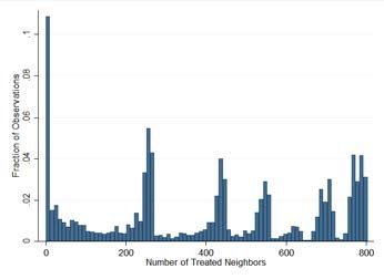
over time.17 Table 3 reports the summary statistics for Ni,t|r
treated and N control , and Figure 2 presents
i,t|r
treated , for various values of neighborhood radii. Whereas
histograms of the exposure measure Ni,t|r
treated is small, as the neighborhood radius increases to 3
for r = 1 kilometers, the variation in Ni,t|r
kilometers and beyond, we gain considerable variations in the exposure measure.
3.2 Econometric model
We exploit three unique features of our data to estimate the spillover effects. First, conditional on
total ), the number of
the total number of a child’s CHECC neighbors at a given point in time (Ni,t|r
treated ) is determined exogenously through the
neighbors who are randomized into treatments (Ni,t|r
intervention. Second, the repeated assessment schedule generates a panel, which enables us to track
performance over time. Finally, multiple randomizations and the delivery of programs over the four
17
Because more children were receiving the treatments over the four-year span of the intervention, and a neighbor
who was previously in the control group in an earlier randomization might be assigned into a treatment group in
control treated
later years, Ni,t|r can both increase or decrease over time. However, Ni,t|r can only increase over time, because
no child who was already treated could be assigned into the control group in later years.
13Figure 1: Histogram of distances between children in the study. The horizontal axis is cut at 30
kilometers.
treated .
years of the intervention create within-individual variations in our exposure measure Ni,t|r
Although the experimentally induced variation in our exposure measure serves as an important
feature, which we exploit for identification, our estimation strategy does not rely on it exclusively.
Given our limited sample size and the fact that the intervention was not designed to measure
spatial spillovers, our exposure measure could be correlated with individual- or neighborhood-level
unobservable characteristics. Therefore, we exploit the panel nature of our data to provide clean
estimates of the spillover effects. The above three properties allow us to estimate the spillover
treated ) through a fixed-effects
effects using within-individual variations in our exposure measure (Ni,t|r
specification. This technique uses the variations in spatial exposure over time and controls for any
unobserved time-invariant individual-, family-, or neighborhood-level characteristics that might be
treated .
correlated with Ni,t|r
We estimate spatial spillover effects from CHECC, using an individual fixed-effects specification of
the form:
treated total
Yi,t = β0 + β1 Ni,t|r + β2 Ni,t|r + γi + δt + i,t , (1)
treated
where Yi,t is the standardized cognitive or non-cognitive test score of a child i on test t, Ni,t|r
total represents
represents the number of treated neighbors of i at time t as previously defined, and Ni,t|r
the total number of i’s neighbors who were randomized in the intervention by time t.18 γi and δt
18
As aforementioned, Miguel and Kremer (2004), Giné and Mansouri (2018) and Bobba and Gignoux (2019) use
similar specifications to estimate spatial spillover effects. Similar to our specification, these studies use the number
of treated individuals within a certain neighborhood radius as their measure of spatial exposure to treatments,
and control for the total number of neighbors in their regression analyses. Distinct from these studies, which rely
exclusively on the experimentally induced variations in the distribution of treated neighbors across individuals, we
14Table 3: Neighbor Counts by Neighborhood Radius
r= 1 km r = 3 km r = 5 km r = 7 km
27.89 178.13 325.63 422.81
Nrtreated
(27.73) (154.21) (238.75) (272.08)
29.49 183.47 333.73 437.79
Nrcontrol
(31.84) (165.34) (257.95) (301.11)
Notes: This table presents the average number of treated and
control neighbors of a child in our pooled sample, for various
definitions of neighborhood radii. The numbers reflect all the
observations in our pooled sample for which we observe both
cognitive and non-cognitive scores. Standard deviations are re-
ported in parentheses.
are individual and test (time) fixed effects. Under this specification, β1 represents the average
effect of moving one of the control neighbors of a child i to a treatment group, holding the total
number of her CHECC neighbors constant. This measure (β1 ) provides an intuitive estimate on the
spillover effects from the intervention because it enables a policymaker to weigh the benefits against
the costs associated with treating an additional child in the neighborhood. Section 5 presents an
alternative model, which relaxes the assumption of time invariance for individual effects and exploits
both within-individual and between-individual variation in spatial exposure to treated neighbors to
estimate spillover effects. As we will further discuss in Section 5, our findings are robust to using
this alternative specification.19
4 Results
4.1 Main findings
We estimate spillover effects for the neighborhood radii of 3, 5, and 7 kilometers. As Figure 2
treated becomes too small,
suggests, when neighborhood is defined too narrowly, the variation in Ni,t|r
limiting our power to estimate the effects. Therefore, we start with a neighborhood radii of 3
treated to estimate the effects.
kilometers and larger, which provides us with enough variation in Ni,t|r
Arguably, these choices of neighborhood radii are economically relevant. According to the National
Household Travel Survey, the average commuting distance to school for a 6 to 12 year-old child
are able to exploit the panel nature of our data and identify the spillover effects using within-individual variations
in exposure to treatments and remove all unobserved time-invariant individual-level characteristics that might be
correlated with the spatial exposure to treatments.
19
As a robustness check, we also run the regressions without baseline observations and our effects remain similar.
15(a) r=1 km (b) r=3 km
(c) r=5 km (d) r=7 km
treated for r = {1, 3, 5, 7} kilometers.
Figure 2: Histogram of Ni,t|r
is about 6 kilometers (3.6 miles).20 The average travel time from home to work for a Chicago
Heights resident is estimated to be 26.1 minutes (US Census Bureau statistics), which translates
to about 21 kilometers for a speed of 30 miles per hour.21 Because schools and workplaces provide
natural interaction spaces for children and their parents, we can reasonably assume our choices of
neighborhood radii are relevant distances within which social interactions can generate spillovers.
Table 4 presents estimated β1 ’s from equation (1) for neighborhood radii of 3, 5, and 7 kilometers.
Standard errors—clustered at the census-block-group level to allow for common error components
within geographical units—are reported in parentheses below each point estimate. The left (right)
panel presents the average spillover effect from treating an additional neighbor of a child on her
standardized cognitive (non-cognitive) test score. Columns (1) and (4) report the pooled effects
on both treatment and control children and reveal significant positive spillover effects on both
cognitive and non-cognitive test scores. The effects on non-cognitive scores are more than double
the effects on cognitive scores: an additional treated neighbor within 3 kilometers of a child’s home
20
https://nhts.ornl.gov/briefs/Travel%20To%20School.pdf
21
This estimate is consistent with a report by the National Household Travel Survey that suggests the av-
erage commuting distance from home to work in the US is about 19 kilometers (11.8 miles). For more
information, see: https://www.bts.gov/sites/bts.dot.gov/files/docs/browse-statistical-products-and-data/national-
transportation-statistics/220806/ntsentire2018q1.pdf (page 73).
16increases her cognitive score by 0.0033σ (p < 0.01), whereas it increases her non-cognitive score by
0.0069σ (p < 0.01). Empirical differences in cognitive and non-cognitive spillovers are statistically
significant.22
Columns (2) and (3) parse the effects on cognitive scores by treatment assignment. These estimates
reveal that both treatment and control children benefit from living close to treated families. While
the control group benefits slightly more than the treatment group from cognitive spillover effects, the
difference is not significant at conventional levels.23 Columns (5) and (6) report the spillover effects
in non-cognitive scores by treatment assignment. These estimates illustrate that the treatment
and control children both benefit from non-cognitive spillovers. The estimated spillover effects on
non-cognitive scores on the control and treatment groups are very similar and are not significantly
different across the two groups.24 These findings are robust to the choice of neighborhood radius,
r.25,26
In sum, we document significant positive spillover effects on both cognitive and non-cognitive test
scores and find the effect sizes are significantly larger for non-cognitive scores versus cognitive
scores.27 Yet, the richness of the data permits us to explore deeper into both the nature and extent
of such spillovers.
4.2 Spatial fade-out
A closer examination of the estimated β1 ’s reported in Table 4 suggests an important spatial
pattern: the spillover effect from an additional treated neighbor becomes smaller as we broaden the
neighborhood radius from 3 to 7 kilometers. To further explore this pattern and shed light on the
relationship between spillover effects and distance, we provide Figure 3, which shows the estimated
β1 ’s for a broader range of r’s.28 Note that the effects on both cognitive and non-cognitive scores
operate very locally.
As we increase the neighborhood radius, the marginal spillover effects from an additional treated
22
The p-values from the Wald test of the null hypothesis H0: β1cog = β1ncog against H1: β1cog 6= β1ncog are 0.001,
0.03, and 0.06 for neighborhood radii of 3, 5, and 7 kilometers, respectively.
23
The p-values from the Wald test of equal β1cog ’s for the control and treatment group are 0.11, 0.16, and 0.13 for
neighborhood radii of 3, 5, and 7 kilometers, respectively.
24
The p-values from the Wald test of equal β1ncog for treatment and control group for neighborhood radii of 3K,
5K, and 7K meters are 0.80, 0.84, and 0.78.
25
Appendix E breaks down these effects by subtests and explores which components of the cognitive/non-cognitive
index generate the effects.
26
Appendix D discusses the robustness of our estimated spillover effects to the exclusion of individual fixed effects
from our main specification and to the exclusion of other controls and lagged dependent variables from our alternative
(LDV) specification.
27
In Appendix F, we explore the potential role of sorting by estimating the effects using a subsample of children who
attended the majority of assessments. Our evidence suggests that selection is not an important factor in generating
our results.
28
The point estimates are reported in Appendix G.
17Table 4: Mean Effect Sizes on Cognitive and Non-cognitive Scores, Fixed-Effects Estimates
Cognitive Scores Non-cognitive Scores
Pooled Control Treatment Pooled Control Treatment
(1) (2) (3) (4) (5) (6)
0.0033*** 0.0038*** 0.0016 0.0078*** 0.0069*** 0.0064***
r = 3 km
(0.0010) (0.001) (0.0010) (0.0013) (0.0015) (0.0013)
0.0021*** 0.0023** 0.0010* 0.0043*** 0.0037*** 0.0034***
r = 5 km
(0.0006) (0.0008) (0.0006) (0.0008) (0.0011) (0.0008)
0.0018*** 0.0021*** 0.0008* 0.0033*** 0.0025*** 0.0028***
r = 7 km
(0.0005) (0.0007) (0.0005) (0.0007) (0.0010) (0.0007)
Obs. 5,208 2,442 3,074 5,208 2,442 3,074
Notes: Spillover effects from each additional treated neighbor (βˆ1 ) estimated from
equation (1) are presented. Columns 1-3 (4-6) represent the average spillover
effects from an additional treated neighbor on a child’s standardized cognitive
(non-cognitive) score. Robust standard errors, clustered at the census-block-group
level, are in parentheses; *** pPooled
Control Treated
Figure 3: The spillover effect from having an additional treated neighbor on a child’s standardized
cognitive and non-cognitive scores, as functions of neighborhood radius.
did not induce externalities to the control group. They found that the assignment to Parent
Academies increases a child’s non-cognitive scores by 0.203σ, but does not significantly impact
cognitive scores. Moreover, the authors reported positive treatment effects on cognitive and non-
cognitive scores for Hispanic children, but did not find any significant treatment effects on African
American children. Parent Academy was also reported to have slightly larger effects on girls than
boys, although the gender differences were not significant. Motivated by the heterogeneity in
treatment effects from the Parent Academy component of the intervention reported in Fryer et
al. (2015), we investigate whether children of different races (or gender) benefit differently from
spillover effects. We do so by estimating equation (1), separately by race and gender.
Since African American and Hispanic children make up over 90% of our sample, our analysis
on heterogeneity along race focuses on these two groups. Panel (a) of Table 5 and Figure 4
presents βˆ1 ’s separately for African American and Hispanic children. Comparing the effects across
races, we find no significant differences in cognitive spillover effects between Hispanics and African
19Americans. In contrast to the effects on cognitive scores, however, spillovers on non-cognitive scores
are significantly larger for African Americans than Hispanics.30 The empirical estimates indicate
that, on average, an additional treated neighbor increases the non-cognitive scores of an African
American child by about two to three times more than a Hispanic child. For instance, an additional
treated neighbor within a 3-kilometer radius increases the non-cognitive score of a Hispanic child
by 0.0045σ, whereas it increases an African American child’s non-cognitive score by 0.0100σ.
Table 5: Mean Effect Sizes within Gender and Race Subgroups, Fixed-Effects Estimates
(a) Race (b) Gender
Cognitive Scores Non-cognitive Scores Cognitive Scores Non-cognitive Scores
(1) (2) (3) (4)
African American Boys
0.0014 0.0100*** 0.0048*** 0.0088***
r = 3 km
(0.0015) (0.0024) (0.0016) (0.0019)
0.0007 0.0055*** 0.0029*** 0.0048***
r = 5 km
(0.0008) (0.0015) (0.0009) (0.0012)
0.0009 0.0042*** 0.0024*** 0.0038***
r = 7 km
(0.0008) (0.0012) (0.0007) (0.0010)
Obs. 2,087 2,087 2,583 2,583
Hispanic Girls
0.0042*** 0.0045*** 0.0017 0.0068***
r = 3 km
(0.0013) (0.0014) (0.0011) (0.0019)
0.0027*** 0.0019** 0.0013* 0.0037***
r = 5 km
(0.0009) (0.0008) (0.0007) (0.0011)
0.0023*** 0.0016** 0.0011 0.0028***
r = 7 km
(0.0007) (0.0008) (0.0006) (0.0009)
Obs. 2,580 2,580 2,625 2,625
Notes: The spillover effects from each additional treated neighbor on cognitive and non-cognitive test scores, estimated from
the fixed-effects model (equation (1)). Panel (a) presents the effects, separately for African American and Hispanic receiving
children. Panel (b) reports the effects separately for boys and girls. Robust standard errors, clustered at the
census-block-group level, are in parentheses; *** preported by Fryer et al. (2015) due to two main differences between our samples. First, unlike
Fryer et al. (2015) who report heterogeneous effects from the Parent Academy, our analysis uses
data from all CHECC programs and considers heterogeneity in spillover effects on all children who
were randomized during the intervention. Second, whereas Fryer et al. (2015) base their estimates
on observations from the post program assessments (which took place immediately after the end
of program year), our estimates use the pre-, mid-, and post-program assessment as well as up to
four additional follow-up assessments, which were administered after a program year ended.
(a) Race (b) Gender
Figure 4: The spillover effect from an additional treated neighbor on a child’s standardized cognitive
and non-cognitive scores, estimated from the fixed-effects model. Panel (a) presents the effects
separately for African American and Hispanic children, and panel (b) presents the effects separately
for males and females.
5 Robustness
Our identification strategy, presented in Section 3 (individual fixed-effects model), is based on the
assumption that individual effects are time-invariant omitted variables. In this section, we relax
this assumption by directly controlling for the lagged dependent variables and removing individual
fixed effects. Whereas the fixed-effects specification uses within-individual variations in spatial
exposure to treatments, the lagged dependent variables (LDV) model exploits both within- and
between-individual variations to estimate the spillover effects.
In this spirit, Angrist and Pischke (2008) argue that fixed effects and LDV estimates have a brack-
eting property such that they provide upper and lower bounds for where the true effect lies. The
authors provide an empirical approach to estimate the effects under both specifications and check
21You can also read