IS LARGE-SCALE RAPID COV-2 TESTING A SUBSTITUTE FOR LOCKDOWNS?
←
→
Page content transcription
If your browser does not render page correctly, please read the page content below
Is large-scale rapid CoV-2 testing a substitute for lockdowns?
               Marc Diederichs1 , René Glawion2 , Peter G. Kremsner3,4 , Timo Mitze5
               Gernot J. Müller3,6,7 , Dominik Papies3 , Felix Schulz1 , Klaus Wälde1,6,8∗
(1)
      Johannes Gutenberg University Mainz, (2) University of Hamburg, (3) University of Tübingen
               (4)
                   Centre de Recherches Médicales de Lambaréné, Lambaréné, Gabon
                   (5)
                       University of Southern Denmark, (6) CESifo, (7) CEPR, (8) IZA

                                             August 3, 2021

          BACKGROUND: Various forms of contact restrictions have been adopted in re-
          sponse to the Covid-19 pandemic. Around February 2021, rapid testing appeared
          as a new policy instrument. Some claim it may serve as a substitute for contact
          restrictions.
          OBJECTIVES/METHODS: We evaluate the effects of a unique policy experiment:
          In March and April 2021, the city of Tübingen set up a testing scheme while relaxing
          contact restrictions. We compare case rates in Tübingen county to an appropriately
          identified control unit.
          CONCLUSIONS: The experiment led to an increase in the reported case rate. This
          increase is robust across alternative statistical specifications. An epidemiological
          model that corrects for ’more cases due to more testing’ and ’reduced testing and
          reporting during the Easter holiday’ also confirms the finding.

    Can large-scale CoV-2 testing strategies substitute for restrictive public health measures?
In theory, the idea is straightforward. If, first, every socially active person is subjected to a
rapid CoV-2 test on a regular basis and, second, quarantined if tested positive, there is (almost)
zero infection risk from social interactions. One would achieve the same outcome as under a
complete lockdown—albeit at much lower costs: social interactions could be maintained.
    In practice, there are several complications. Any testing procedure generates false negatives,
that is, some infections will necessarily go undetected (1 ). Moreover, the timing of testing is
critical: when testing takes place too early, infected persons go undetected, when it takes place
too late, the transmission of the disease may have already taken place. Some therefore suggest
that rapid tests do more harm than good (2 ). Lastly, testing and quarantining may be not
sufficiently comprehensive, for instance, because of a lack of compliance.
    Lockdowns, on the other hand, are also unlikely to prevent new infections altogether. First
and foremost, they cannot be complete because some social interactions are essential. Second,
their effectiveness also suffers from lack of compliance (3 , 4 ).
    Given this debate, an empirical assessment seems warranted. This paper turns to a uniquely
suited policy experiment set up in the German town of Tübingen. Between March 16 and April
24, 2021, it ran a large-scale rapid testing scheme while simultaneously relaxing lockdown
      ∗
     Contact details of authors: Marc Diederichs, Felix Schulz and Klaus Wälde (corresponding author), Jo-
hannes Gutenberg University Mainz, Gutenberg School of Management and Economics, Jakob-Welder-Weg
4, 55131 Mainz, Germany, fax + 49.6131.39-23827, phone + 49.6131.39-20143, e-mail waelde@uni-mainz.de;
René Glawion, University of Hamburg, Faculty of Business, Economics and Social Sciences, Von-Melle-Park 5,
20146 Hamburg; Peter G. Kremsner, Institute of Tropical Medicine, University of Tübingen, Tübingen, Ger-
many, Centre de Recherches Médicales de Lambaréné, Lambaréné, Gabon; Timo Mitze, University of South-
ern Denmark, Faculty of Business and Social Sciences, Department for Border Region Studies Alsion 2, 6400
Sønderborg/Denmark; Gernot Müller and Dominik Papies, Universität Tübingen, Nauklerstr. 50, 72074 Tübin-
gen, Germany.

                                                     1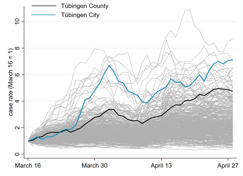
measures (appendix A.1). Each negatively-tested person was permitted, inter alia, to shop,
go to movie theaters or join other people in restaurants (outdoors). While several towns tried
to obtain similar permits elsewhere in Germany (5 ), the case of Tübingen is unique as its
experiment started while other German counties were still in lockdown. We rely on these
counties as a reference group in our synthetic control method (6 –9 ) to assess whether large-
scale rapid CoV-2 testing can be a substitute for lockdowns. The answer would be yes if opening
under safety did not increase cases in Tübingen.

1     Findings
1.1    Empirical findings
We describe the pandemic state by the key metric for policy decisions in Germany: the seven-
day SARS-CoV-2 case rate (appendix A.2.1). The left panel in figure 1 shows the development of
the case rate between February and April 2021. The solid black line in the left panel represents
the development in Tübingen county, the dashed red vertical lines indicate the start and end
of the policy experiment. The line for Tübingen county shows that the case rate was below 50
before the start of the project and increased to almost 150 during the Easter weekend starting
April 2. This increase coincided with opening under safety (OuS) and led to wide public claims
that “Tübingen failed”.

                Figure 1: Seven-day case rates of Tübingen and control group

    Statistics tells us, however, that we cannot assess the causal effect of a policy experiment by
comparing the case rate before and after the start of the project. Other factors than OuS are
likely to have affected pandemic dynamics in Tübingen over this period as well. We, therefore,
need to compare the pandemic development in Tübingen county to a control group of similar
counties: counties should display comparable pandemic dynamics before the start of OuS in
Tübingen, should share certain fundamental socio-demographic and health care characteristics
(e.g., population density, age structure, medical services, commuting patterns) and should be
subject to very similar if not identical public health measures.
    We identify such a set of control counties using the synthetic control method (see section 2).
The resulting control counties and their weights constituting our synthetic control county are

                                                2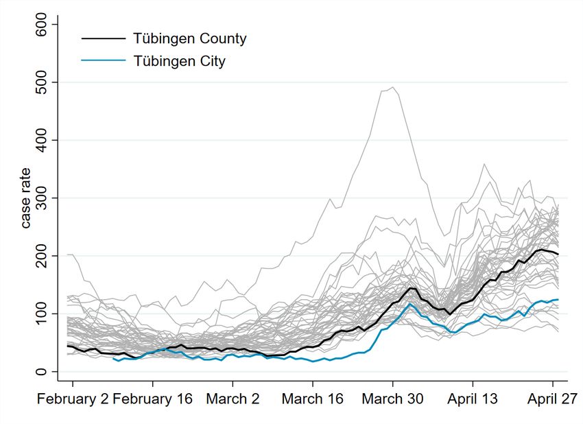
presented in table 1. The synthetic control county consists of four urban districts (’Stadtkreis,
SK’) and four rural districts (’Landkreis, LK’). Two of the three units that receive the largest
weights (Freiburg and Heidelberg) are cities in Baden-Württemberg with major universities
that have similar population levels of up to 230K and comparable socio-demographic structures.
Local health care systems are also similar. Table 5 in the appendix shows the details of the fit.

                    Table 1: Control counties and their weights for figure 1
           name                   weight             name                    weight
           SK Freiburg i.Breisgau  0.29              LK Pfaffenhofen a.d.Ilm  0.07
           LK Eichstätt           0.24              LK Bitburg-Prüm         0.05
           SK Heidelberg           0.19              SK Münster              0.04
           SK Oldenburg            0.09              LK Lüneburg             0.03

    Given this background, we can now again turn to figure 1. The solid black line, representing
Tübingen county, and the grey line, representing the synthetic control, show very similar case
rates prior to the beginning of the experiment, indicating a good fit in the pre-treatment
period since February 2021. When we compare the development in reported case rates after
the beginning of the experiment, we initially observe a parallel development between Tübingen
county and its synthetic twin. At the beginning of April, cases in the control county start to
decline, whereas the decline in Tübingen county only sets in a few days later. By April 10, the
gap between Tübingen county and the control county is almost closed.
    This development is also visible in the right panel of figure 1. A first peak in the difference
between treatment and control occurs 2.5 weeks after the start around April 3, just around
the Easter weekend. The right panel also shows that this difference, while visible, is hardly
statistically different from zero at the 10% level. Nevertheless, a treatment effect is visible:
OuS seems to increase the case rate – at least temporarily.
    As of April 10, however, data not included in our earlier version (10 ), case rates in Tübingen
more strongly increase relative to its synthetic twin. While some open questions related to OuS
in Tübingen will be addressed in our discussion section, the most straightforward interpretation
of this increase after April 10 is the continuation of a process OuS initiated on March 16: More
contacts lead to more cases. The reduction in the gap between Tübingen and its synthetic
twin is due to the Easter holidays and the slowdown of reporting of data from laboratories and
doctors to local and national health authorities.

1.2     Testing and the Easter break
Any empirical finding calls for a theoretical interpretation. Empirically, we find that OuS
increases case rates. Theoretically, at least two questions arise: Did case rates increase only
because OuS implies more testing and when we test more, we find more? Second, can we believe
our verbal interpretation that OuS and the Easter break imply such a non-monotonic behavior
as visible in figure 1? We answer these questions in turn.

1.2.1   Case rates and testing
Some argue that the number of reported infections increases when there is more testing. The
argument is not convincing when a test is undertaken because a patient with Covid-19 symptoms
visits a doctor. If doctors arrange for tests, the number of tests depends on the number of
patients with Covid-19 symptoms. The number of reported infections therefore increases only
when there are more patients with symptoms. Tests increase as a function of the state of the
pandemic (11 ).

                                                 3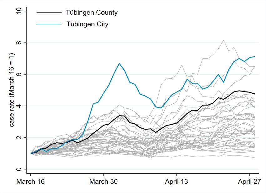
The argument is true when testing is the outcome of projects such as OuS. In this case, the
number of tests does not depend on the state of the pandemic but on the number of participants
that want to be tested. Similar arguments can be made with respect to testing travelers, testing
sport professionals, or all other preventive testings. In this case, more infected individuals are
found when there is more testing.
    To understand the quantitative importance of this argument for OuS, we extend a standard
SIR model in four respects (appendix A.5.2). We (a) allow for rapid testing leading to (b)
discovery of asymptomatic (unreported) cases who, thereby, (c) turn into reported cases. We
assume that (d) reported infectious individuals are in quarantine and infections can only occur
when meeting a non-reported infectious individual (12 ). OuS in this framework consists of
these four features plus an increase in the contact rate, i.e., as an example, the number of
individuals one person meets per day.
    When we want to separate the effect of more contacts from the effect of more testing, we
first fit the extended SIR model to the data (appendix A.5.2). Second, we switch off the testing
channel by assuming that no extra testing takes place: in this case, the model predicts that, all
else equal, the increase in (reported) cases is less strong initially (appendix A.4.2). This finding
supports the notion that more testing leads to more (reported) cases. However, the effect is
quantitatively small (with a maximum of 7%) and vanishes over time because the increase in
case rates accelerates in the absence of testing (and quarantining). Hence, the fact that more
testing leads to more cases is unlikely to be the reason for the strong increase in the case rate
in Tübingen (figure 1) in the context of OuS.

1.2.2    OuS and Easter break
Our complete explanation of figure 1 builds on a combination of a (i) permanent OuS effect
and a (ii) temporary Easter break effect. OuS has a permanent effect on the contact rate,
the Easter break temporarily reduces reporting and testing. We capture these two effects by
an additional feature of our SIR model (appendix A.5.2) that lets the flow from exposed to
reported infectious individuals fall over Easter. A certain share of infectious individuals who
display symptoms do not go to an emergency center and therefore do not get tested.
    Employing this framework shows that one can easily explain the rise in case rates in Tübin-
gen by an increase in contact rates (appendix A.4.3). The temporary drop over the Easter
break can be understood by a reduction in transmission and testing. This finding holds when
we estimate one unique increase of contacts and when we estimate two separate contact rates,
one before and one as of Easter (table 6). We concede that the Easter effect in the SIR model
is not as pronounced as in the data. What we can clearly see, however, is that the permanent
effect of OuS can easily explain the entire increase in case rates. Our theoretical interpretation
therefore confirms our empirical findings. OuS did increase case rates in Tübingen relative to
its control group.

2       Method
    • Implementing the synthetic control method

    We estimate the causal effect of OuS (the ‘treatment’) on infection dynamics in Tübingen
(the ‘treated unit’) by relying on the synthetic control method (SCM). It was proposed for the
causal assessment of policy interventions based on aggregate outcome measures (6 , 7 ). At the
heart of this method lies an estimator which identifies, in our application, counties in Germany
to which Tübingen county can be compared (the ’synthetic control county’). This comparison
is based on information observable prior to treatment and summarized by a set of predictor

                                                 4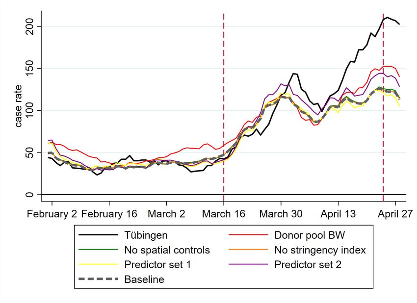
variables (the ’predictor set’). SCM requires an a-priori list of counties (the ’donor pool’) from
which to construct the control unit. See appendix A.5.1 and table 5 for more background.
    Results depend on how we measure the pandemic (the ’outcome variable’). Our preferred
outcome variable is the 7-day case rate. We also employ cumulative cases and, briefly, the
positive rate, as alternatives. Robustness checks for the predictor set, the donor pool and
outcome variables are undertaken and will be discussed shortly.
    The present study puts special emphasis on two novel predictor variables. First, we allow
for spatial controls. They are due to the low case rate of Tübingen compared to other counties
in Germany before the start of OuS on March 16, visible in figure 4. If visitors enter Tübingen
from counties with higher case rates, Tübingen will likely experience higher case rates itself. To
this end, we looked for control counties that were also surrounded by counties with case rates
similar to the neighbors of Tübingen. If Tübingen is subject to a ’catching up’ process, we
wanted to make sure that Tübingen is compared with regions that are also subject to ’catching
up’.
    Second, it appears very important that counties are as similar as possible to Tübingen
county in terms of Covid-19 policies. We achieved this goal in two ways. On the one hand, we
constructed an index (see appendix A.2.4) that measures the stringency of Covid-19 policies.
As an alternative, we compare Tübingen to counties from its state Baden-Württemberg only.
Counties all coming from the same state as Tübingen are very homogeneous with respect to
their Covid-19 rules.

    • Estimating an extended SIR model

The differential effects of ’opening’ and of ’safety’ (i.e. testing) in OuS can be understood and
quantified by estimating an extended SIR model (13 –15 ). Our central extension of a standard
SIR model (appendix A.5.2) consists in modeling rapid testing and the Easter break.
    Testing implies a flow from asymptomatic, non-reported individuals to reported individuals.
Assuming that all reported individuals enter quarantine, the share of infectious individuals in
society (one can meet) falls due to testing. The Easter break implies that (i) test results are
not reported to health authorities and that (ii) not all individuals with symptoms visit doctors.
    We quantify the parameters of both extensions by matching cumulative cases, case rates
and observed positive tests. We do so by minimizing the squared difference between data and
model predictions (14 ). We infer the effects of testing on the reported number of infections
by computing a hypothetical time series for cases under the assumption that no testing was
undertaken in Tübingen. The effect of the Easter break is quantified by estimating the share
of individuals that do not visit emergency units despite having symptoms.

3     Discussion
Findings from a comparison of a county with a synthetic county depend on (a) the measure
used (outcome variable), (b) the criteria employed to find comparable counties (predictor set)
and (c) the group of counties from which to choose comparable counties (donor pool). Varying
our choices confirms the basic finding.

3.1    Predictor sets and donor pool
The outcome of our main robustness checks for Tübingen county are visible in figure 2. In
addition to our predictor set ’baseline’, employed for estimating results displayed in figure 1, we
structure our discussion around two additional predictor sets, a predictor set 1 and a predictor
set 2. Our baseline predictor set, visible in table 5, was discussed in the method section.

                                                5
Predictor sets 1 and 2 (visible in tables 14 and 16, respectively) shorten the pre-treatment
period, starting on February 1 in the baseline predictor set, to a start date of March 1. This
investigates into the importance of pandemic pre-treatment variables for the pre-treatment fit
and for the overall result. Predictor set 1 employs daily case rates while predictor set 2 employs
weekly case rates. Predictor set 2 therefore further reduces the importance of pre-treatment
pandemic measures relative to non-pandemic variables. To understand the importance of spatial
controls and of the stringency index, we employ a predictor set defined as the baseline predictor
set without the stringency index and another one defined as baseline without spatial controls.

         Figure 2: Seven-day case rates for alternative predictor sets and donor pools

    As figure 2 shows, all of our robustness analyses confirm the baseline scenario. This is
most impressively visible by the hardly visible (grey dashed) baseline graph in this figure: the
predictor set without the stringency index leads to basically the same result. When we take
out spatial controls, the prediction gets slightly better. This means that the ’catching up’
argument laid out in the method section does not have a large quantitative importance. The
shorter pre-treatment fitting period of predictor set 1 leads to a somewhat worse prediction
than baseline. Again, quantitatively, this is of no importance.
    Going from daily to weekly pre-treatment frequency with predictor set 2 worsens the pre-
treatment fit but improves the post-treatment prediction. The same is true when we restrict the
donor pool to Baden-Württemberg only. If we therefore put more emphasis on homogeneity in
Covid-19 policy, we could tell a somewhat more optimistic story. Given the worse pre-treatment
fit (RMSPE of 19.57 in table 10 instead of 9.9 in table 5), however, we do not put too much
emphasis on this finding. We conclude that our baseline result is confirmed by these robustness
tests that vary the predictor set and the donor pool.

3.2    The role of the pandemic measure
The seven-day case rate as employed in figure 1 is the measure of the pandemic state that
receives most of the attention around the world. It is not clear, however, whether this is the

                                                6
best measure for a pandemic. It is also not clear whether this is the best measure to compare
the evolution of the pandemic across regions. A moving average over a period of seven days
is much more short-run in nature than, for example, the sum of all new infections since some
starting point.
We therefore employ the total number of reported infections since January 2021 per 100,000
inhabitants as dependent variable. Appendix A.7 shows that the synthetic twin of Tübingen
consists of different counties than in our benchmark analysis. The fit dominates the baseline
fit as cumulative infections over a longer period than only seven days are less volatile. Finding
similar counties is therefore easier for the SCM. What is most important, however, is the
evaluation of OuS: We confirm the findings from above. Interestingly, Tübingen and its control
also move more or less in parallel up to around April 1. Only then, the difference becomes
much larger, just as in the case of the case rates.
An alternative popular measure of the severity of a pandemic is the positive rate, i.e. the
share of positive tests in the total number of tests being undertaken in a certain population.
This was the official measure of the scientific team behind OuS in Tübingen (of which one of us
was the head) and of policy-makers. By this measure, there was no increase in the severity of
the pandemic in Tübingen. Local outbreaks in communities and residential homes might have
increased the case rate in the county but were not visible in the positive rate.
3.3 Is Tübingen city different?
Many commentators on OuS in Tübingen have argued that conclusions drawn from Tübingen
county could be misleading. One should rather study Tübingen city. Probably findings on OuS
would be less negative in this case, the claim goes.
The details of the timing of OuS in Tübingen are in table 2. All testing and opening measures
took place in the city of Tübingen. As of April 6, only shopping in non-essential stores for local
residents continued. Those parts of the experiments that attracted most visitors had ended.
Maybe the increase in case rates in Tübingen county is due to increases in communities other
than Tübingen city (see figure 17 for a map).
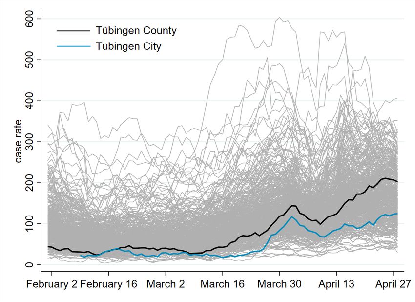
To study this hypothesis, we first look at the evolution of case rates in Tübingen city, also
shown in figure 4 in addition to Tübingen county. We observe that Tübingen city had indeed an
(even) lower level of case rates than Tübingen county. We also see that Tübingen city followed
the same overall trend as Tübingen county. What is more, figure 5 shows that increase in case
rates in Tübingen city is larger than the increase in Tübingen county. This raises some doubts
about the hypothesis.
To be on the safe side, we treat Tübingen city as an independent county and apply the SCM
again. We adjust the predictor set (as different data are available at the community level than
at the county level), the donor pool and the pandemic measure (see appendix A.9). We also
adjust the pandemic measure as Tübingen city had one of the lowest, if not the lowest, case
rates in all of Germany before the treatment date. This makes it impossible to construct an
appropriate synthetic twin employing the case rate as pandemic measure. The new pandemic
measure we use for Tübingen city is therefore the growth factor for case rates.
Before proceeding, we confirm that the use of a new predictor set and a new pandemic
measure do not strongly affect our findings: We compare our baseline findings with findings
based on the new predictor set and the new pandemic measure. Applying SCM then finally
to Tübingen city shows that Tübingen city experienced a stronger increase in (growth of) case
rates than its control regions.
Returning to the hypothesis, it is true that the increase in case rates in other communities
belonging to Tübingen county contributed to the rise of cases in Tübingen county. There is
just as much truth to the finding, however, that Tübingen city experienced a rise in case rates
7as well and that this rise is larger than the increase in comparable control counties.
Acknowledgments
We would like to thank Peter Martus for guidance to testing data, Boris Palmer for support
with data on Tübingen city and Oliver Piehl for general data support and background on
official reporting of CoV-2 infections. For this research project, authors are solely funded by
their universities, contributed equally and declare no competing interests.
References
1. J. Dinnes et al., en, Cochrane Database of Systematic Reviews, Publisher: John Wiley &
Sons, Ltd, issn: 1465-1858, (2021; https://www.cochranelibrary.com/cdsr/doi/10.
1002/14651858.CD013705.pub2/full) (2021).
2. G. Guglielmi, “Rapid coronavirus tests: a guide for the perplexed”, Nature, news feature.
3. G. Graffigna et al., PLoS ONE 15(9): e0238613. (2020).
4. N. B. Masters et al., PLoS ONE 15(9): e0239025, https://doi.org/10.1371/journal.pone.0239025
(2020).
5. M. Diederichs, T. Mitze, F. Schulz, K. Wälde, https://www.macro.economics.uni-mainz.de/klaus-
waelde/ongoing-work-and-publications/, (https://www.macro.economics.uni-mainz.
de/files/2021/05/Evaluation_Augustusburg-Zwischenbericht-final.pdf) (2021).
6. A. Abadie, A. Diamond, J. Hainmueller, SYNTH: Stata module to implement Synthetic
Control Methods for Comparative Case Studies, Statistical Software Components, Boston
College Department of Economics, Oct. 2011, (https : / / ideas . repec . org / c / boc /
bocode/s457334.html).
7. A. Abadie, A. Diamond, J. Hainmueller, American Journal of Political Science 59, 495–
510 (Apr. 2015).
8. T. Mitze, R. Kosfeld, J. Rode, K. Wälde, Proceedings of the National Academy of Sciences
117, 32293–32301, issn: 0027-8424, (https://www.pnas.org/content/117/51/32293)
(2020).
9. B. Born, A. M. Dietrich, G. J. Müller, PLOS ONE 16, 1–13, (https://doi.org/10.
1371/journal.pone.0249732) (Apr. 2021).
10. M. Diederichs et al., medRxiv, eprint: https://www.medrxiv.org/content/early/2021/
04/26/2021.04.26.21256094.full.pdf, (https://www.medrxiv.org/content/early/
2021/04/26/2021.04.26.21256094) (2021).
11. K. Wälde, IZA DP No. 13785, http://ftp.iza.org/dp13785.pdf (2020).
12. T. C. Jones et al., Science, eprint: https://science.sciencemag.org/content/early/
2021/05/24/science.abi5273.full.pdf (2021).
13. W. O. Kermack, A. G. McKendrick, Procceedings of the Royal Society 115, 700–721
(1927).
14. J. R. Donsimoni, R. Glawion, B. Plachter, K. Wälde, German Economic Review 21, 181–
216 (2020).
15. J. Dehning et al., Science 369 (2020).
8A Supplementary appendix
Is large-scale rapid CoV-2 testing a substitute for lockdowns?
Marc Diederichs1 , René Glawion2 , Peter G. Kremsner3,4 , Timo Mitze5
Gernot J. Müller3,6,7 , Dominik Papies3 , Felix Schulz1 , Klaus Wälde1,6,8†
(1)
Johannes Gutenberg University Mainz, (2) University of Hamburg, (3) University of Tübingen
(4)
Centre de Recherches Médicales de Lambaréné, Lambaréné, Gabon
(5)
University of Southern Denmark, (6) CESifo, (7) CEPR, (8) IZA
August 3, 2021
†
Contact details of authors: Marc Diederichs, Felix Schulz and Klaus Wälde (corresponding author), Jo-
hannes Gutenberg University Mainz, Gutenberg School of Management and Economics, Jakob-Welder-Weg
4, 55131 Mainz, Germany, fax + 49.6131.39-23827, phone + 49.6131.39-20143, e-mail waelde@uni-mainz.de;
René Glawion, University of Hamburg, Faculty of Business, Economics and Social Sciences, Von-Melle-Park 5,
20146 Hamburg; Peter G. Kremsner, Institute of Tropical Medicine, University of Tübingen, Tübingen, Ger-
many, Centre de Recherches Médicales de Lambaréné, Lambaréné, Gabon; Timo Mitze, University of South-
ern Denmark, Faculty of Business and Social Sciences, Department for Border Region Studies Alsion 2, 6400
Sønderborg/Denmark; Gernot Müller and Dominik Papies, Universität Tübingen, Nauklerstr. 50, 72074 Tübin-
gen, Germany.
A-1A.1 The experiment
In order to appreciate the experiment under study, consider the developments in Germany
prior to this experiment. German policy measures in response to the Corona pandemic are
set at the state level. While policies differed somewhat across the 16 German states, all states
agreed to a range of measures in response to the second wave in December 2020. In particular,
non-essential shops, restaurants, and schools were closed. These measures were partly reversed
in early March 2021 against the backdrop of rising infections numbers, presumably because the
second wave of infections had died off by late February.
Tübingen is located in the state of Baden-Württemberg (BW, for short). Here, non-essential
shops were opened on 8 March 2021, provided that the case rate in the county was below 50.
Otherwise, a ‘click & meet’ scheme was put in place (i.e., shopping was permitted for customers
with appointment). Teaching at primary schools resumed on March 15. These measures were
announced on March 5 by the state government and hence implemented on short notice.
Table 2: Time of policy experiment
Date Change in permitted activities
March 16, 2021 Opening of nonessential shops, outdoor dining, theaters, cin-
emas, etc. in Tübingen city center; official negative rapid test
(”day ticket”) required
March 27, 2021 Number of day tickets for visitors from outside Tübingen
county limited to 3,000 per day
April 1, 2021 Day tickets no longer available to visitors from outside Tübin-
gen county
April 6, 2021 Outdoor dining no longer possible
April 24, 2021 Experiments ends
While regulations in Tübingen were mostly the same until then, the state government
announced on March 15 that starting the next day (see table 2), the town of Tübingen would
embark on a special experiment, centered around a large-scale rapid testing scheme, officially
labeled ‘Opening under Safety’ (‘Öffnen mit Sicherheit’). The town set up 9 testing posts
where everybody could be tested with a rapid antigen test free of charge. The capacity for
daily testing was 9000 and there were more than 30K tests per week (1 ). 15 minutes after the
test, the result would be released and in case it was negative, the subject was provided with
a ‘day ticket’ entitling the holder to shop in non-essential stores, attend bars and restaurants
(outdoors), cinemas and theaters (the OuS activities). In case the test was positive, people
were asked to take a PCR test. A positive PCR test result is automatically reported to the
public health office (‘Gesundheitsamt’). The PCR tests form the basis for the official statistics
on which our analysis is based. OuS ended on Saturday, 24 April, due to a change in the
‘Bundesinfektionsschutzgesetz’ adopted by the German federal parliament.
Below the level of the 16 states, Germany is subdivided into a total of 401 counties (“Land-
kreise” and “kreisfreie Städte”). Tübingen city (pop: 91K) is part of Tübingen county (pop:
229K). In total, there are 44 counties in BW. The experiment under study took place in Tübin-
gen city only. Still, everyone living in Tübingen county was allowed to participate. Hence,
spillovers from the city to other areas of the county may have potentially been significant. Our
main analysis therefore focuses on a comparison of Tübingen county to other counties. Also,
detailed data is available only at the county level.
To measure the causal impact of OuS, it is important to note that Tübingen is not ex-
ceptional in terms of fundamentals. However, it performed relatively well compared to its BW
peers regarding CoV-2 case numbers (see appendix A.6.2 for more background). At some point,
A-2Tübingen county was indeed enjoying the lowest case rate in all of BW. Still, there have been
many counties which did similarly well during the period. The experiment taking place in
Tübingen rather than elsewhere is most likely due to local idiosyncrasies and politics that are
orthogonal to infection dynamics. The experiment, while approved by the state government,
was devised jointly by the town’s major and the Corona commissioner of Tübingen county.
Both have gained prominence in national media as a result of vocal and eloquent interventions
regarding the handling of the pandemic and, more importantly, because of their personalities.
It seems that these personalities, rather than any special developments in Tübingen, have been
causal for setting up the Tübingen experiment. It thus comes close to a randomized control
trial.
A.2 Data
A.2.1 General information
• Cases, cumulative cases and case rates
To avoid confusion, it is useful to remind us of definitions of (cumulative) cases and case
rates. The number of SARS-CoV-2 cases reported on a day t is given by the number of new
infections on day t − 1. Cumulative cases over the previous d days on day t is given by the sum
of cases from t − 1 − d to t − 1. The seven day case rate on day t is given by cumulative cases
over the previous 7 days relative to t, divided by population size and multiplied by 100K.
• County-level data
Data on reported SARS-CoV-2 infections at the county level are taken from the Robert
Koch Institute (2 ). Infections are identified by PCR tests. For our empirical analysis, we use
aggregate case numbers for each county and day based on the reporting date by local health
authorities. Time-varying predictors are the average daily temperature and daily mobility
changes for each county during the pre-treatment period until March 16, 2021. Mobility changes
(in percent) based on individual mobile phone data are computed as the difference in mobility
patterns between a specific date and the average value for the corresponding weekday from the
same month in 2019 (pre-COVID benchmark period). To give a specific example: The mobility
change for Wednesday, March 10, 2021, is calculated as the difference in the number of regional
trips for this date and the average number of trips on Wednesdays in March 2019. We use data
on daily temperatures from Deutscher Wetterdienst (3 ), and updated data on mobility changes
per county and day are obtained from (4 ).
We further include time-constant cross-sectional predictors characterizing regional demo-
graphic structures and the regional health care system as in (5 ) based on data from the INKAR
online database of the Federal Institute for Research on Building, Urban Affairs and Spatial De-
velopment (6 ). We use the latest year available in the database, which is 2017, and rely on the
following cross-sectional predictor variables: population density (population/km2 ), the share of
females in the population (in %), the average age of female and male population (in years), old-
and young-age dependency ratios (in %), the number of medical doctors per 10,000 of popula-
tion and pharmacies per 100,000 of population, the regional settlement structure (categorical
dummy), and the share of highly educated population (in %).
A-3• Community-level data
To supplement our county-level-analyses with an analysis at the city level, we obtained daily
case rates for the city of Tübingen for the treatment period directly from the city’s Corona
Commissioner. For the pre-treatment period, we rely on weekly case rates that were provided
to us by the local health authorities (https://www.kreis-tuebingen.de/17094149.html).
• SCM data and repository
Data used for our SCM-based analysis fall into four groups: Data for our main county
analysis, for the Tübingen city analysis, for the stringency index (section A.2.4) and some
rapid test data (displayed in figure 3).
All of these data plus the corresponding Stata, R and matlab scripts are available in a public
repository at https://figshare.com/s/87f712ecb2f9eaf044b1.
A.2.2 Descriptive statistics
Table 3 shows descriptive statistics for variables we employ for our main analysis. The variables
are measured at the county level and the underlying population is Germany without direct
neighboring counties of Tübingen (which are Böblingen, Esslingen, Reutlingen, Zollernalb,
Freudenstadt and Calw). The latter are excluded from all analyses. Panel A contains all
variables related to measuring the development of the pandemic. Panel B displays information
on the time-varying predictors, mobility and average air temperature, and panel C shows all
predictors related to the county’s demographic structure and their health care coverage.
Table 3: Descriptive statistics
Mean S.D. Min. Max.
A: Data on reported CoV-2 cases
Seven-day CoV-2 case notification rate per 100,000 116.53 72.60 3.74 663.76
Cumulative infections per 100,000 inhabitants since January 1st 6290.96 8803.45 387 164461
Cumulative cases over previous 7 days 232.10 309.93 2 7340
Cumulative cases over previous 14 days 448.63 589.31 7 13428
Neighbourhood (50km) seven-day case rate per 100k 116.01 58.55 0 552.48
B: Time-varying predictors
Average mobility -.10 .13 -.69 .73
Average temperature 3.70 4.81 -17.5 19
Stringency index 2.88 .18 2.38 3.16
C: Regional demographic structure and local health care system
Population density (inhabitants/km2 ) 535.44 705.39 36.13 4686.17
Share of females in population (in %) 50.60 .64 48.39 52.74
Average age of female population (in years) 45.88 2.12 40.70 52.12
Average age of male population (in years) 43.18 1.84 38.80 48.20
Old-age dependency ratio (persons aged 65 years
34.39 5.49 22.40 53.98
and above per 100 of population aged 15-64 years)
Young-age dependency ratio (persons aged 14 years
20.53 1.44 15.08 24.68
and under per 100 of population aged 15-64 years)
Medical doctors per 10,000 of population 14.62 4.42 7.33 30.48
Pharmacies per 100,000 population 27.04 4.91 18.15 51.68
Categorical variable$ for population density of NUTS3 region 2.60 1.05 1 4
Share of highly educated* persons in regional population (in %) 13.05 6.21 5.59 42.93
Notes: * = International Standard Classification of Education (ISCED) Level 6 and above; $ = included categories are 1) larger
cities (kreisfreie Großstädte), 2) urban districts (städtische Kreise), 3) rural districts (ländliche Kreise mit Verdichtungsansätzen),
4) sparsely populated rural districts (dünn besiedelte ländliche Kreise).
A-4A day-by-day overview of the number of tests and positive cases is provided in figure 3.
On April 1, participation in the experiment was restricted to inhabitants of Tübingen county.
Accordingly, we find a structural break in the data on this date with around twice as many
tests being administered before (on average 2888 per day) than after the restriction (1373 daily
tests). We are able to differentiate the number of positive tests into participants from Tübingen
city, Tübingen county and elsewhere. We point out that the number of positive tests taken
by visitors from the county after April 1 can be explained by commuting staff that was also
frequently tested.
Figure 3: Total number of tests (left) and positive tests by origin of tested individual (right)
8000
6000
10
positive tests
all tests
City
4000
County
5 Visitors
2000
0 0
Apr 01 Apr 15 May 01 Apr 01 Apr 15 May 01
A.2.3 Tübingen and its donor pool
The SCM selects control counties from a donor pool. When we compare Tübingen to all regions
in the donor pool, we get a first idea about the trend of Tübingen relative to other counties and
about the highest and the lowest possible treatment effect. Figure 4 plots case rates of Tübingen
county and Tübingen city within case rates of all German counties in the left panel. The right
panel shows the same two time series within case rates of all counties from Baden-Württemberg.
Figure 4: Seven-day case rates in Germany (left) and Baden-Württemberg (right)
Judging the effect of OuS from these figures is difficult for many reasons. One reason is
that treated and control regions start from different levels. Figure 5 therefore normalizes the
case rate on the treatment date (16 March) in all counties to 1. One can then directly read
from the resulting figure whether the growth process in the treated regions was stronger over
the treatment period than in control regions.
While these figures, of course, also do not allow to draw any causal conclusions about OuS,
the relative increase of Tübingen city to Tübingen county came as a surprise. While Tübingen
A-5city always has a lower incidence (level), its incidence growth is much more pronounced, both
relative to Tübingen county and relative to all counties in Baden-Württemberg.
Figure 5: Normalized seven-day case rates in Germany (left) and Baden-Württemberg (right)
A.2.4 A stringency index for German states and counties
Understanding the effects of almost anything related to the pandemic requires a detailed un-
derstanding of the institutional environment. Any region is subject to a long list of regulations
that govern contacts in the private, in the public and on the workspace. In our analysis, we
account for the largely decentralized policy framework enacted by German states and counties.
Ideally, our synthetic control region consists of counties with a regime similar to pre-OuS con-
ditions in Tübingen. To this end, we construct an index of the stringency of health regulations,
similar to previous efforts based on an ordinal classification of measurements (7 , 8 ). Building
on the Infas database (9 ) and prior experience in this field of research (10 ), we are able to
observe differences across counties.
The available data allows us to distinguish between k = 1...K domains like e.g. kinder-
gartens, shops and restaurants. Up to 16 distinct policies are documented for each domain. In
line with the other indices, we group the policies by strictness into five levels from 0 to 4. Hence,
for each region i, day t and domain k, there is a vector Li,t,k with 16 values. The highest of
these 16 values is given by max Li,t,k . The index Ii,t ∈ [0, 4] is then calculated as daily averages
of the maximum value of the K = 23 domains,
K
1 X
Ii,t = max Li,t,k . (A.1)
K k=1
A first impression of the stringency of policies over time is given in figure 6. We plot the index I
on the vertical and time on the horizontal axis. Each of the German states is represented using
an individual color, Tübingen county is highlighted as the black line. As the figure reveals,
policies are very homogeneous across counties. While there are 401 counties in Germany, there
are rarely more than 20 different values visible at any point in time.
For our SCM, we include the index in the pre-treatment period in the predictor set. This
provides us with a control group that enforced measurements of similar scope and severity prior
to the experiment as Tübingen did. We cannot use the index, however, to detect other OuS
projects across Germany. This is due to the focus of the Infas database on county legislature.
OuS projects are in most cases restricted to single communities and in many cases not mentioned
in the county legislature. This makes it impossible to point out relevant regions based on the
index. We therefore proceed with an exclusion of counties based on our compilation of OuS
projects across Germany in table 4. The source for this search is general public information.
We make sure that none of these counties appears in any of our synthetic control counties.
A-6Figure 6: Stringency index across all 401 German counties.
3
2
1
0
Apr 2020 Jul 2020 Oct 2020 Jan 2021
Table 4: Opening under Safety projects in Germany as of April 23, 2021
Community County Start End Source
Tübingen (City) Tübingen March 16 April 23* tuebingen.de
Weimar (City) Weimar (City) March 29 March 31 tmasgff.de
Augustusburg Mittelsachsen April 1 April 23* augustusburg.de
Nordhausen Nordhausen April 6 April 16 mdr.de
Alsfeld Vogelsbergkreis April 8 April 15 alsfeld.de
several Harz April 9 April 23* kreis-hz.de
Baunatal Kassel April 12 April 23* baunatal.de
several Schleswig-Flensburg April 19 ongoing ostseefjordschlei.de
several Rendsburg-Eckernförde April 19 ongoing ostseefjordschlei.de
all counties in the state of Saarland April 6 April 23* saarland.de
Note: All end dates marked with a * have ended due to the enactment of unitary federal restrictions on April 24 (11 )
A.3 Literature
There have been calls for comprehensive and large-scale testing schemes early in the pandemic
(12 ). In theory, it is clear that testing and quarantining can dramatically reduce the costs of
an epidemic (13 ). A systematic empirical assessment, however, of the benefits of widespread
rapid testing based on antigen tests is still missing (14 ). In the present paper, we contribute to
such an assessment by studying a unique policy experiment in which widespread rapid antigen
tests were coupled with opening of non-essential infrastructure. We estimate the causal effect
of this intervention using the synthetic control method (15 –17 ). This method, SCM for short,
is the vehicle for our empirical identification strategy.
SCM has been frequently used in the social sciences to study the effect of policy interven-
tions, broadly defined, on political, social, and economic outcomes (17 ). In these contexts,
SCM has been shown to be a flexible and robust estimation tool. In addition, it has also
been applied to COVID-related research, for instance, to study the effectiveness of lockdown
measures by means of a counterfactual analysis for Sweden (18 , 19 ) and to study the effect
of shelter-in-place policies in California (20 ). (10 ) use SCM to study the effect of face masks
A-7on SAR-CoV-2 cases in Germany. The SCM approach was also used in the interim evaluation
of the Liverpool mass-scale testing project (21 ). Similar to the Tübingen experiment, this
pilot was centered around repeated testing of asymptomatic individuals. Those with a negative
result were not allowed, however, to participate in otherwise restricted activities. Compared to
the synthetic control region, they find that large scale testing does not significantly decrease
case numbers and hospitalization. In a different context, SCM allowed quantifying the impact
of the Brexit referendum on economic performance in the UK (22 ).
A.4 Findings
A.4.1 Our baseline result
The synthetic twin county employed in figure 1 consists of control counties who are listed,
jointly with their weights, in the main text in table 1. Table 5 below displays the criteria
(predictors) which serve as basis for constructing the synthetic twin. Predictor values pertain
to the pre-treatment period ending March 16, 2021.
Predictors can be split into groups: lagged pandemic measures (the outcome variable) and
structural regional characteristics, which are expected to influence the local infection dynamics
over time. As the table shows, we place a strong emphasize on lagged values of the seven-day
case rate as predictor in order to ensure that Tübingen and the selected control regions follow
a common pre-trend in the last two weeks before the OuS experiment stated in Tübingen. We
also include an average measure for the cumulative number of SARS-CoV-2 cases in the two
weeks before treatment start.
It would have been nice to include data on (UK) mutant shares. Unfortunately, they are not
available at the county level. We (implicitly) capture mutant effect by focusing on pre-treatment
pandemic dynamics when selecting control regions.
With regard to structural regional characteristics, we use both time-varying and time-
constant predictors. As such, we use average levels for daily temperature and intra-regional
mobility changes in the week prior to the treatment. The link between seasonality and infec-
tion dynamics has recently been studied (23 ). Including mobility effectively controls for social
interaction as a driver of local infection dynamics and also as a measure how closely people
follow prevailing (lockdown) policy rules (24 ).
Additionally, we control for the share of females in population, average age of female popu-
lation, average age of male population, old-age dependency ratio, young-age dependency ratio,
medical doctors per population, pharmacies per population, categorial variable for population
density of counties and share of highly educated persons in regional population as suggested in
(5 ). The rationale behind the inclusion of these predictors is to match Tübingen as closely as
possible to its synthetic control group in terms of socio-demographic factors and factors related
to the local health care system. Previous research has shown that these factors are significantly
related to differences in COVID-19 incidence and death rates at the sub-national level (25 ).
The fit of the weighted predictor variables of the control counties from table 1 with respect
to corresponding variables in Tübingen can be seen from comparing column 2 and 3 in table
5. Overall, there is a good fit. The population density is roughly twice as high in the synthetic
control group as in Tübingen. We do not believe, however, that this is crucial for our findings. If
anything, our effects are underestimated as the speed at which infection spread should be higher
in more densely populated counties. The overall good fit underlines the good pre-treatment fit
between the seven-day case rate development in Tübingen and its synthetic control group, as
already visualized in figure 1.
A-8Table 5: Balancing properties of predictor set ’baseline’ for figure 1
Treated Synthetic
Seven-day case rate per 100k (Feb 1) 44.30 49.48
Seven-day case rate per 100k (Feb 8) 31.45 34.44
Seven-day case rate per 100k (Feb 15) 31.89 32.19
Seven-day case rate per 100k (Feb 22) 40.31 32.70
Seven-day case rate per 100k (Mar 1) 39.87 37.29
Seven-day case rate rate per 100k (Mar 8) 27.02 37.12
Seven-day case rate per 100k (Mar 15) 42.97 45.26
Cumulative cases over previous 7 days (Mar 9) 63.00 72.70
Cumulative cases over previous 14 days (Mar 15) 158.00 150.28
Average mobility (Mar 9 - Mar 15) 0.00 -0.16
Average Temperature (Mar 9 - Mar 15) 4.21 5.88
Population density 434.86 945.33
Share of females in population 51.26 51.06
Average age of female population 41.67 41.91
Average age of male population 40.03 39.98
Old-age dependency ratio 24.58 24.97
Young-age dependency ratio 20.20 19.73
Medical doctors per population 15.64 19.76
Pharmacies per population 23.48 27.42
Categorial variable for population density of NUTS3 region 2.00 1.86
Share of highly educated persons in regional population 26.47 26.09
Stringency Index 2.97 2.96
Neighborhood (50km) seven-day case rate per 100k (Feb 1) 81.64 80.99
Neighborhood (50km) seven-day case rate per 100k (Feb 8) 61.83 63.29
Neighborhood (50km) seven-day case rate per 100k (Feb 15) 51.14 49.45
Neighborhood (50km) seven-day case rate per 100k (Feb 22) 44.51 47.05
Neighborhood (50km) seven-day case rate per 100k (Mar 1) 58.36 49.55
Neighborhood (50km) seven-day case rate per 100k (Mar 8) 56.70 54.15
Neighborhood (50km) seven-day case rate per 100k (Mar 15) 70.73 72.95
RMSPE (pre-treatment) 9.90
Note: Dates in parentheses indicate when the respective variable was measured.
A.4.2 Separating the effect of opening and the effect of ’safety’ (testing) in OuS
Section A.5.2 presents an extended SIR model which allows us to disentangle the effect of
testing from the effect of opening and to understand the effect of the Easter break. The
following section shows the effect of testing while the subsequent section A.4.3 focuses on the
effects of the Easter break.
• Distinguishing testing from opening
We use the baseline calibration (figure 11) to compute the evolution of the case rate in case
of no testing. We simply set the detection rate equal to zero, λtest = 0, as of t=March 16 and
solve the model again.
Figure 7 considers the period from the beginning of OuS (16 March) to its end (24 April).
The left panel shows the case rate under OuS as of March 16 (black graph). The black graph
captures the general pandemic dynamics, the effect of more contacts and the effect of more
A-9Figure 7: The effect of testing on case rates (left) and the true pandemic state (right)
testing, i.e. the general pandemic plus OuS. The solid graph is the best fit of the model case
rate to observed data (see top right panel in figure 11).
The counterfactual scenario of no testing (red graph) yields case rates that would have been
observed if only opening had taken place, i.e. if only (a) the contact rate had increased in
Tübingen but without (b) the identification of asymptomatic infected individuals and without
(c) individuals entering quarantine. Comparing this counterfactual scenario to baseline shows
that case rates would have been lower initially but then higher as of April 15. The part due to
testing (consisting of (b) and (c) and shown as (ii) in the figure) on case rates can be positive
(which is (b): more testing leads to more reporting) or negative (which is (c): more testing puts
more infectious individuals into quarantine). The example highlighted in the figure therefore
qualifies the statement that more testing leads to more reported cases. The figure also highlights
the difference (i) between the control region and Tübingen due to the pandemic effect of OuS.
Let us now turn to the true pandemic state, defined as (the share of) individuals that are
infectious (reported or not). The right panel shows that the number of infectious individuals
under rapid testing (black) falls as of the moment testing starts relative to the number of
infectious individuals without rapid testing (red). Testing is obviously always good for the
true pandemic state but not necessarily so for the measured pandemic state (i.e. reported case
rates). Quantitatively, the increase of case rates due to testing in Tübingen is very small. When
we divide the black by the red graph (left panel), the maximum increase in the case rate due
to rapid testing is below 7% (see bottom right panel in figure 11).
This analysis shows that we should correct reported case rates by the factor found in the
bottom right panel in figure 11. We would obtain a time series for revised case rates that reflects
the effect of opening only, but not the effect due to more testing. This is point (i) above. The
corrected cases (i) are then the appropriate time series for Tübingen that should be compared
to its control unit. Looking at these graphs as of April 15, however, the case rate is actually
lower in the case of OuS. As of April 15, we therefore need to increase reported numbers. On
April 27, case rates under OuS without the testing effect would have amounted to 226 instead of
219 under OuS. Observing a maximum initial correction of 7% and the requirement to increase
case rates as of April 15, it is clear that we would reach the same conclusion about OuS in
Tübingen as in our baseline analysis in figure 1.
• Increasing the testing pace
To illustrate the principle effect of testing even more clearly, consider figure 8. It replicates
A - 10the findings just reported (OuS and OuS without testing) and asks what the effects would have
been if testing had been higher by a factor of 5 (yellow curve) or even 10 (green curve).
Figure 8: The effect of increasing the number of rapid tests
One can see the discrepancy between what is measured (the case rates in the left panel)
and the true pandemic state (in the right panel) most clearly with the green graph. When we
test ’a lot’ (i.e. 10 times more than what actually took place in Tübingen), the reported case
rate goes up a lot (left), yet, the true pandemic state goes down strongly (right). Again, the
argument that more testing leads to higher cases is confirmed, but only initially. After around
6 weeks, the number of reported cases is lower even when testing ’a lot’. As the right panel
shows, the more is tested, the lower individual infections. This again stresses the discrepancy
between the true state of the pandemic (right panel) and the measured state (left panel).
• An ‘intuitive’ data correction
In earlier work (26 ), we corrected observed case rates by the number of positive tests in rapid
test centers (adjusted for a factor taking false positive tests into account). To understand why
this more intuitive approach of correcting for ”more cases due to more testing” is theoretically
not consistent, we go back to our true pandemic state, the number of infectious individuals,
shown in the right panel of figure 7. When we take the theoretical tradition in epidemiology, as
cast into various versions of the SIR model, seriously, we can ask whether subtracting positive
tests from observed cases (analysing test rates and case rates would lead to the same insight)
leads to a measure which is related to the true pandemic state. Given our SIR model (A.4)
- (A.10), reported cases are given by Ir (t). When we remove the number of positive tests
λtest In (t) from the inflow into Ir in (A.6), we do get some corrected number of cases. It would
be described by the ODE I˙rcorrected (t) = (1 − x(t)) λsymp
c E(t) − (η + ρc ) Ir (t).
This ‘intuitive’ correction does not lead to a measure of the true pandemic state, however,
as any reference to asymptomatic cases In (t) is missing. We therefore stick to our theoretically
better founded correction displayed in figure 7.
A.4.3 OuS and Easter break
We understand our SCM findings such that OuS increases contacts and thereby case rates, even
though additional testing leads to the detection of more cases, and the Easter break leads to
a temporary dip in case rates. We would now like to understand whether our extended SIR
model can support this interpretation. In addition to quantifying the effect of testing, we now
A - 11also take the effect of the Easter break into account. To this end, we estimate the share of
individuals that do not consult medical emergency services during public holidays.
All calibrated parameters are collected in table 6. The table shows the contact rate a and
parameters α and β from our specification of the infection rate (A.11), the detection rate λtest
with which asymptomatic individuals are identified and the share x of symptomatic individuals
that do not visit health centers during holidays. See the illustration of our SIR model in figure
10 and the full SIR model in (A.4) - (A.10).
Table 6: Calibration Results for the SEIR model
Region a α β λtest x
OuS only .0025 .0027 .63 .026 —
Control .0016 .1764 6.1e-07 0 —
OuS & Easter throughout .0027 .0114 .7118 .0115 .3335
OuS & before Easter .0029 .0288 .6986 .0132 —
OuS & as of Easter .0021 4.1e-06 .5602 .0132 .3944
• Testing only
When we estimate the testing effect only and neglect the Easter Break, we get the first line
in table 6 for Tübingen. The corresponding values for the control county is in the second line.
These values were used above to plot figures 7, 8 and 11. The general findings are discussed in
section 1.2.1 in the main part.
• Full estimation: testing and the Easter break
Our preferred theoretical interpretation of the empirical findings in figure 1 results from
calibrating one contact rate all throughout the OuS period and the Easter effect. The calibrated
values are in line 3 ”OuS & Easter throughout” in table 6. While the contact rate a does not
differ strongly from the first line without the Easter break, the detection rate λtest drops by
around 50%. This is not surprising, however: When more individuals with symptoms do not go
and visit a doctor (x is positive), the pool of non-reported individuals is larger. We therefore
obtain a lower detection rate to match the same observed number of positive tests. The plot
corresponding to line 3 is in figure 9. We see that the fit of cumulative cases (top left) and
number of positive rapid tests (bottom left) are as good as they were with the earlier calibration
visualized in figure 11.
Most importantly for our view, the downturn of the case rate during the Easter break
can be easily explained by a reduction of testing and reporting. Our calibration shows that
x = 33.4% of individuals do not go to emergency units during public holidays but rather stay
at home. This leads to a temporary drop in case rates. (Conceptually, the drop is the same in
the control region. In levels, case rates almost become identical.) After the Easter break, case
rates increase again.
While the drop is smaller in the model than in the data, the model perfectly replicates the
increase in case rates over the entire OuS period. Hence, we conclude that the permanent effect
of OuS led to the rise in cases in Tübingen over time, the temporary dip is due to the Easter
break.
When we quantify the testing effect plus the Easter Break and allow for ’before Easter’ and
’as of Easter effects’ on contact rates, we get the fourth and fifth line in table 6 for Tübingen.
Note that it makes sense to distinguish these two sub-periods as visible in figure 3 (left). This
figure clearly shows that the average number of visitors dropped to around 50% after Easter.
A - 12You can also read