Collision Risk for Migratory Birds Facing Wind Energy Installations in Europe in Relation to Wind Energy Production - DIVA
←
→
Page content transcription
If your browser does not render page correctly, please read the page content below
Upps al a U niversity log oty pe

                                                                                                       ELEKTRO-MFE: 21006

                                                                                               Degree project 30 credits
                                                                                                             June 2021

Collision Risk for Migratory
Birds Facing Wind Energy
Installations in Europe in
Relation to Wind Energy
Production

Damire Ariel Haydee Rojas Tito
                    Error! R ef erence sour ce not found.

   Master Program in Renewable Electricity Production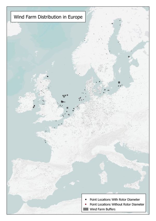
Upps al a U niversity log oty pe

                            Collision Risk for Migratory Birds Facing Wind Energy
                            Installations in Europe in Relation to Wind Energy Production
                            Damire Ariel Haydee Rojas Tito

Abstract
The increasing presence of wind energy installations is faced with citizen and political resistance
often founded on the potential damage these can impose on fauna such as birds. This resistance
is an obstacle to the necessary introduction of more weather-based renewable electricity sources
due to the consequences of fossil-fuel electricity generation. However, if the introduction of more
wind energy installations is to continue, this must also not be at the expense of wildlife. This
project seeked to verify the existence of bird-turbine collision risk and to identify high collision risk
zones in the temporal and spatial scale for Afro-Palaearctic migratory birds flying through Europe.

      Collision risk was assumed as the presence of birds through the swept area of turbines.
The migratory movement of birds was obtained from an interpolation of a geostatistical model and
data from 37 weather radars for the dates 13 February 2018 to 1 January 2019. The data is given
as a volumetric flow across a 0.25° grid. The volumetric distribution of wind energy installations
was derived from a database of 23145 installations and a self-sourced turbine database of 589
turbine models. This distribution is presented as both a high-resolution map covering the
European continent and as a swept area density map. The volumetric bird flow was multiplied by
the swept area density to obtain values for birds at risk of collision in a 0.25° grid cell. Birds were
not considered at risk when the average wind speed in the cell was outside the cut-in and cut-out
wind speed region for the turbines (i.e. not between 3 m/s and 24 m/s).

      The potential electricity production per 0.25° grid cell was also estimated. This was achieved
by assigning power curves from a database to the wind energy installations and assigning a mean
power curve to the entries missing a specific turbine model. The wind velocities were hourly
average values for the dates 13 February 2018 to 1 January 2019 from the ERA5 reanalysis. A
calculation of energy per bird at risk in [TJ/bird] was also done.

      Four high collision risk spatial zones were explored in detail by use of a map compiled in
QGIS and their proximity to or overlay with protected bird habitat sites discussed. Temporally,
date ranges when bird collision is highest were obtained for the four country sub-region in 2018.
The possibility of curtailment is briefly discussed.

                                           Fac ulty of Sci enc e and Technol ogy, U ppsal a U niv ersity. Err or! R efer en ce sou rce not fou nd.. Supervis or: Dr. Silke Bauer, Subject reader: Prof. Jan Sundberg, Exami ner: Dr. Irina Temiz

                             Faculty of Science and Technology
                                  Uppsala University, Uppsala

                       Supervisor: Dr. Silke Bauer Subject reader: Prof. Jan Sundberg
                                         Examiner: Dr. Irina Temiz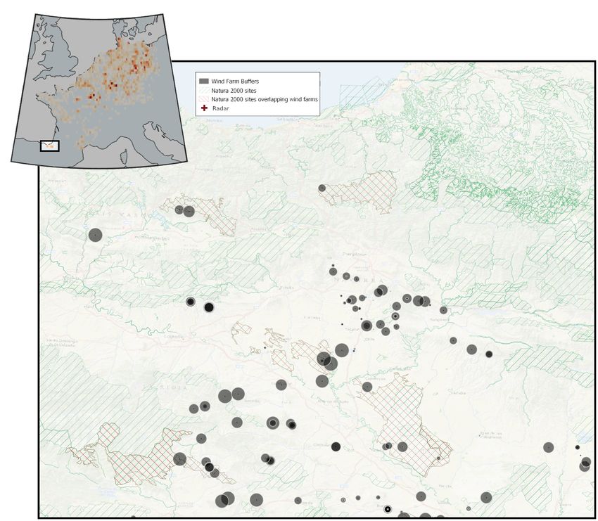
II

Acknowledgements

I have been beyond lucky in having Silke Bauer as my supervisor. I am grateful for her
scientific and academic guidance across all stages of my master thesis. But mostly, I
am grateful for the support and understanding she has shown me through the several
(sometimes strange, sometimes serious) challenges I encountered in the past year. I had
the opportunity to work alongside Raphaël Nussbaumer for only a couple of months,
which was more than enough to know him as a talented and dedicated scientist whose
presence dynamized this project. I very much look forward to reading about his future
research.

   I would like to thank Jan Sundberg as well, foremost for granting me endless coffee
access but also for his thoughtful corrections to this manuscript and for supporting my
interest in birds since our first conversation. Like many others in my Masters programme,
I am thankful to student counsellor Juan de Santiago, who always had a solution for the
many problems we all have presented him. I would also like to thank the professors and
doctoral students within the Division of Electricity that answered some wide-ranging
questions related to this master thesis work.

   I am grateful to both my families, those in Peru but also the friends that take over the
role of family when one is away from home. Gizem, Sherif, Anara and Nastasia are the
sisters I never had. I am also grateful to Alexander, whose advice and company have
made the challenges in the past year easier to handle.

   And last but not least: the mallards, crows, blue tits, blackbirds, starlings and many
others that sometimes allow me into their world, which enriches my own. Except for
robins, which I have decided do not exist.

Uppsala University                                       Damire Ariel Haydee Rojas Tito
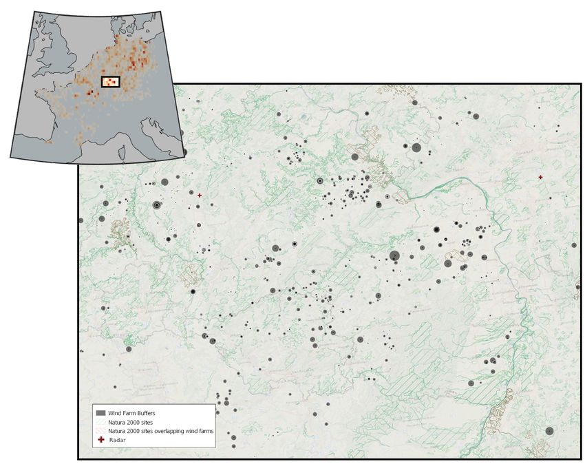
Table of Contents                                                                                III

Table of Contents

Abstract                                                                                         II

Acknowledgements                                                                                 II

List of Tables                                                                                  VI

List of Figures                                                                                 VII

List of Acronyms                                                                                IX

1   Introduction                                                                                  1
    1.1   Objectives . . . . . . . . . . . . . . . . . . . . . . . . . . . . . . . . . . . .      1
    1.2   Scope . . . . . . . . . . . . . . . . . . . . . . . . . . . . . . . . . . . . . . .     2
    1.3   Limitations . . . . . . . . . . . . . . . . . . . . . . . . . . . . . . . . . . . .     2
    1.4   Report Structure . . . . . . . . . . . . . . . . . . . . . . . . . . . . . . . . .      3

2   Background                                                                                    4
    2.1   Bird Migration . . . . . . . . . . . . . . . . . . . . . . . . . . . . . . . . . .      4
          2.1.1   The Afro-Palaearctic bird migration system . . . . . . . . . . . . .            4
          2.1.2   Decline of migratory birds and their conservation . . . . . . . . .             6
    2.2   Radar-based Monitoring . . . . . . . . . . . . . . . . . . . . . . . . . . . .          7
    2.3   Bird Migration Movement Data . . . . . . . . . . . . . . . . . . . . . . . .            7
    2.4   Bird and Turbine Collision . . . . . . . . . . . . . . . . . . . . . . . . . . .        9
    2.5   Wind Energy . . . . . . . . . . . . . . . . . . . . . . . . . . . . . . . . . . .      10
          2.5.1   Wind Turbines . . . . . . . . . . . . . . . . . . . . . . . . . . . . .        10
          2.5.2   Wind Farm Location — Offshore and Onshore . . . . . . . . . . .                12
          2.5.3   Wind Turbine Array in Wind Farms . . . . . . . . . . . . . . . . .             13
    2.6   Curtailment of Wind Turbines . . . . . . . . . . . . . . . . . . . . . . . . .         14
          2.6.1   Curtailment implications at turbine level . . . . . . . . . . . . . .          14

3   Methodology                                                                                  16
    3.1   Stage 1 — Wind Farm Distribution and Characteristics . . . . . . . . . .               17
          3.1.1   The Wind Power Database . . . . . . . . . . . . . . . . . . . . . .            17
          3.1.2   Adding Rotor Diameter Values to The Wind Power database . . .                  18
          3.1.3   Creating surface polygons from point locations . . . . . . . . . .             20
    3.2   Mapping the Wind Facilites . . . . . . . . . . . . . . . . . . . . . . . . . .         21
          3.2.1   Map Projection . . . . . . . . . . . . . . . . . . . . . . . . . . . . .       21

Uppsala University                                            Damire Ariel Haydee Rojas Tito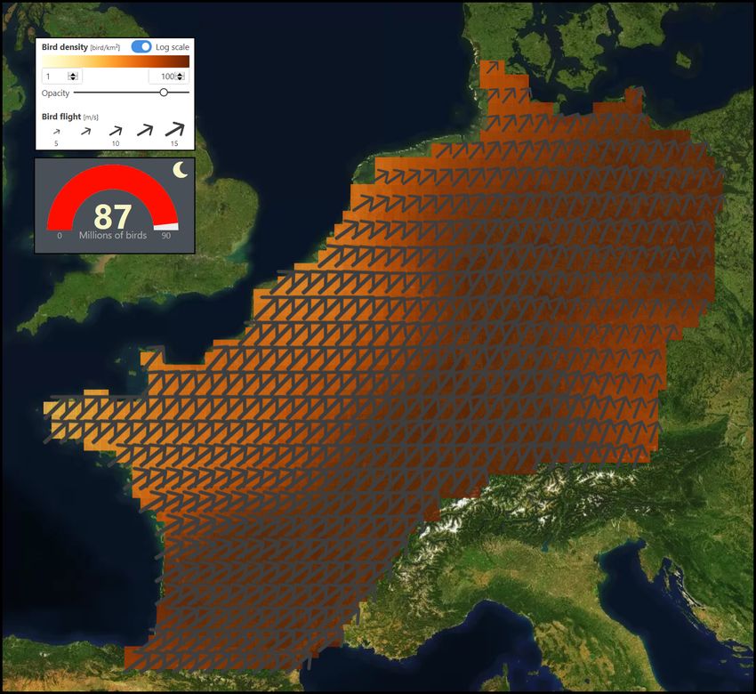
Table of Contents                                                                                IV

          3.2.2   Wind Farm Radius . . . . . . . . . . . . . . . . . . . . . . . . . . .         21
    3.3   Comparing calculated buffer zones with available real wind farm polygons 25
    3.4   Stage 2 — Linking bird migration patterns to wind farm data so as to
          identify spatio-temporal risk zones. . . . . . . . . . . . . . . . . . . . . .         25
          3.4.1   Wind Energy Installation Filtering . . . . . . . . . . . . . . . . . .         25
          3.4.2   Matching Bird Flow and Swept Areas . . . . . . . . . . . . . . . .             25
    3.5   Stage 3 — The estimation of energy production and comparison with
          birds at risk. . . . . . . . . . . . . . . . . . . . . . . . . . . . . . . . . . . .   26
          3.5.1   The ERA5 reanalysis . . . . . . . . . . . . . . . . . . . . . . . . . .        26
          3.5.2   Wind Speeds at Hub Height . . . . . . . . . . . . . . . . . . . . . .          27
          3.5.3   Power Curves . . . . . . . . . . . . . . . . . . . . . . . . . . . . . .       28

4   Results and Analysis                                                                         30
    4.1   Stage 1 — Wind Farm Distribution and Characteristics . . . . . . . . . .               30
          4.1.1   Natura 2000 Protected Sites and Wind Farm Areas . . . . . . . . .              30
          4.1.2   Wind Turbine Database . . . . . . . . . . . . . . . . . . . . . . . .          32
          4.1.3   Comparing calculated wind farm radii with real wind farm polygons 35
          4.1.4   Swept Area Density . . . . . . . . . . . . . . . . . . . . . . . . . .         36
    4.2   Stage 2 - Identifying spatio-temporal risk zones for migratory birds . . .             37
          4.2.1   Bird Density Variation . . . . . . . . . . . . . . . . . . . . . . . . .       37
          4.2.2   Spatial Variation of Bird Collision Risk . . . . . . . . . . . . . . .         37
          4.2.3   Temporal Variation of Bird Collision Risk . . . . . . . . . . . . . .          42
    4.3   Stage 3 — The estimation of energy production and comparison with
          birds at risk . . . . . . . . . . . . . . . . . . . . . . . . . . . . . . . . . . .    44

5   Discussion                                                                                   47
    5.1   Risk of Collision Calculation . . . . . . . . . . . . . . . . . . . . . . . . . .      47
    5.2   Wind Turbines as a Standing Structure . . . . . . . . . . . . . . . . . . . .          47
    5.3   Installation of Turbines in Protected Areas . . . . . . . . . . . . . . . . . .        47
    5.4   Risk Zones with Wind Energy Installations Outside of Protected Areas .                 48
    5.5   Temporal Risk Zones . . . . . . . . . . . . . . . . . . . . . . . . . . . . . .        49
    5.6   Distribution of Bird Density, Swept Area Density and Bird Collision Risk               49
    5.7   Birds Associated to the Topography of Risk Zones . . . . . . . . . . . . .             49
    5.8   Birds at Risk and Energy Trade-off . . . . . . . . . . . . . . . . . . . . . .         49
    5.9   Turbine curtailment challenges . . . . . . . . . . . . . . . . . . . . . . . .         50
    5.10 The impact of wind energy on birds as a negative externality . . . . . . .              50
    5.11 Sources of Error . . . . . . . . . . . . . . . . . . . . . . . . . . . . . . . . .      51

6   Conclusion and Further Work                                                                  52
    6.1   Conclusions . . . . . . . . . . . . . . . . . . . . . . . . . . . . . . . . . . .      52
          6.1.1   Development of a method for collision risk zone assessment . . .               52
          6.1.2   Spatio-temporal occurence of collision risk . . . . . . . . . . . . .          52

Uppsala University                                             Damire Ariel Haydee Rojas Tito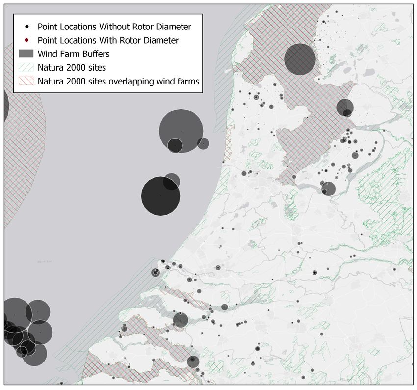
Table of Contents                                                                               V

         6.1.3   Electric energy and birds at risk . . . . . . . . . . . . . . . . . . .        52
         6.1.4   Curtailment to mitigate collision risk . . . . . . . . . . . . . . . .         52
   6.2   Recommendations for Further Work . . . . . . . . . . . . . . . . . . . . .             52
         6.2.1   Corroboration with Field Data . . . . . . . . . . . . . . . . . . . .          53
         6.2.2   Multi-Criteria Decision Analysis . . . . . . . . . . . . . . . . . . .         53
         6.2.3   Extended area . . . . . . . . . . . . . . . . . . . . . . . . . . . . . .      53
         6.2.4   Offshore wind farms . . . . . . . . . . . . . . . . . . . . . . . . . .        53
         6.2.5   Peak migration date variation between years . . . . . . . . . . . .            53
         6.2.6   Turbine properties within the risk zones . . . . . . . . . . . . . . .         53
         6.2.7   Simulation of turbine shut-down at different time scales for a risk
                 area . . . . . . . . . . . . . . . . . . . . . . . . . . . . . . . . . . . .   53

Bibliography                                                                                    54

Appendices                                                                                      59

A Wind Farm Data Sources                                                                        59

B Collision Probability Calculation                                                             61

Uppsala University                                            Damire Ariel Haydee Rojas Tito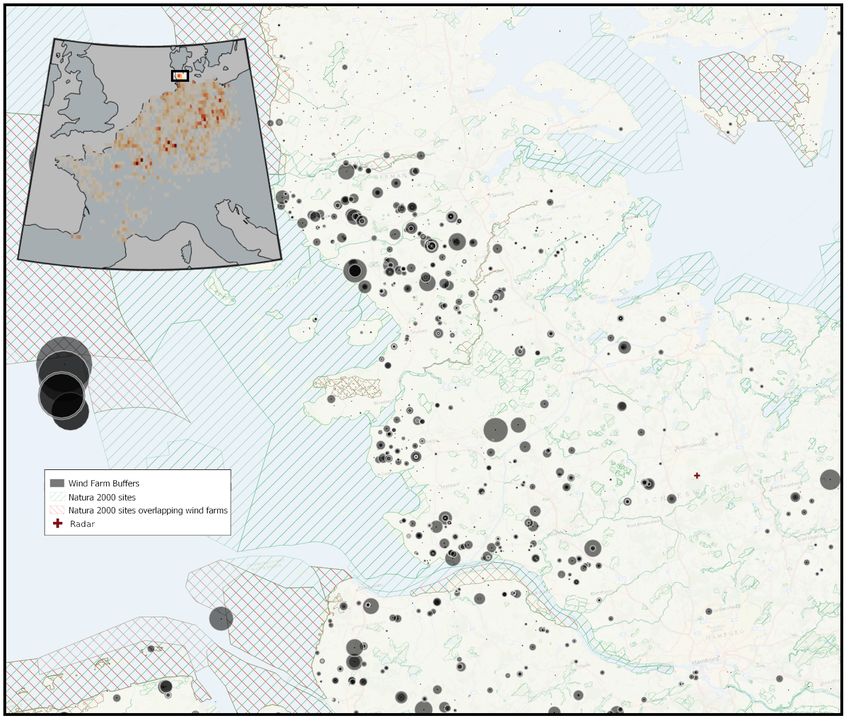
List of Tables                                                                        VI

List of Tables

Table 2.1: Table of parameters that influence collision risk by various guidances .   10

Table 3.1: Table of relevant attributes from The Wind Power Database . . . . . .      18

Uppsala University                                     Damire Ariel Haydee Rojas Tito
List of Figures VII
List of Figures
Figure 2.1: The Afro-Palaearctic Migration System . . . . . . . . . . . . . . . . . 5
Figure 2.2: Natura 2000 Conservation Area Network Map . . . . . . . . . . . . . 6
Figure 2.3: Map of 37 weather radars used to obtain bird migration data . . . . 8
Figure 2.4: Bird migratory density map by Nussbaumer et al (2020) for peak 2018
spring migration . . . . . . . . . . . . . . . . . . . . . . . . . . . . . . 8
Figure 2.5: Bird Density Vertical Profile Time Series for Belgian Radar During
Peak Autumn Migration in 2018 . . . . . . . . . . . . . . . . . . . . . 9
Figure 2.6: Horizontal Axis Wind Turbine . . . . . . . . . . . . . . . . . . . . . . 11
Figure 2.7: Power Curve Plot for Nordex N90 . . . . . . . . . . . . . . . . . . . . 12
Figure 2.8: Wind Farm Grid Array . . . . . . . . . . . . . . . . . . . . . . . . . . 13
Figure 3.1: The parameters needed for the establishing of a collision window of
a wind turbine . . . . . . . . . . . . . . . . . . . . . . . . . . . . . . . 17
Figure 3.2: The surface area covered by a single stand-alone turbine . . . . . . . 20
Figure 3.3: Two-turbine (n T =2) Wind Farm . . . . . . . . . . . . . . . . . . . . . . 22
Figure 3.4: Four-turbine (n T =2) Wind Farm . . . . . . . . . . . . . . . . . . . . . 23
Figure 3.5: Nine-turbine (n T =9) Wind Farm Array . . . . . . . . . . . . . . . . . 24
Figure 3.6: Wind shear vertical profile . . . . . . . . . . . . . . . . . . . . . . . . 27
Figure 3.7: Normalized Power Curves . . . . . . . . . . . . . . . . . . . . . . . . 28
Figure 3.8: Median Power Curve . . . . . . . . . . . . . . . . . . . . . . . . . . . 29
Figure 4.1: Compiled Wind Farm Distribution Map . . . . . . . . . . . . . . . . . 31
Figure 4.2: Detail on Netherlands map with wind farms, Natura 2000 sites and
their overlapping areas . . . . . . . . . . . . . . . . . . . . . . . . . . 32
Figure 4.3: Turbine Models per Turbine Capacity . . . . . . . . . . . . . . . . . . 33
Figure 4.4: Number of Wind Farms per Turbine Capacity in Europe . . . . . . . 34
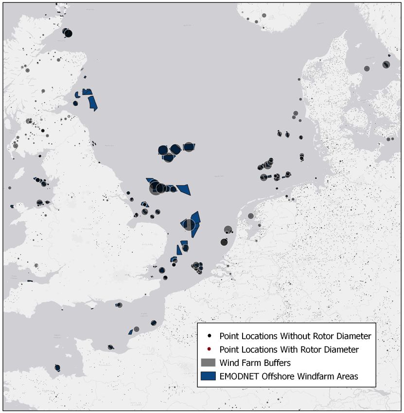
Figure 4.5: North Sea Detail of Wind Farm Map Including Offshore Wind Farm
Polygons from EMODNET . . . . . . . . . . . . . . . . . . . . . . . . 35
Figure 4.6: Wind Turbine Swept Area Density Heat-Map . . . . . . . . . . . . . 36
Figure 4.7: Heat-map illustrating the bird density per cell during 2018 . . . . . . 37
Figure 4.8: Heat-map illustrating the potential total number of birds per cell at
risk of turbine collision during 2018 . . . . . . . . . . . . . . . . . . . 38
Figure 4.9: First bird collision risk zone detail in Grand Est, France . . . . . . . . 39
Figure 4.10: Second bird collision risk zone detail in Saarland and Rheinland-Pfalz,
Germany . . . . . . . . . . . . . . . . . . . . . . . . . . . . . . . . . . 39
Uppsala University Damire Ariel Haydee Rojas Tito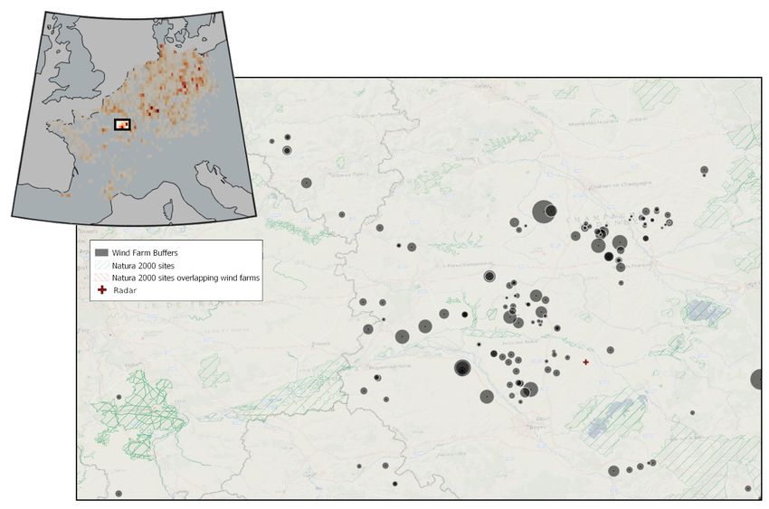
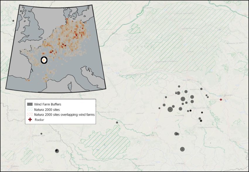
List of Figures                                                                          VIII

Figure 4.11: Third bird collision risk zone detail in Centre-val de Loire, France .       40
Figure 4.12: Fourth bird collision risk zone detail in Centre-val de Loire, France .      41
Figure 4.13: Fifth bird collision risk zone detail in Navarra, Spain . . . . . . . . .    41
Figure 4.14: Sixth bird collision risk zone detail in Schelswig-Holstein, Germany         42
Figure 4.16: Heat-map showing electric energy per bird at risk for 2018 . . . . . .       44
Figure 4.15: Hourly Birds at Risk of Collision Across 2018 . . . . . . . . . . . . .      45
Figure 4.17: Potential Electricity Production and Birds at Risk of Collision . . . .      46

Uppsala University                                       Damire Ariel Haydee Rojas Tito
Nomenclature                                                                       IX

Nomenclature

η         Efficiency of Wind Turbine

ρ         Density of Air

ρbird     Bird Density per Grid Cell

Arotor Swept Area of Turbine Rotor

Cp        Power Coefficient of the Turbine

Dr        Turbine Rotor Diameter

Hh        Turbine Hub Height

l f arm   The Length of the Square Area a Wind Farm Occupies

nT        Number of Turbines in a Wind Energy Installation

Pmax      Maximum Power Output of a Turbine

Pout      Output Power of a Wind Turbine

Qbird     Bird flow at Turbine Height

r f arm   Wind Farm Radius
     T =x
r nf arm  Radius of a Wind Farm with ’x’ Number of Turbines

rwt       Ratio of Bird Density at Wind Turbine Hub Height

Scross Crosswind Spacing for Wind Turbines in a Wind Farm

Sdown Downwind Spacing for Wind Turbines in a Wind Farm

UHh       Wind speed at Hub Height

Uin       Cut-in Wind Speed of a Turbine

Uout      Cut-out Wind Speed of a Turbine

Uwind Wind Speed Incident on Turbine Rotor

vbird     Bird Flight Speed Vector

z         Height Above Surface for Wind Profile Power Law Calculation

zr        Height ’r’ above surface for Wind Profile Power Law Calculation

Uppsala University                                      Damire Ariel Haydee Rojas Tito
Introduction 1 1 Introduction Wind energy is a large contributor to the share of renewable electricity production. In order to reach the European Union’s target of a minimum 32% share of renewable energy consumption by 2030 [1], wind farms are set to become more present across land and marine territory. This is a desirable target, as the consequences of fossil fuel dependency for electricity production become more apparent. However, many citizens and some pro-fossil-fuel politicians are opposed to the increasing number of wind farms [2] [3]. A central motivation in their opposition is the environmental impact wind turbines can have on wildlife, particularly birds [3]. This impact can arise from the conflict between birds and wind farms installed in stationary habitats relevant to the life-cycle of birds but also from collision between air-borne birds and rotating turbine rotors [4]. In the case of the first conflict described, schemes such as Natura 2000 grant protec- tion to resident, breeding and wintering bird habitats in Europe. While this protection of habitats is important, birds are not always sedentary or bound to one habitat. More often than not, birds migrate between habitats as the seasons and their needs change. Migratory birds make up around 40% of the world’s bird species [5] and such birds could be at risk in airspace that they occupy temporarily. This could particularly be the case during concentrated bird migration, which occurs when a large proportion of migratory birds set flight in the spring or autumn migrations. These temporary air-spaces could be a significant contributor to the collision risk conflict, as this is when many birds are airborne. These spaces are, however, harder to identify as it requires knowledge of the volumetric distribution of bird movement as well as their timing along with the volumetric distribution of the rotors of wind turbines. Recent usage of radar can aid in identifying this distribution of birds in the air across the year, as detailed in [6] and [7]. In combination with knowledge of the volumetric distribution of wind turbine rotors, an assessment can be made on when and where an elevated risk of bird-turbine collision exists. Moreover, a trade-off might be identified between saving important wildlife while still sustaining energy production. 1.1 Objectives A main objective of this project is to explore the risk of collision between birds and wind energy installations in the European continent; to assess where and when this risk exists Uppsala University Damire Ariel Haydee Rojas Tito
Introduction                                                                               2

if it exists at all.

   As a concrete output, a risk map of central Europe for migratory bird collisions will
be compiled for the year 2018. This map can be of relevance to conservationists and
wind energy planners to assess and mitigate collision between migratory birds and
existing or planned wind energy installations.

   A secondary objective is to explore this risk in relation to electricity production from
the turbines in question. The project will estimate the total electricity production within
a central European sub-region and then compare this with the number of birds at risk.
This comparison will be made so as to analyse the trade-off from wind farm curtailment
at times of high collision risk. The applicability of curtailment within the regulatory and
technical constraints will also be briefly discussed.

   This Master thesis project is embedded in GloBAM 1 , a research project involving
collaborators from Switzerland, Belgium, Finland, the Netherlands, the UK and the USA
that make use of radar data for animal movement studies. An important aim within
GloBAM is to evaluate the risk of wind energy installations to migratory birds.

1.2 Scope
The project focused on central European countries and the movement of migratory birds
in the Afro-Palaearctic migration system during the year 2018. While information for
both off-shore and on-shore wind energy installations is sourced and mapped.

   Collision risk will be calculated and mapped across a 0.25° grid cell, which will not
identify individual wind energy installations within each cell. Instead, a more detailed
spatial analysis of risk cells will be done. The temporal analysis will not identify specific
dates as these can vary between years.

1.3 Limitations
Only in-shore wind farms are taken into consideration for collision, due to the bird
migration data being available only for inland flow of birds.

   Birds are modeled as a volumetric flow rather than as individual birds. The project
has aimed to calculate the number of birds at risk of collision, rather than the number
of birds that are guaranteed to collide. Moreover, collision risk is not considered for a
particular species of bird.

 1 https://globam.science

Uppsala University                                        Damire Ariel Haydee Rojas Tito
Introduction                                                                              3

   The project has only considered collision with the sweeping rotor of the turbine, not
with the tower or other tall structures that might be part of a wind farm installation.

1.4 Report Structure
The report begins by introducing aspects of the different knowledge spheres of bird
migration and wind energy that are relevant to understand their conflict. The method-
ology is then split into three stages. The results and analysis are also presented for the
three stages. Particular matters related to the findings are then discussed, followed
by a conclusion that includes suggestions for further work. The report ends with a
bibliography and two appendices.

Uppsala University                                      Damire Ariel Haydee Rojas Tito
Background                                                                               4

2 Background

In this chapter, an overview of aspects of bird migration and conservation relevant to
this study will be presented. Some background on wind energy generation and the
wind resource will also be presented. The chapter will include some information on the
challenges from curtailment of wind energy production.

2.1 Bird Migration
The changing of seasons brings about variation in available resources, which mismatch
the varying needs of birds across the year. What constitutes a good breeding and nesting
ground during a period of the year can become unsuitable at other times. In response to
the varying availability of resources, many bird species adopt a migratory life-style [8]
and migrate twice a year between e.g. non-breeding and breeding areas. The number of
individuals involved in these migrations is impressive; it is estimated to total around 50
billion individuals globally [9] and between Europe and Africa, an approximate 2 billion
song-birds [10].

   The migration of birds connects ecosystems and food webs. Birds move seeds, nutri-
ents and also parasites from otherwise unconnected regions. Migratory birds are thus
key habitants of ecosystems and have an influence on the anthroposphere [11]. Although
most bird species are active during the day, during migration they change to nightly
flights [12].

   Song-birds fly by flapping, which is energy-demanding. Thus, they take shorter
routes and migrate on a broad front, with some flight concentration found on mountain
passes or coasts not too far off their main direction [9].

2.1.1 The Afro-Palaearctic bird migration system

Many bird species naturally occurring in European territory (land and sea) are migratory
[13]. Their migration distances vary but cover journeys across latitudes of breeding
grounds in Europe and non-breeding grounds in the sub-Sahara [10]. Birds making
these journeys compose the Afro-Palaearctic bird migration system which, with over two
billion individuals covering over 100 species, is the largest landbird migration network
in the world [14]. Of these individuals, over 80% are songbirds and near-passerine bird

Uppsala University                                           Damire Ariel Haydee Rojas Tito
Background                                                                            5

species [14].

   This journey between Europe and Africa requires long-distance migrant species to
cross the Mediterranean Sea. As this can be an energetically costly journey, individuals
will tend to avoid extended sea-crossings and therefore funnel into particular routes
where the continents are closer together. Consequently, the Afro-Palaearctic bird mi-
gration system splits into an Eastern and Western Flyway. This project focuses on the
Western Flyway, which in Europe goes from Scandinavia through to Germany and
southwards towards the Strait of Gibraltar.

Figure 2.1: Map showing some details of the Eastern and Western flyways of the
            Afro-Palaearctic migration system. The funneling between Europe and
            Africa occurs in two directions represented by two arrows, an Eastern flyway
            in blue and the Western flyway in red. It should be noted that the direction
            of the arrows represent movement in the Autumn. This direction is opposite
            in the Spring.[14]

Uppsala University                                     Damire Ariel Haydee Rojas Tito
Background 6
2.1.2 Decline of migratory birds and their conservation
Bird populations have been on a decline [13] and as a response to this, the European
Union issued the Birds Directive. It aims to protect "all of the 500 wild bird species
naturally occurring in the European Union" [13].
Acknowledging habitat loss as a major threat to wild birds, an important achievement
of the Birds Directive has been the creation of a network of Special Protected Areas
which have all since been included in the Natura 2000 ecological network [13]. This
extensive network that covers 18% of the EU’s land area and around 6% of its marine
territory can be seen in Figure 2.2.
The Birds Directive also lists 194 bird species and sub-species of particular concern.
Of these, 54 species have been assigned and benefit from Species Action Plans 1 .
Figure 2.2: A map showing the European Natura 2000 Network of Special Protection
Areas, a product of both the Birds Directive (areas in in red) and the Habitats
Directive (areas in blue). The areas have different importance to the lifetime
of birds that live inland and/or at sea. [15]
1a
list of the species can be found at
https://ec.europa.eu/environment/nature/conservation/wildbirds/action_plans/index_en.
htm
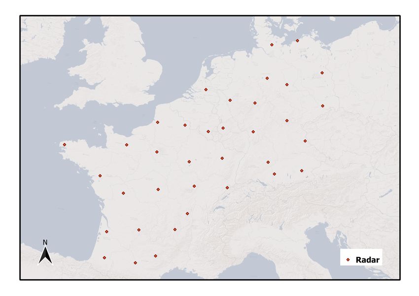
Uppsala University Damire Ariel Haydee Rojas TitoBackground 7 These sites grant spatial protection to birds during times when they are not in movement such as breeding, wintering and permanent living territories. 2.2 Radar-based Monitoring The volumetric flow of birds used in this project was estimated from radar measurements. Radar technology gives the same benefits to bird monitoring that it has allowed other activities, making observation possible at all hours and a wide variety of weather conditions. Also, it can locate an object to altitudes and distances not possible to the human eye. It has thus been valuable in providing information on the biomass/numbers of birds, their speed, direction and altitude of bird flight at conditions not previously possible. However, it should be noted that radar is less able than the human eye in distinguishing between bird species. 2.3 Bird Migration Movement Data The bird migration movement data used in this project were obtained by the method- ology described in [6] and [7] for the period of 13 February 2018 to 1 January 2019 (non-inclusive). The original data originate from 37 weather radars across central Eu- rope (see Figure 2.3) and were made available to the European Network for the Radar surveillance of Animal Movement (ENRAM) 2 . First, the model combines the spatio-temporal structure of bird migration from punc- tual radar measurements (given by the radars as an average for bird density and flight speed) with a Gaussian process regression to estimate bird densities [birds/km2 ] at any location in space and time (i.e. a spatio-temporal grid) [6]. Interpolation was done within a 0.25° grid 3 covering the territory between latitudes 43°to 55° and longitudes -5° to 16° (this area covers the radars in Figure 2.3), additionally it was only done for grid "nodes" that fit the criteria of being over land and within 150 [km] of a radar. Moreover, time periods with rain intensity over 1mm/hr and during daytime were excluded. Through this process a resolution of 0.25° per 15 min was achieved [6] for bird density and flight velocity at the horizontal level. The resulting maps are available at https://birdmigrationmap.vogelwarte.ch/2018/. A still picture for the spring peak migration of 2018 (29 Mar 2018) is shown in Figure 2.4. 2 https://www.enram.eu/ 3 At 50°N latitude, 0.25° is equivalent to 27.8 [km] Uppsala University Damire Ariel Haydee Rojas Tito
Background                                                                               8

Figure 2.3: The 37 weather radars used in [7] are depicted by red dots in the map. The
            radars are located in Belgium, The Netherlands, Germany and France which
            are areas that correspond to the Western Flyway. This map was compiled
            from information available in [16].

Figure 2.4: A still picture of the bird density and flight velocities interactive map found
            at [17] for the peak spring migration in 2018 (29 Mar 2018). The dimension of
            the dark grey arrows scales up with increasing bird velocity and points in
            the direction of flight. The bird density is shown as a gradient between light
            yellow (low density) and dark red (high density).

Uppsala University                                       Damire Ariel Haydee Rojas Tito
Background 9
The vertical distribution of birds was achieved in [7] by considering nocturnal broad-
front bird migration as a fluid. The results are analysed and shown in [7] as birds taking
off, landing and entering. Bird densities as a vertical profile time series can be seen per
radar on [18]. A sample of these vertical profiles is shown in Figure 2.5.
Figure 2.5: A vertical profile of bird density over ground is shown in a gradient going
from dark purple (low density) to yellow (high density). This vertical profile
corresponds to the dates around peak autumn migration in 2018 and is only
for one radar in Belgium. This take-out of the vertical profiles available for
2018 and for many radars was taken from [18].
2.4 Bird and Turbine Collision
It is difficult to obtain an exact number of the birds colliding with wind turbines. This
figure is often obtained via carcass searches, which have inherent shortcomings as they
are not standardised and carcasses can be eaten before found or not be spotted by those
looking for it [19] [20].
A collision probability value can also be complicated to compute as it has many
influential factors. There are several guidelines to calculate collision probability, which
take into consideration many of the parameters that influence potential collision. An
example of a collision probability calculation by the Scottish Natural Heritage body
[21] is shown in Appendix B. As a summary, Table 2.1 is a compilation of the many
parameters required from the guidances in [4], [21] and [22].
The guidelines propose various calculation procedures to obtain a figure for colli-
sion risk probability. However, taking into account the many parameters that go into
calculating this figure, these calculations could prove inaccurate.
Uppsala University Damire Ariel Haydee Rojas TitoBackground 10
Table 2.1: Table categorising the parameters that influence bird-turbine collision risk by
[4], [21] and [22]. Accurate values of these parameters are needed in the
calculations they suggest.
Wind Farm Environment Bird Bird Flight
Number of rotors Visibility Length of bird Time spent flying
Maneuverability Altitude and range
Swept area of rotors Time of day
of bird of flight altitude
Number of Avoidance
Topography
blades in rotor behaviours
Depth of rotor Weather Conditions
2.5 Wind Energy
This sub-section will cover aspects of wind turbines and wind farms that are relevant
to exploring their physical conflict with bird migration. Beyond the physical conflict,
electricity production and curtailment challenges will be described to fulfill the aim of
exploring the relation between birds at risk and potential wind energy production.
2.5.1 Wind Turbines
Most wind farms in Europe make use of horizontal axis wind turbines [23]. A diagram
of such a turbine, along with its components, can be seen in Figure 2.6.
The amount of power generated by a wind turbine depends on the rotor and its
interaction with incident wind [24]. This relationship is expressed mathematically in
Equation 2.1
1 3
Pout = · ρ · Arotor · C p · η · Uwind (2.1)
2
where Pout is the output power in [W], ρ is the air density in [kg/m3 ], Arotor is the
swept area of the rotor in [m2 ], C p is the power coefficient of the turbine [unitless], η is
the efficiency of the turbine [%] and Uwind is the wind speed incident on the rotor in
[m/s].
While the magnitude of Pout is directly proportional to all parameters in the equation,
maximizing Pout is usually done by increasing Arotor and installing wind farms in areas
with a high occurrence of high wind speeds (Uwind ).
Uppsala University Damire Ariel Haydee Rojas TitoBackground 11
Figure 2.6: Diagram of the common components that make a Horizontal Axis Wind
Turbine, showing main mechanical and electrical parts. The mechanical
parts being the foundation, rotor, tower, nacelle, drive train and yaw system
while the electrical parts are the generator and the balance of the electrical
system (e.g. a transformer). The turbine can yaw about the vertical axis (i.e.
the tower) so the rotor faces the predominant wind direction. [25]
Equation 2.1 plots the behaviour of a turbine after a cut-in wind speed Uin and before
a cut-out wind speed Uout . The overall power curve of a wind turbine follows the
expression in Equation 2.2:
0, U < Uin
Pout (U ) = Pout , Uin ≤ U ≤ Uout (2.2)
P , U ≥ U
max out
A sample power curve is shown in Figure 2.7. The curve corresponds to the Nordex
N90 turbine, plotted by power curves available in the pcurves library in R.
Uppsala University Damire Ariel Haydee Rojas TitoBackground 12
Figure 2.7: Power Curve plot for Nordex N90, showing the power output as a function
of the incident wind speed. The turbine rotor is static below the minimum
cut-in wind speed value and so the power output is zero. At the cut-in wind
speed, the rotor starts rotating and electricity is produced by the generator.
The power output keeps increasing aa a ratio of the cube of the incident
wind speed. When wind speeds become too high, the wind turbine shuts
down (e.g. by yawing) at a cut-out wind speed so as to prevent damage.
Trends of wind turbines
To increase the rotor swept area (Arotor ), the wind turbine manufacturing industry shows
a long-term trend to increase rotor diameter, with 87% of turbines installed in the US in
2018 having at least 110 [m] in rotor diameter [26] and wind turbines in Europe showing
a trend for bigger rotors as well [27].
As for adapting turbines to increase the incident Uwind , hub height of wind turbines
are increasing [26]. This is done because wind speeds tend to increase with altitude,
where there is less influence from friction with ground surface.
2.5.2 Wind Farm Location — Offshore and Onshore
The installation of wind farms in either onshore or offshore areas has benefits and disad-
vantages. Offshore windfarms benefit from higher wind speeds and less NIMBY (the
’Not in My Backyard’ concept) objections from residents [28]. However, offshore wind
farms require significant logistics for installation and maintenance and often require the
installation of seabed cables for grid connectivity [24]. Onshore windfarms are closer
to grid connections (although not always to transmission standards) and are usually
more accessible for installation and maintenance [23]. They, however, tend to have lower
average wind speeds and also suffer more from NIMBY opposition [28].
Uppsala University Damire Ariel Haydee Rojas TitoBackground 13
In Europe, while offshore projects are gaining approval and have an increasing
presence (particularly in the UK, Germany, Denmark and Belgium), 76% of new wind
installations in 2019 were onshore. Onshore wind farm installations are still dominant
both in terms of capacity and production [27]. This is also the case in the United States,
where only one offshore wind project is operational [26].
2.5.3 Wind Turbine Array in Wind Farms
Wind turbines have placement requirements when installed as a group. A main reason
for this is wake effects. Once a turbine takes in energy from the incident wind, there will
be wake effects such as lower wind speeds and turbulence downwind of the turbine. If
another turbine is placed in the path of this wake, losses will be introduced. Wake losses
account for a 5% to 15% reduction in annual energy production and the effect is stronger
at slower wind speeds [24]. Fatigue from turbulence can also damage the turbine in the
long term [24]. Thus, wind farms introduce certain required distances between their
turbines.
A grid-like array pattern for wind turbines can be seen in Figure 2.8. This pattern is
common in offshore wind farms; however, at land, grid-like turbine array patterns are
not always common due to topography. Regardless of pattern, downwind spacing and
crosswind spacing must be kept at a minimum so as to reduce wake effects.
Figure 2.8: Grid array of wind turbines within a wind farm„ with the turbine shown as
white circles and the wind farm as a dotted circle outline. This spacing is
done in order to avoid losses from turbine wake and is most often seen
offshore. [24]
Crossing and downwind spacing are measured in rotor diameters (Dr ). An industry
standard for these is usually 8 · Dr to 10 · Dr in downwind and 5 · Dr in crosswind
Uppsala University Damire Ariel Haydee Rojas TitoBackground 14 direction [24]. Whether a direction is crosswind or downwind is dependent on the direction of the prevailing wind, as seen in Figure 2.8. 2.6 Curtailment of Wind Turbines Curtailment will be briefly explored as a potential solution to reduce the collision risk in this project. Here, some aspects of curtailment will be presented. Curtailment can be described as the scheduled braking of wind turbines [24]. As this stops the rotor from behaving as a spinning disk (i.e. reducing the impact area) and also reduces the force with which a blade can strike a bird, the risks associated with collision could be reduced. However, the shutting down and starting up of a wind turbine has implications not just to the turbine itself but also to the grid it is connected to. Curtailment implications at electrical grid level The electrical supply in a system (consisting of power producers, consumers and the transmission/distribution network) must adhere to quality standards. Voltage should be sinusoidal and, in the European Union, its amplitude must fall at 230 V +10%/6% with a constant frequency of 50Hz [29]. The supply can deviate from these standards when there is a mismatch between demand and generation. The deviation can be affected by the size of the system (larger systems are less affected) and whether the network is of transmission (less deviation) or distribution quality (more deviation). Deviation in quality is also affected by how much reactive and active power reserve a system has [23]. The disconnection of a power plant (i.e. a wind farm) would decrease the generation supply of the system. The time scale of this disconnection and the reserve of the system would determine how well the system could handle this disconnection [23]. As an economical implication, curtailment can increase the levelized cost of energy (LCOE) of wind energy, making it detrimental to its energy market penetration [30]. Wind farms have a high merit order as they have low operational costs. A high merit order means they are operational at almost all times. If they are to be constantly backed up by producers of a lower merit order (which are in turn more expensive), the overall cost of electricity would increase [23]. 2.6.1 Curtailment implications at turbine level The amount of notice that an operator is given to "shut down" a turbine also has impli- cations to the turbine as they have different mechanisms for braking. Turbine braking Uppsala University Damire Ariel Haydee Rojas Tito
Background                                                                               15

is mainly done to protect the wind turbine from wind speeds that are high enough to
damage the turbine or that could destabilize the electrical grid [24]. The shutdown of
a wind turbine can be either planned or reactive, the latter of which meaning that it is
done instantaneously as a reaction to an unscheduled phenomenon. Planned shutdown
(i.e. curtailment) can occur when there are noise or flicker restrictions or because of grid
operation arrangements [23].

Turbine Braking Mechanisms

The braking of wind turbines can be aerodynamic or mechanical. Some recent standards
require that a turbine have two independent braking systems, with one usually being
aerodynamic (in the rotor) and the other mechanical (in the drive train) [24].

   Aerodynamic braking can be done by a combination of one or all of the following
methods [31]:

   1. Drag Devices — Ailerons (similar to those in airplanes) at the turbine blades. These
      are not so common in modern turbines.

   2. Pitching Blades — In pitch-controlled wind turbines, the individual rotor blades
      are pitched out of the wind by hydraulics when the incident wind speeds become
      too high (which is usually determined by a power output monitor).

   3. Yawing — The whole rotor is rotated about its vertical axis so it faces away from
      the wind.

   Aerodynamics braking is considered to be the least damaging to a turbine; it is
also considered safe in stopping turbines operation at unsuitable wind speeds. How-
ever, should aerodynamic brakes fail, or braking need to be done for maintenance, the
mechanical brakes at the drive train are used. Mechanical braking can be one of the
following types:

   1. Disc brake — A hydraulically actuated caliper pushes brake pads against a disc
      that is affixed to the turbine shaft.

   2. Clutch brake — Similar to that of a car, clutch brakes in turbines are actuated by
      springs.

   3. Dynamic brake — After disconnecting the turbine from the electrical grid, power
      is fed to a resistor bank which puts a load on the generator that in turn puts torque
      on the rotor which results in deceleration.

   All the braking methods mentioned can be one of either passive or manually acti-
vated.

Uppsala University                                        Damire Ariel Haydee Rojas Tito
Methodology 16
3 Methodology
The project was divided into three stages.
• Stage 1 — The creation of a surface and vertical distribution map of all wind farms
present in the European continent. This will include sourcing parameters that
are relevant for the next stages, such as for collision and for calculating energy
production.
• Stage 2 — Linking bird migration patterns to wind farm data so as to identify
spatio-temporal collision risk zones.
• Stage 3 — The estimation of energy production and comparison with birds at risk.
Uppsala University Damire Ariel Haydee Rojas TitoMethodology 17
3.1 Stage 1 — Wind Farm Distribution and Characteristics
It is important to know where wind farms are located across the European continent
in order to identify the airspace that they populate. The analysis of bird collision is
volumetric, meaning that it covers air space taken by the turbine that has a vertical and
horizontal component. Thus, while location is a relevant parameter, the dimensional
properties of the turbines within each farm will be necessary to obtain the total surface
distribution of the farms and also the airspace they occupy.
Elevation
(Hh ) + (Dr /2)
Latitude
(Hh ) - (Dr /2)
Longitude
Figure 3.1: Illustration of a wind turbine and its relevant collision window given by the
rotating blades. The attributes required to calculate the area of this window
are the Hub Height (Hh ) and the Rotor Diameter (Dr ) while the airspace
occupied by the rotating rotor (i.e. the collision window area) is
geo-positioned by the latitude, longitude and elevation of the turbine.
The surface distribution is given by the latitude and longitude corresponding to a
wind farm. The area of vertical distribution relevant for collision is the swept area of the
turbines — that is to say the disc of airspace that the rotor covers when rotating. The
lower and upper limits of this disc are obtained via the hub height (Hh ) [m] and the rotor
diameter (Dr ) [m], as detailed in Figure 3.1.
3.1.1 The Wind Power Database
Wind farms across Europe were mapped from the Europe wind farm point location
database by "The Wind Power" 1 . The database version used was that updated by June
2020, which has 23145 wind farm entries. The database has many attributes for wind
farm entries, however those relevant to this project are shown in Table 3.1. The collision
window area (see Figure 3.1) will be determined by WGS84 latitude and longitude
coordinates, the altitude and the hub height.
1 https://www.thewindpower.net
Uppsala University Damire Ariel Haydee Rojas TitoMethodology 18
Table 3.1: A selection of attributes for the wind farm entries to wind farm database from
The Wind Power along with the units they are given in and the corresponding
fill rates for each attribute.
Attribute Unit Fill Rate (%)
Location
City N/A 86
WGS84 coordinates (approximate) Decimal degree 41
WGS84 coordinates (accurate) Decimal degree 54
Altitude/Depth [m] 4
Turbine
Manufacturer N/A 86
Model N/A 79
Hub height [m] 63
Number of turbines N/A 98
System
Total power [kW] 92
Commissioning date yyyy or yy/mm 92
Approved/Construction
Status 100
Dismantled/Planned/Production
The rotor diameter value was missing from the database and (as will be explained
later), this was obtained via the manufacturer, model, number of turbines and total
power attributes.
The manufacturer and model are necessary for Stage 3 of the project, where the power
output of the wind turbines was calculated. This so as to assign the correct power curve
to a wind energy installation’s turbine model.
Missing parameters in The Wind Power database
While the windfarm database from The Wind Power is extensive, it was missing the
critical rotor diameter (Dr ) value. As detailed in Figure 3.1, this value is important for
obtaining the vertical collision window. Additionally, it is important for mapping a
radius around the point locations of the The Wind Power database.
3.1.2 Adding Rotor Diameter Values to The Wind Power database
Many steps were taken in order to populate the The Wind Power database with missing
turbine parameters. All database manipulation was done with the R programming
language.
Uppsala University Damire Ariel Haydee Rojas TitoMethodology 19 Compiling a Wind Turbine Parameter Database The U.S. Wind Turbine Database 2 , a public database by the Department of Energy in the United States, has information on the over 59000 wind turbines installed in the USA. The database became interesting as it includes turbine make and model attributes for the wind farms. In particular, it included the rotor diameter value for its turbines and was thus a good starting point to compile a turbine database. All 164 unique turbine models with corresponding parameters were isolated into a separate database. These models were not enough to cover all the models listed in the The Wind Power database and so the remaining turbine models were entered manually with parameters found in manufacturer websites. This resulted in a database with 589 wind turbine models. The turbine parameters were merged into the The Wind Power database. Rotor Diameter Based on Make and Capacity Only 79% of wind farms have a turbine model listed, meaning they could not be matched with a turbine model in the compiled turbine database. However, some of the wind farm entries have a total power rating and a turbine make (i.e. manufacturer). An individual turbine power rating was derived from the total power rating and number of turbines. In the case where a turbine make only had one turbine model at the individual turbine rating of the farm, the parameters of that model were assumed. In the case where a turbine had more than one turbine model at a turbine rating, the model with the largest rotor diameter was assumed. These cases were annotated in a "notes" column in the database. Detailed Parameters for Territory of Interest Even after the previous work to fill rotor diameter values, some wind energy installations in the territory of interest (detailed in Figure 2.3) had no turbine model. As these installations were important to the study, the turbine models were sourced from various news articles (see Appendix A). When this was the case, a link with the information was added to the "notes" column of the database. Rotor Diameter Based on Hub Height Outside of the territory of interest, and after matching with turbine database and as- sumptions from turbine make and capacity, around 2% of wind energy installation entries still had no rotor diameter value. Some of these entries, however, had a hub 2 https://eerscmap.usgs.gov/uswtdb/ Uppsala University Damire Ariel Haydee Rojas Tito
Methodology                                                                             20

                         Point Location

                                                              Dr /2

Figure 3.2: A single turbine, seen from above, is illustrated in blue. The grey circle
            surrounding it is the surface area it covers when rotating about its vertical
            axis (i.e. yawing). The white dot represents the point location given in
            latitude and longitude.

height value (Hh ).

   Using the compiled turbine database mentioned earlier in this section, a linear rela-
tionship between Dr and Hh with coefficient 0.75 was determined. This is in line with
the value of 0.79 found in [32].

   Thus, in the instances where Hh was given, the value for Dr can be calculated using
this ratio as in Equation 3.1.

                                                  1
                                          Dr =        · Hh                            (3.1)
                                                 0.75

3.1.3 Creating surface polygons from point locations

The wind farm database from The Wind Power provides only point locations for the wind
farms. Point locations do not represent the extent of land surface (and consequently, the
extent of air space) that a wind farm or a wind turbine covers. Thus, the point locations
were converted into surface areas by calculating a wind farm radius (rfarm ) according
to the number of turbines in the wind farm and then mapping a circle with this radius
around the point location given.

Single-standing turbines

There are 8474 wind energy installation entries that consist of a single turbine and are
thus not to be considered as farms. However, they are also not point locations as turbines
rotate 360° about their vertical axis (i.e. they yaw) in order to face the wind direction.
This is graphically represented in Figure 3.2. Thus, for wind energy installations with a
single turbine, a circle with rfarm =Dr /2 will be mapped around the point location. The
resulting surface area is depicted in gray in Figure 3.2.

Uppsala University                                           Damire Ariel Haydee Rojas Tito
Methodology 21
Wind Farms
As described in Section 2.5.3, there are guidelines as to how turbines are arranged within
a wind farm. In order to define a radius around the point locations given, it will be
assumed that the wind farms have turbines arranged as a grid. A prevailing wind
direction for each wind farm entry would be needed in order to establish an accurate
orientation of downwind spacing (Sdown ) and crosswind spacing (Scross ). Instead, a
conservative value of 10 · Dr [m] will be taken for both, this is expressed as:
Sdown = Scross = 10 · Dr [m]
Having a conservative (i.e. generous) distance between the turbines allows for the
variation in grid layout there might be due to topography. A grid layout is more common
among offshore wind farms, whereas onshore farms will have more complex terrain
that would not allow for a uniform grid.
3.2 Mapping the Wind Facilites
Mapping was done with the QGIS software and its Python interface.
3.2.1 Map Projection
The map will be used with the bird migration data described in Section 2.1. This data
is derived from EUMETNET, which uses the ETRS89 Lambert Azimutal Equal Area pro-
jection [33]. As it name implies, this projection is one that avoids area distortion across
latitudes. This is known as an equivalent projection.
This projection uses the "European Terrestrial Reference System 1989" datum, while
the The Wind Power database makes use of the WGS84 datum. Thus, the wind farm
point locations were re-projected onto the ETRS89 Lambert Azimutal Equal Area.
3.2.2 Wind Farm Radius
The polygons for wind farms will be circular areas, mapped by adding a buffer zone
with a radius described as rfarm around the point location given by the The Wind Power
database. The method for turbine mapping will vary depending on the number of
turbines in a wind farm. The shorthand for number of turbines will be described as n T .
Single wind turbine installations
Wind farms with a single turbine will be described as wind farms with n T = 1. Following
the reasoning in Section 3.1.3, the buffer for these wind farms will have a radius of:
Dr
rfarm
n =1
T
=
2
(3.2)
Uppsala University Damire Ariel Haydee Rojas TitoMethodology 22
Point Location
10 · Dr
Dr
Dr
Figure 3.3: Array for wind farms with two turbines (n T =2). The turbine array is seen
from above, with the turbines represented in blue. The wind farm is assumed
to occupy the area shown by the grey rectangle. The dotted circle represents
the buffer zone mapped around the point location as the orientation of the
grey rectangle (i.e. the wind farm) would place it within these bounds.
Wind Farms with Two Turbines
Wind farms with two turbines (n T = 2) will assume the layout in Figure 3.3.
Thus, the radius for these farms will be given by:
rfarm
n =2
T
= D +102· D + D
r r r
rfarm
n =2T
= 6 · Dr (3.3)
Wind farms with Multiple Turbines
Wind farms with n T ≥ 3 look like those illustrated in Figure 3.4 and 3.5 which show
wind farms with n T =4 and n T =9 respectively.
A relationship between the length of the grey square (lfarm ) and the turbine rotor
diameters (Dr ) while keeping the distance of 10 · DR between them is given in Equation
3.4
√
lfarm = (11 n T − 10) Dr (3.4)
These lengths, however, do not give the radius of the wind farm buffer zones. To
obtain the radius, it will be required to use Pythagoras’ Law as follows:
(rfarm · 2)2 = 2 2
√ lfarm + lfarm
2
lfarm 2
+lfarm
rfarm = 2
Uppsala University Damire Ariel Haydee Rojas TitoMethodology 23
Dr
10 · Dr
Point Location
Dr
10 · Dr
Dr Dr
Figure 3.4: Array for wind farms with four turbines (n T =4). The turbine array is seen
from above, with the turbines represented in blue. The wind farm is
assumed to occupy the area shown by the grey square. The dotted circle
represents the buffer zone mapped around the point location. The
dimensions of the sides of the square are given in rotor diameters (Dr ).
Uppsala University Damire Ariel Haydee Rojas TitoMethodology 24
Dr
10 · Dr
Dr
Point Location
10 · Dr
Dr
10 · Dr 10 · Dr
Dr Dr Dr
Figure 3.5: Array for wind farms with nine turbines (n T =9). The turbine array is seen
from above, with the turbines represented in blue. The wind farm is
assumed to occupy the area shown by the grey square. The dotted circle
represents the buffer zone mapped around the point location. The
dimensions of the sides of the square are given in rotor diameters (Dr ).
Uppsala University Damire Ariel Haydee Rojas TitoMethodology 25
√ 2
2·lfarm
rfarm = 2
which, when taking Equation 3.4 gives the following expression:
l 1 √
rfarm = √ rfarm = √ · (11 n T − 10) · Dr (3.5)
2 2
The resulting radii were then plotted as buffer zones around the point locations.
3.3 Comparing calculated buffer zones with available real
wind farm polygons
Many assumptions have been made to obtain the circular polygons around the point
locations. A comparison with some "real" wind farm polygons was made to see how
accurate these derived circular polygons could be. A database with polygons for Eu-
ropean offshore wind farms was obtained from EMODnet Human Activities [34]. These
polygons were overlaid with the buffer zones calculated in Section 3.2 in QGIS, and the
difference in surface areas calculated via the symmetrical difference tool in QGIS.
3.4 Stage 2 — Linking bird migration patterns to wind farm
data so as to identify spatio-temporal risk zones.
The bird migration data used is described in Section 2.3. Bird migration is given as bird
density and bird velocity across a 0.25° grid within the boundaries of latitudes 43°to
55°and longitudes -5°to 16°. A 0.25° grid at 50°N latitude gives a grid with a resolution
of 27.8km x 27.8km cells. A turbine swept area density was calculated per each cell in
the 0.25° grid corresponding to migratory bird data (see Section 2.3). All calculations
were made with MATLAB.
3.4.1 Wind Energy Installation Filtering
The wind farm entries were filtered so that no farms under Construction, Planned, Ap-
proved or Dismantled status were included. This was also the case for turbines without
a value for Latitude and Longitude and any offshore wind farms.
The bird migration data covers a smaller territory within Central Europe bound by
55N, 5W, 43S and 16E. All wind farms outside this area were filtered out.
3.4.2 Matching Bird Flow and Swept Areas
The bird density per grid cell (ρbird ) in [birds/km2 ] was computed and then multiplied
by a flight speed vector (vbird ) in [7]. From this, a bird flow at turbine height (Qbird ) in
Uppsala University Damire Ariel Haydee Rojas TitoMethodology 26
[bird/m2 /hour] was obtained via Equation 3.6, where rwt is the ratio of bird density at
turbine hub height and h is the hub height assumed in the previous ratio.
1
Qbird = ρbird · rwt · · vbird (3.6)
h
Temporally, the bird migration data has a 15 minute resolution. An hourly average
of the previous hour was instead used for the calculations in order to make the results
compatible with the wind velocity data used in Stage 3. has hourly resolution as an
average of the last hour.
As was mentioned in Section 2.4, bird collision probability can be calculated taking
into account many parameters of the turbine, weather, bird and bird flight. However, as
these can lead to a false accuracy, a bird at risk in this project is considered to be a bird
that is within the swept area of the turbine. The birds at risk of collision are calculated
by multiplying the bird flow per grid cell and the turbine swept area density per grid cell.
Additionally, turbines were not considered as a collision risk while they are not
rotating. It was assumed that turbines were only rotating between wind speeds of 3
[m/s] and 24 [m/s]. This wind data was taken from the ERA5 reanalysis, which is
further described in Stage 3.
3.5 Stage 3 — The estimation of energy production and
comparison with birds at risk.
In order to calculate power production for the wind farms during the relevant time
period, it is necessary to have the incident wind speeds at hub height (UHh ) and power
curves for the turbines. The calculations were not done for wind farms under Construc-
tion, Planned, Approved or Dismantled status or turbines without a value for Latitude
and Longitude. Calculations were done with MATLAB.
3.5.1 The ERA5 reanalysis
To get a more accurate measurement of potential electric energy production loss, wind
velocity data for the specific time period (13 February 2018 to 1 January 2019) and region
(bound by 55N, 5W, 43S and 16E) was necessary. This was possible by taking data from
the ERA5 reanalysis [35]. A reanalysis can be interpreted as a weather hindcast, whereby
real wind velocity observations are combined with a physics model to produce a more
expansive dataset for past wind speed values [36].
The ERA5 reanalysis provides wind velocity values on a 0.25 deg (≈ 30km) lat-lon
grid (which matches the bird migration data) at an hourly resolution and at 10 and 100
[m] heights above surface [37]. A study by Olauson et al [38] used ERA5 reanalysis wind
Uppsala University Damire Ariel Haydee Rojas TitoYou can also read