Improving wind farm flow models by learning from operational data
←
→
Page content transcription
If your browser does not render page correctly, please read the page content below
Wind Energ. Sci., 5, 647–673, 2020
https://doi.org/10.5194/wes-5-647-2020
© Author(s) 2020. This work is distributed under
the Creative Commons Attribution 4.0 License.

                    Improving wind farm flow models by learning
                               from operational data
                    Johannes Schreiber, Carlo L. Bottasso, Bastian Salbert, and Filippo Campagnolo
              Wind Energy Institute, Technische Universität München, 85748 Garching bei München, Germany
                                 Correspondence: Carlo L. Bottasso (carlo.bottasso@tum.de)

                                 Received: 20 November 2019 – Discussion started: 2 December 2019
                             Revised: 31 March 2020 – Accepted: 20 April 2020 – Published: 27 May 2020

       Abstract. This paper describes a method to improve and correct an engineering wind farm flow model by using
       operational data. Wind farm models represent an approximation of reality and therefore often lack accuracy and
       suffer from unmodeled physical effects. It is shown here that, by surgically inserting error terms in the model
       equations and learning the associated parameters from operational data, the performance of a baseline model
       can be improved significantly. Compared to a purely data-driven approach, the resulting model encapsulates
       prior knowledge beyond that contained in the training data set, which has a number of advantages. To assure
       a wide applicability of the method – also including existing assets – learning here is purely driven by standard
       operational (SCADA) data. The proposed method is demonstrated first using a cluster of three scaled wind
       turbines operated in a boundary layer wind tunnel. Given that inflow, wakes, and operational conditions can be
       precisely measured in the repeatable and controllable environment of the wind tunnel, this first application serves
       the purpose of showing that the correct error terms can indeed be identified. Next, the method is applied to a
       real wind farm situated in a complex terrain environment. Here again learning from operational data is shown to
       improve the prediction capabilities of the baseline model.

1   Introduction                                                    difficult to model upfront (such as, for example, nonuniform
                                                                    inflow caused by local orography and vegetation).
Knowledge of the flow at the rotor disk of each wind turbine           Various wind farm flow models have been developed and
in a wind power plant enables several applications, including       are described in the literature. Whereas direct numerical sim-
wind farm control, the provision of grid services, predictive       ulation (DNS) is still out of reach for practical applications
maintenance, the estimation of life consumption, the feed-in        due to its overwhelming computational cost, large-eddy sim-
to digital twins, and power forecasting, among others.              ulation (LES) methods are now routinely used for the mod-
   This paper describes a new method to improve a wind farm         eling of wind farm flows (Fleming et al., 2014; Breton et al.,
flow model directly from standard operational data. The main        2017). Although invaluable for the understanding of the be-
idea pursued here is to use an existing wind farm flow model        havior of the atmospheric boundary layer and of wakes,
to provide a baseline predictive capability; however, as all        LES is however still very expensive, so that its use outside
models contain approximations and may lack the description          of some specialized applications is limited. To reduce cost,
of some physical phenomena, the baseline model is improved          one can resort to lower-fidelity computational fluid dynam-
(or “augmented”, which is the term used in this work) by            ics (CFD) models (Boersma et al., 2019), or to the extraction
adding parametric correction terms. In turn, these extra ele-       of reduced-order models (ROMs) from higher-fidelity ones
ments of the model are learned by using operational data. The       (Bastine et al., 2014). Instead of deriving models from first
correction terms capture effects that are typically not present     principles, another widely adopted approach is to use engi-
in standard flow models (such as, for example, secondary            neering models, which are expressed in the form of paramet-
steering, Fleming et al., 2018; or wind farm blockage, Bleeg        ric analytical formulas with a limited number of degrees of
et al., 2018) or that are highly dependent on a specific site or

Published by Copernicus Publications on behalf of the European Academy of Wind Energy e.V.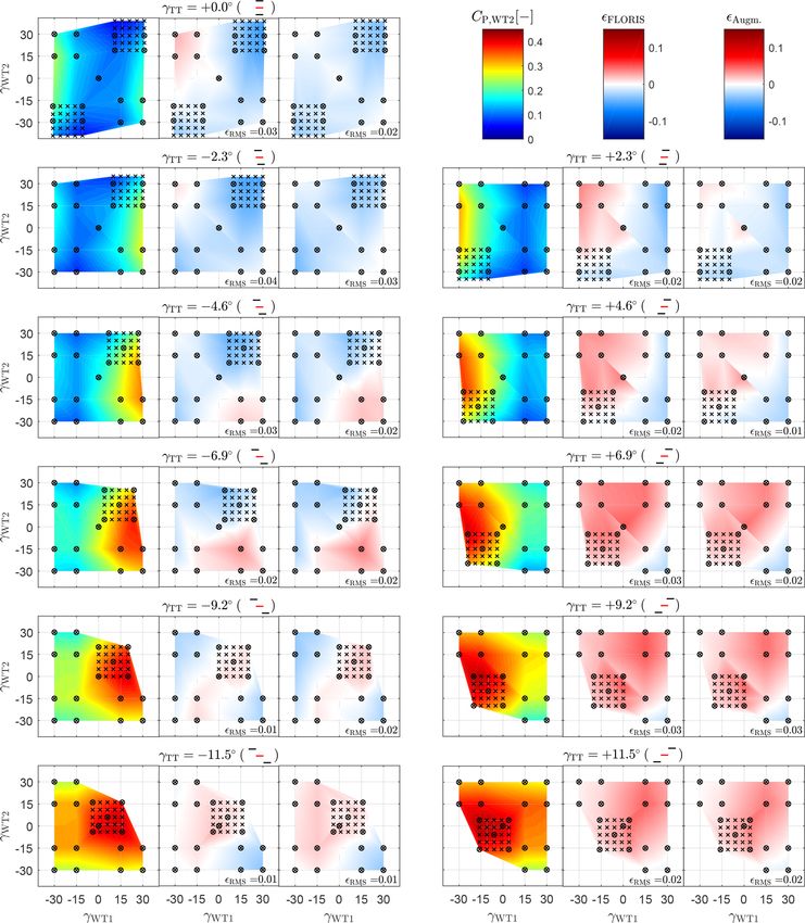
648                                                                          J. Schreiber et al.: Wind farm model augmentation

freedom and hence a much reduced numerical complexity                only know what is contained in the data set that was used to
(Frandsen et al., 2006; Gebraad et al., 2014; Bastankhah and         build it. Typically, this means that a very significant amount
Porté-Agel, 2016). The present paper uses this last family of        of data is necessary to obtain a model that is sufficiently gen-
methods, although ideas similar to the ones developed here           eral and accurate. Furthermore, the data have to cover the
could also be applicable to higher-fidelity models.                  entire spectrum of operation of the system. This also means
   Even though engineering models are constantly improved            that the model might have very poor knowledge (and hence
and refined (Fleming et al., 2018), they will most likely al-        poor performance) for rare situations or conditions that take
ways exhibit only a limited accuracy in many practical ap-           place at the boundaries of the operating envelope, where few
plications, for example whenever an important role is played         if any data points might be available.
by effects such as orography, (seasonal) vegetation, spatial            An alternative to the purely data-driven approach is pre-
variability of the wind, sea state roughness, the erection of        sented in this work, where a reference baseline model is aug-
other neighboring wind turbines, the presence of obstacles,          mented with parametric error terms, which are then identified
and others. In addition, low-fidelity models often lack some         using data. The baseline model already includes prior knowl-
physics, e.g. the flow acceleration caused by wake and rotor         edge based on physics, empirical observations, and experi-
blockage, secondary steering, or others. The idea pursued in         ence. Therefore, even prior to the use of data, a minimum per-
this paper is then to take a rather pragmatic approach: based        formance can be guaranteed. The model is augmented with
on the realization that it will always be difficult – if not alto-   parametric error terms, whose choice is driven by physics
gether impossible – to include all effects and all physics in a      and the knowledge of the limitations of the baseline model.
model of limited numerical complexity, a given model is cor-         Once the errors are identified using operational data, their in-
rected by unknown parametric terms, which are then learned           spection can clarify the causes of discrepancy between model
by using operational data.                                           and measurements. Eventually, this can be used to improve
   The idea of improving an existing model based on mea-             the underlying baseline model. Furthermore, by looking at
surements is hardly new, and it is actually an important topic       the magnitude of the identified errors, significant deviations
in the areas of controls and system identification. For exam-        from the baseline model can be flagged to highlight issues
ple, in the field of wind farm flows, a Kalman filtering ap-         with the model itself, the data, or the training process.
proach has been proposed by Doekemeijer et al. (2017) to                Finally, it should be noted that the identification of the er-
update model predictions based on lidar measurements. Here           ror terms can be combined with the tuning of the parameters
again the present paper takes a more pragmatic approach, and         of the baseline model. This addresses yet another problem:
model updating is based exclusively on data provided by the          tuning the parameters of a model that lacks some physics
standard supervisory control and data acquisition (SCADA)            may lead to unreasonable values for the parameters, as the
systems that are typically available on contemporary wind            model is “stretched” to represent phenomena that it does not
turbines. On the one hand this has the advantage that the pro-       contain. By the proposed hybrid approach, the simultaneous
posed method is applicable to existing assets, as it does not        identification of the parameters of the baseline model to-
necessitate extra sensors. On the other hand, given that stored      gether with the ones of the error terms eases this problem,
SCADA data typically represent 10 min averages, this also            as unmodeled phenomena can be captured by the model-
implies that the models obtained by this technique are of a          augmenting terms, thereby reducing the chances of nonphys-
steady-state nature. Although unsteady effects in wind farms         ical tuning of the baseline parameters.
are clearly important, steady-state models are still very valu-         The baseline model parameters and the extra correction
able and can support many of the applications listed above. In       terms have a different functional form in the augmented gov-
addition, nothing prevents the generalization of the proposed        erning equations. Hence, they should be distinguishable from
approach to unsteady flow models, assuming that the relevant         each other, as they imply different effects on the model. How-
higher-frequency data sets are available, which is already the       ever, as for many identification problems, it is in general not
subject of ongoing work from these authors.                          possible to guarantee that all unknown parameters are ob-
   The contemporary literature – and not only in the field of        servable and noncollinear given a set of measurements and,
wind energy – indicates an increasing interest in data-driven        hence, given a certain informational content. To address this
approaches. Just to give one single example related to wake          problem, the method proposed by Bottasso et al. (2014a) is
modeling, a purely data-driven approach has been recently            used here, where the original unknown parameters are recast
described by Göçmen and Giebel (2018). However, the cur-             into a new set of statistically uncorrelated variables by using
rent enthusiasm for data should not make one forget that             the singular value decomposition (SVD) of the inverse Fisher
physics-based and analytical models are also extremely valu-         information matrix. Once the problem has been solved in the
able because they often encapsulate significant knowledge on         space of the orthogonal uncorrelated parameters, the solution
a given problem, often corroborated by long experience. In           is mapped back onto the original physical space. This ap-
fact, purely data-driven approaches suffer from a number of          proach not only avoids the ill-posedness of the original prob-
limitations that descend directly from a very simple and in-         lem, but also allows one to clarify which physical parameters
evitable fact: a model that is exclusively based on data can         are visible given a certain data set.

Wind Energ. Sci., 5, 647–673, 2020                                                       https://doi.org/10.5194/wes-5-647-2020
J. Schreiber et al.: Wind farm model augmentation                                                                                  649

    The paper is organized as follows. First, the baseline            is repeated marching downstream throughout the wind farm
model is introduced in Sect. 2.1, together with a detailed de-        until the last downstream turbine is reached.
scription of the proposed parametric corrections in Sect. 2.2.           In this work, the implementation uses the selfSimilar
Next, the SVD-based parameter identification method is pre-           FLORIS velocity deficit model, the rans deflection model,
sented in Sect. 2.3. The approach is then applied in Sect. 3.1        the quadraticRotorVelocity wake combination model, and
to a cluster of scaled wind turbines operating in the atmo-           the crespoHernandez added turbulence model. The interested
spheric test section of the wind tunnel of the Politecnico di         reader is referred to Bastankhah and Porté-Agel (2016), Cre-
Milano (Bottasso et al., 2014b). The goal of this first applica-      spo and Hernández (1996), and Doekemeijer et al. (2019)
tion is to show that a correct identification of the error terms      and references therein for detailed descriptions and deriva-
can be achieved. This is indeed possible in the controllable          tions of these models.
and repeatable conditions of a wind tunnel, where inflow and             Engineering wake models depend on a number of param-
wake characteristics can be precisely measured, something             eters, which should be tuned in order to obtain accurate pre-
that is hardly possible today in the field. Specifically, it is       dictions. For the specific model used in this work, these tun-
shown that the method can correctly learn the lack of unifor-         able factors are the wake parameters α, β, ka , kb , ad , and bd
mity of the wind tunnel inflow, which is akin to what happens         and the turbulence model parameters TIa , TIb , TIc , and TId
in a real wind farm because of orographic effects. Similarly,         (Bastankhah and Porté-Agel, 2016).
it is shown that secondary steering, which is completely ab-             In this work, the parameters are first set to an initial value,
sent from the baseline model used here, can be learned by us-         either taken from the literature or identified with ad hoc mea-
ing turbine power measurements only. A more extended view             surements; these initial values are held fixed throughout the
on the wind tunnel results is reported in Appendix A. After           analysis and not changed further. Corrections to the initial
having demonstrated the method in the known and controlled            values are then expressed as
wind tunnel environment, a second application is developed
in Sect. 3.2 that targets a real 43-turbine wind farm. Here re-       k = k ∗ + pk ,                                                (1)
sults indicate that the augmented model has a markedly im-            where k is a model parameter, k ∗ its initial value, and pk
proved prediction capability when compared to the baseline            the correction. Although this is not strictly necessary, this re-
one, thanks primarily to the identification of orographic ef-         dundant notation helps highlight the changes to the nominal
fects on the inflow and the tuning of other model parameters.         model parameters obtained by the proposed procedure.
Finally, conclusions are drawn in Sect. 4.
                                                                      2.2   Model augmentation

2     Methods                                                         The engineering model described earlier is a rather simple
                                                                      approximation of a flow through a wind power plant and it
2.1    Baseline wind farm flow model                                  is therefore bound to have only a limited fidelity to reality,
                                                                      with a consequently only limited predictive accuracy. Even
The proposed method is applied here to the baseline wake              for more sophisticated future models, it is difficult to imag-
model of Bastankhah and Porté-Agel (2016), implemented                ine that all relevant physics will ever be precisely accounted
within the FLORIS framework (Doekemeijer and Storm,                   for. But even if such a model existed, in practice one might
2018). Given ambient wind conditions, steady-state veloc-             simply not have all necessary detailed information on the rel-
ities within a wind farm can be computed by this model,               evant boundary and operating conditions that would be re-
together with the corresponding operating states and power            quired. For example, one might not know with precision the
outputs of all its turbines. First, ambient conditions are es-        conditions of the vegetation around and within a wind farm,
timated from un-waked machines operating in free stream,              with its effects on roughness and, hence, on the flow charac-
which are identified by the turbine yaw orientations and the          teristics. In other words, it is safe to assume that all models
wake model (Schreiber et al., 2018). Then, power and thrust           are in error to some extent and probably always will be.
of the upstream turbines are computed based on the turbine               To address this problem, the model can be pragmatically
aerodynamic characteristics, regulation strategy, and align-          augmented with correction terms. Here one could take two
ment with the local wind direction. Next, the wakes shed by           alternative approaches: either a generic all-encompassing er-
these turbines are calculated in terms of their trajectory and        ror term is added to the model or “surgical” errors are intro-
speed deficit. In turn, this yields the velocity at the rotor disks   duced at ad hoc locations in the model to target specific pre-
of the turbines immediately downstream. In the case of mul-           sumed deficiencies. The first approach could be treated with
tiple wake impingements on a rotor, a combination model               a brute-force parametric modeling approach, for example by
is used to superimpose multiple wake deficits. Similarly, an          using a neural network. Here, the second approach was used,
added turbulence model is used to estimate the turbulence in-         as it allows for more insight into the nature of the identified
tensity at a downstream turbine rotor disk, as this local ambi-       corrections. The specific parametric corrections used in the
ent parameter affects the expansion of the wake. This process         present paper are reviewed next. It is clear that these are only

https://doi.org/10.5194/wes-5-647-2020                                                         Wind Energ. Sci., 5, 647–673, 2020
650                                                                         J. Schreiber et al.: Wind farm model augmentation

some of the many corrections that could be applied to the                Local orographic effects and blockage may also induce
present baseline model, so that the following does not pre-              variability in the wind direction 0. Similarly, the verti-
tend to be a comprehensive treatment of the topic. Nonethe-              cal shear exponent αvs and turbulence intensity I may
less, results indicate that some of these corrections are in-            vary, for example on account of nonuniform roughness
deed significant and provide for a marked improvement of                 induced by vegetation or other obstacles. To include
the baseline model.                                                      these effects in the farm flow model, the baseline quan-
                                                                         tities are augmented as
  – Nonuniform inflow. The inflow to a wind farm can ex-
    hibit spatial variability, mostly because of orographic              0(Y ) = 0ref + Y faugm,dir 0ref , cdir , pdir ,      (3a)
    and local effects, especially in complex terrain condi-

                                                                         αvs (0) = αvs,ref + faugm,shear 0, cshear , pshear , (3b)
    tions. For example, commercial wind resource assess-
                                                                         I (0) = Iref + faugm,I 0, cI , pI .                  (3c)
    ment tools include topographic speedup ratios custom-
    arily computed by CFD models (Jacobsen, 2019). In                    In all these expressions, (·)ref indicates a baseline
    contrast to this established practice, no direct or equiv-           reference quantity, while function faugm,(·) is a cor-
    alent modeling of orographic effects is at present avail-            rection term. This function is defined on the 1D
    able in engineering wake models. Another reason for                  space 0 ∈ [0min , 0max ], discretized with nodes c(·) =
    inflow variability may be due to wind farm blockage ef-              [. . .; 0i ; . . .](·) , using linear shape functions to interpo-
    fects (Bleeg et al., 2018). Indeed, current wake models              late the corresponding nodal values p(·) . Here again, by
    such as the one used here assume that upstream turbines              selecting 0min and 0max , corrections can be applied to
    affect downstream ones through their wakes but do not                the whole wind rose or just to a sector.
    model the effects of downstream machines on the up-
    stream ones. In a wind farm, depending on the wind di-             – Secondary steering. By misaligning a wind turbine ro-
    rection and cross-wind location considered, the number               tor with respect to the incoming flow direction, the ro-
    and operating state of downstream turbines vary, which               tor thrust force is tilted, thereby generating a cross-flow
    may induce a cross-wind speed variability in the inflow.             force that laterally deflects the wake. As shown with the
                                                                         help of numerical simulations by Fleming et al. (2018),
      To capture some of these effects, the model ambient                this cross-flow force induces two counter-rotating vor-
      flow speed V∞ is expressed here as a function of height            tices that, combining with the wake swirl induced by
      above ground Z, cross-wind lateral position Y , and am-            the rotor torque, lead to a curled wake shape. As ob-
      bient wind direction 0 as                                          served experimentally by Wang et al. (2018), the ef-
      V∞ (Y, Z, 0) =                                                     fects of these vortices result in additional lateral flow
                                                                       speed components, which are not limited to the wake it-
       1 + faugm,speed Y, 0, cspeed , pspeed
            αvs                                                        self but also extend outside of it. By this phenomenon,
             Z                                                           the flow direction within and around a deflected wake
      V∞,0          ,                                           (2)
             zh                                                          is tilted with respect to the upstream undisturbed di-
                                                                         rection. Therefore, when a turbine is operating within
      where V∞,0 is the reference (baseline uncorrected)
                                                                         or close to a deflected wake, its own wake undergoes
      ambient flow speed and zh the reference height of
                                                                         a change of trajectory – termed secondary steering –
      the vertically sheared flow with exponent αvs . Func-
                                                                         induced by the locally modified wind direction. Al-
      tion faugm,speed (Y, 0, cspeed , pspeed ) is the speed correc-
                                                                         though models of this phenomenon are being devel-
      tion term. This function is defined in the 2D space
                                                                         oped (Martínez-Tossas et al., 2019), they significantly
      Y ∈ [Ymin , Ymax ], 0 ∈ [0min , 0max ]. For each value of
                                                                         increase the computational cost and are not yet avail-
      the ambient wind direction 0, Y is a lateral coor-
                                                                         able in standard implementations of engineering wake
      dinate orthogonal to it that spans the width of the
                                                                         models such as the one used here.
      farm; hence, by selecting 0min and 0max a lateral in-
      flow nonuniformity can be modeled for a given sec-                 The change of wind direction 10 at a downstream tur-
      tor or the whole wind rose of directions. The (Y, 0)               bine induced by secondary steering (indicated by the
      space is discretized into rectangular cells with corner            subscript ss) is modeled here as
      nodes cspeed = [. . .; (Yi , 0i ); . . .] (for an example, see
                                                                         10(y) = faugm,ss ỹ, 0init , pss ,               (4)
      Fig. 16). The corresponding unknown error nodal values
      are stored in vector pspeed , and bilinear shape functions         where faugm,ss is the correction term and ỹ = Y − ywc is
      interpolate the error in each cell based on the nodal val-         the lateral distance to the wake centerline (see Fig. 1),
      ues at its corners. Equation (2) could be extended to also         defined in the baseline wind farm model as the locus
      include a longitudinal wind-aligned coordinate, simi-              of the points of minimum flow speed. According to the
      larly to the localized speedup ratios of Jacobsen (2019),          notation used in Eq. (6.12) of Bastankhah and Porté-
      to model wind farm blockage effects.                               Agel (2016), 0init indicates the initial wake direction of

Wind Energ. Sci., 5, 647–673, 2020                                                       https://doi.org/10.5194/wes-5-647-2020
J. Schreiber et al.: Wind farm model augmentation                                                                                  651

    the closest upstream turbine. The correction term is ex-                of the speed deficit within the wake. Another assump-
    pressed as the difference of two Gaussian functions and                 tion is that the flow outside the wake is undisturbed and
    more precisely                                                          equal to the free stream. However, these assumptions
                                                                           can, at times, not be exactly satisfied, as already ob-
    faugm,ss ỹ, 0init , pss =                                              served by Xie and Archer (2017) and Martínez-Tossas
                                                      !
                                 ỹ + sgn(0init )pss,3 2                    et al. (2019), among others. For example, aisle jets are
    0init pss,1 exp −0.5                                                    local accelerations of the flow outside of the wake, pro-
                                         pss,2
                                                                            duced by local blocking in the neighborhood of an oper-
                                                   !!
                            ỹ + sgn(0init )pss,6 2                         ating turbine. It has been reported that aisle jets can in-

     −pss,4 exp −0.5                                     , (5)              duce local flow speedups in excess of 10 % of the undis-
                                     pss,5
                                                                            turbed inflow (Dörenkämper et al., 2015).
    where pss = (pss,1 , pss,2 , pss,3 , pss,4 , pss,5 , pss,6 ) is the     To account for such effects, the wake velocity Vwake of
    vector of free parameters, where parameters 1 and 4 are                 the baseline model is corrected as
    related to the amplitude, 3 and 6 to the standard devia-
    tion, and 2 and 5 to the location of the correction func-               Vwake (dwc ) =

    tions. Since the Gaussian functions are not centered at                 Vwake,FLORIS (dwc ) 1 + faugm,acc dwc , cacc , pacc , (6)
    the wake centerline and the effect of secondary steer-
    ing is assumed to be symmetric with respect to the mis-                 where Vwake,FLORIS is the baseline Gaussian wake speed
    alignment angle, the correction term also depends on the                profile, dwc is the absolute distance to the wake center
    direction of wake deflection sgn(0init ).                               (which, at hub height, is equivalent to |ỹ|), and faugm,acc
    This particular choice of the shape functions is moti-                  represents the correction term, which – similarly to the
    vated by the results shown in Fig. 8b of Wang et al.                    previous corrections – is modeled with linear shape
    (2018). Indeed, LES simulations and measurements re-                    functions characterized by node locations cacc (in terms
    veal the presence of a stronger lateral velocity compo-                 of dwc ) and nodal values pacc .
    nent directed towards the wake on the leeward side of
                                                                          – Reduced power extraction due to nonuniform wind tur-
    the wake itself, and of an opposite and weaker lateral
                                                                            bine inflow. Numerical simulations conducted in FAST
    component on the windward side. Such a distribution
                                                                            (Jonkman and Jonkman, 2018) using its blade element
    can be approximated by two Gaussian functions using
                                                                            momentum (BEM) implementation yielded a slight re-
    Eq. (5).
                                                                            duction in the rotor power coefficient for horizontally
    Note that the change in local wind direction also leads to              sheared flow, when compared to unsheared conditions
    a slight lateral deflection of the nonuniform wind farm                 with the same hub wind speed. Even though BEM can
    inflow introduced previously. More precisely, for a tur-                only give a rough indication for such an effect, a cor-
    bine that is located 1X behind an upstream turbine, the                 rection of the power coefficient of the baseline model is
    nonuniform inflow expressed by Eq. (2) is evaluated at                  introduced here in the form
    Y + 1X sin(10) instead of Y .
    Figure 1a shows the hub height flow speed for two                       CP = CP,κ=0 1 + pκ κ 2 ,                             (7)
    wind turbines modeled in FLORIS, with the turbine ro-
    tor disks being indicated with thick black lines. The                   where CP,κ=0 is the nominal power coefficient, κ the
    wake centerlines and the undisturbed free-stream wind                   equivalent horizontal linear shear coefficient on the ro-
    direction are indicated by black dotted and dashed lines,               tor disk, and pκ the free correction parameter. The lin-
    respectively. The upstream turbine is misaligned with                   ear shear κ is either due to a lack of lateral uniformity
    respect to the incoming flow, and therefore its wake                    of the inflow or due to the impingement of a wake, and
    is deflected laterally. Using the baseline wake model,                  it is evaluated accordingly within the farm model.
    the downstream turbine wake develops along the free-
    stream wind direction. Panel (b) of the same figure                   – Wind-speed-dependent power loss in yaw misalignment.
    shows the effects of the secondary steering correction                  The baseline formulation models the power extraction
    term given by Eq. (5). The plot clearly shows that the                  of a misaligned wind turbine using the cosine law
    downstream turbine wake path is affected by the locally                 CP (γ ) = CP cos(γ )pP , where CP is the power coefficient
    changed wind direction.                                                 of the wind-aligned turbine, γ the misalignment an-
                                                                            gle with respect to the local flow direction, and pP the
  – Non-Gaussian wake and flow acceleration. Engineering                    power loss exponent. Different power loss exponents
    wake models are based, among other hypotheses, on                       have been reported in the literature, ranging from the
    assumed shapes of the speed deficit. For example, the                   value of 1.4 found by Fleming et al. (2017) to 1.8 ac-
    present baseline model assumes a Gaussian distribution                  cording to Schreiber et al. (2017), 1.9 for Gebraad et al.

https://doi.org/10.5194/wes-5-647-2020                                                         Wind Energ. Sci., 5, 647–673, 2020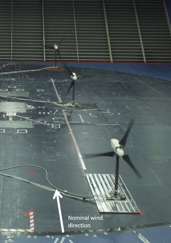
652                                                                           J. Schreiber et al.: Wind farm model augmentation

                                                                      changes in the parameters. For example, a flat maximum of
                                                                      the function implies that different nearby values of the model
                                                                      parameters are associated with similar values of the likeli-
                                                                      hood. These characteristics of the solution space are captured
                                                                      by the Fisher information matrix, which can be interpreted
                                                                      as a measure of the curvature of the likelihood function. Fur-
                                                                      thermore, it can be shown that the variance of the estimates is
                                                                      bound from below (Cramér–Rao bound) by the inverse of the
                                                                      Fisher matrix (Jategaonkar, 2015). Although the analysis of
                                                                      the Fisher information is useful for the understanding of the
                                                                      well-posedness of an estimation problem and of the quality
                                                                      of the identified model, it does not offer a constructive way of
Figure 1. Effect of secondary steering on the trajectory of a down-   reformulating a given ill-posed problem. Indeed, a flat solu-
stream turbine. (a) Baseline wake model; (b) baseline model aug-      tion space and collinear parameters are to be expected in the
mented with the empirical correction term of Eq. (5).                 present case, given the complex couplings and dependencies
                                                                      that may exist among the various parameters of a wind farm
                                                                      flow model and its correction terms.
      (2015), and all the way to the ideal value of 3 that is ex-         To overcome this limitation of the classical maximum like-
      pected if only the rotor-orthogonal ambient flow com-           lihood formulation, following Bottasso et al. (2014a), the
      ponent contributes to power extraction (Boersma et al.,         original physical parameters of the model are transformed
      2019). In addition, pP might also depend on the regu-           into an orthogonal parameter space, by diagonalizing the
      lation strategy used by the turbine controller. Here, the       Fisher matrix using the SVD. This way, as the parameters are
      power coefficient in misaligned operation is augmented          now statistically decoupled, one can set a lower observabil-
      as                                                              ity threshold and in the analysis retain only the ones that are
      CP = CP cos (γ + pP0 )pP +pP,a (V −Vrated )+pP,b ,       (8)    in fact observable given the available set of measurements.
                                                                      Once the problem is solved, the uncorrelated parameters are
      where CP is the power coefficient of the flow-aligned           mapped back onto the original physical space.
      turbine (possibly reduced by shear effects, as argued               As shown later on, this approach achieves multiple goals:
      above), pP0 is the misalignment angle at which the tur-         it allows one to successfully solve a maximization problem
      bine produces maximum power, and V and Vrated are,              with many free parameters, some of which might be interde-
      respectively, the rotor effective and rated wind speeds.        pendent on one another or not observable in a given data set;
      Finally, pP is the baseline exponent, while pP,a and pP,b       it reduces the problem size, retaining only the orthogonal pa-
      are free parameters that model a linear wind speed de-          rameters that are indeed observable; it highlights, through the
      pendency of the cosine law.                                     singular vectors, the interdependencies that may exist among
                                                                      some parameters of the model, which provides for a useful
                                                                      interpretation tool that may guide the reformulation of parts
2.3   Parameter identification method
                                                                      of the model and its correction terms.
The parameters of the baseline model and of its correction
terms are identified with the method developed by Bottasso            2.3.1   Maximum likelihood estimation of model
et al. (2014a). The formulation of the parameter estimation                   parameters
problem is independent of whether the parameters belong to
the baseline model or to its correction factors. In this sense,       A steady-state wind farm model can be mathematically ex-
one can use the same method to just tune the baseline param-          pressed as
eters without considering the correction terms, just identify         y = f (p, u),                                               (9)
the correction terms at the frozen baseline model, or concur-
rently identify both sets.                                            where f (·, ·, ·) is the nonlinear static function describing
   The formulation is based on the classical likelihood func-         the wind farm model, which depends on free parameters
tion, which describes the probability that a given set of noisy       p ∈ Rn . These parameters can include both wake model pa-
observations can be explained by a specific set of model pa-          rameters and/or model augmentation parameters. The model
rameters. By numerically maximizing this function, a set of           inputs u ∈ Rnu include ambient wind conditions (i.e. ambi-
parameters is identified that most probably explains the mea-         ent wind speed, direction, air density, turbulence intensity)
surements. Bound constraints are used to guide the process            and control inputs (i.e. yaw misalignment, partialization fac-
and ensure convergence to meaningful results.                         tor, blade pitch, rotor speed of each turbine). The model out-
   The accuracy with which the parameters can be estimated            puts y ∈ Rm represent quantities of interest for which mea-
depends on how flat the likelihood function is with respect to        surements are available, in the present work these being the

Wind Energ. Sci., 5, 647–673, 2020                                                        https://doi.org/10.5194/wes-5-647-2020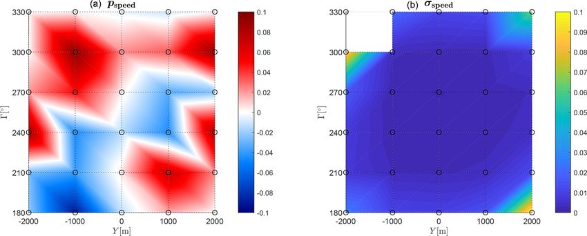
J. Schreiber et al.: Wind farm model augmentation 653
power outputs of each wind turbine in the farm. Experimen- 2.3.2 Identifiability of parameters
tal observations z of the simulated outputs y will in general
result in a residual r ∈ Rm , caused by measurement and pro- The Fisher information matrix F ∈ Rn×n is defined as
cess noise (e.g. plant–model mismatch), so that N
∂y i T
X ∂y i
F= R−1 (15)
z = y + r. (10) i=1
∂p ∂p
Given a set S = {z1 , z2 , . . ., zN } of N independent obser- and describes the curvature of the likelihood function. It can
vations, the likelihood function (Jategaonkar, 2015) can be be shown (Jategaonkar, 2015) that a lower bound (termed
defined as Cramér–Rao bound) of the covariance of the estimated pa-
rameter is given by
N
Y
L(S p ) = p zi p , (11) F−1 = P ≤ Var pMLE − ptrue ,
(16)
i=1
where ptrue represents the true but unknown parameters. The
where p(·) is the probability of S given p. Assuming the
kth diagonal element of P is a lower bound on the variance
residuals r with covariance R to be statistically independent
of the kth estimated parameter, while the correlation between
within the set of measurements (i.e. E[r i r Tj ] = R δi,j , where
different parameters is captured by the off-diagonal terms of
δi,j is the Kronecker delta), the likelihood function can be
that same matrix. The correlation coefficient between two pa-
written, following Jategaonkar (2015), as
rameters i and j is defined as
L Sp = Pi,j
9pi ,pj = p , (17)
N
! Pi,i Pj,j
−N/2 1X
(2π)m det R−1 exp − r T Rr i . (12)
2 i=1 i where Pi,j denotes the i, j th element (row, column) of P.
By analyzing the estimated parameter variance, as well as
Maximizing L (or minimizing its negative logarithm), a max- the correlation between parameters, valuable insight into the
imum likelihood estimate of the parameters can be obtained well-posedness of the parameter identification problem can
as be readily obtained.
pMLE = argminJ (p), (13)
p 2.3.3 Problem transformation and untangling using the
SVD
where J (p) = − ln(L(S p ). The measurement noise covari-
ance Pmatrix R can be estimated under mild hypotheses as When some parameters are highly correlated or have large
R= N T variance, the problem is ill-posed: it might exhibit sluggish
i=1 r i r i , yielding J (p) = det(R), leading to an itera-
tion between a solution at given covariance and a covariance convergence, or no convergence at all, and small changes in
update step (Jategaonkar, 2015). However, in this paper the the inputs may lead to large changes in the estimates. Such
measurement noise covariance matrix is estimated a priori situations are difficult to solve in physical space, because
and therefore assumed to be known. The cost function there- parameters are typically coupled together to some degree
fore becomes through the model.
To untangle the parameters, one may resort to the SVD
N (Golub and van Loan, 2013). By this approach (Hansen,
1X
J (p) = r T R−1 r i . (14) 1987; Waiboer, 2007; Bottasso et al., 2014a), the original pa-
2 i=1 i
rameters are mapped into a new set of uncorrelated (orthog-
onal) parameters. Since the new unknowns are uncorrelated,
To ensure reasonable and physically viable solutions, pa-
one can set a threshold to their variance by using the Cramér–
rameters can be forced to stay within predefined upper (sub-
Rao bound and only retain those in the optimization that are
script ub) and lower (subscript lb) bounds, by adding the
observable within the given data set.
corresponding inequality constraints plb ≤ p ≤ pub to prob-
The Fisher matrix F is first factorized as F = MT M, where
lem (13). As the parameter values and constraints can differ
M ∈ RNm×n is defined as
in magnitude, it is a good practice to scale all parameters
such that a value of 1 corresponds to the upper bound pub −1/2 ∂y 1
R ∂p
and a value of −1 to the lower one plb . The optimization −1/2 ∂y 2
problem can finally be solved numerically by a suitable al- R ∂p
M= . (18)
gorithm, such as sequential quadratic programming (SQP) ...
∂y
(Nocedal and Wright, 2006). R−1/2 ∂pN
https://doi.org/10.5194/wes-5-647-2020 Wind Energ. Sci., 5, 647–673, 2020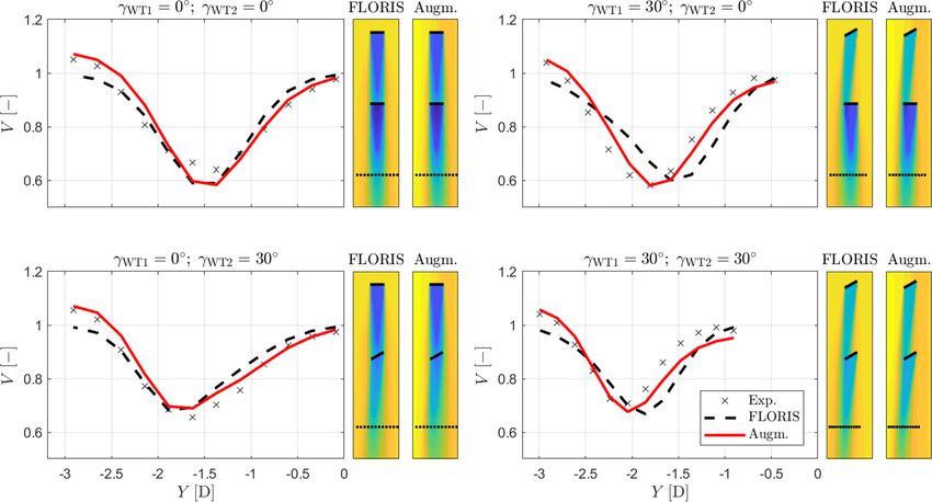
654 J. Schreiber et al.: Wind farm model augmentation
Assuming a larger number of measurements than parameters 2.3.4 Identification method with variable measurement
(Nm > n), matrix M can be decomposed into weights
M = U6VT , (19) In some cases, it may be useful to increase the importance
of some measurements in the parameter estimation problem.
where U ∈ RNm×Nm and V ∈ Rn×n are the matrices of left This can be readily obtained by simply treating an observa-
and right, respectively, singular vectors, while tion with weight w as if it appeared w times in the obser-
vation data set (Karampatziakis and Langford, 2011). Cost
function (14) then becomes
S
6= , (20)
0 N
1X
J (p) = wi r Ti R−1 r i , (25)
where S ∈ Rn×n is a diagonal matrix, whose entries si are the 2 i=1
singular values sorted in descending order.
By using Eq. (19) and the factorization of F, the inverse of where
PN wi is the relative weight of observation i and
the Fisher information matrix can be written as i=1 wi = N. Similarly, the Fisher matrix becomes
P = VS−2 VT . N T
(21)
X ∂y i ∂y i
F= wi R−1 , (26)
i=1
∂p ∂p
Note that the columns of the orthogonal matrix V are also
the eigenvectors of P and si−2 the corresponding eigenval- and its factorization is
ues. Furthermore, P and F are symmetric and, based on the √ ∂y
spectral theorem, diagonalizable. w1 R−1/2 ∂p1
The physical parameters p can now be transformed into a √ ∂y
w2 R−1/2 ∂p2
new set of orthogonal parameters 2 by a rotation performed M= . (27)
...
with the right singular values: √ −1/2 ∂y N
wN R ∂p
2 = VT p. (22)
The remainder of the formulation is not affected by the intro-
For the transformed set of parameters, the Cramér–Rao duction of weights.
bound on the variance of the estimates is the diagonal matrix
S−2 ≤ Var(2MLE − 2true ). Therefore, a small singular value 3 Results
si corresponds to a large uncertainty in the corresponding or-
thogonal parameter estimation. The proposed method is first applied in Sect. 3.1 to a wind
To remove parameters that cannot be estimated with suffi- tunnel experiment with a small cluster of three wind tur-
cient accuracy, matrix S can be partitioned as bines and then in Sect. 3.2 to a real wind farm consisting
of 43 wind turbines. The former example aims at a verifica-
SID 0 tion of the correctness of the identified augmentations, given
S= , (23)
0 SNID the known and controllable conditions of the scaled experi-
ments, whereas the latter is meant to offer a first glimpse of
where SID contains the identifiable singular values, i.e. those the practical applicability of the new method in the field.
such that si−2 < σt2 , σt being a threshold on the highest ac-
ceptable standard deviation in the estimate. On the other 3.1 Wind tunnel verification
hand, matrix SNID contains singular values associated with
parameters that cannot be identified with sufficient accuracy Whether identified model corrections are indeed physical or
and are therefore discarded. Accordingly, V is also parti- only an artifact of the model–measurement mismatch is diffi-
tioned as V = [VID , VNID ], while the orthogonal parameters cult to prove in general. From this point of view, wind tunnel
are partitioned as 2 = [2TID , 2TNID ]T . Finally, the physical experiments provide a unique opportunity to verify the con-
parameters are expressed in terms of the sole identifiable or- cept proposed in this paper. Indeed, the overall flow within a
thogonal parameters: cluster of turbines can be measured with good accuracy, and
the experiments can be repeated in multiple desired operat-
p ≈ VID 2ID . (24) ing conditions. The aim of this section is then to show that,
even in the presence of multiple possibly overlapping model
Given that the Fisher matrix depends on the values of the pa- terms, the correct improvements to a baseline model can be
rameters p, an iterative procedure should be followed, where learned from operational data only.
the diagonalization of the problem is repeated at each update
of the parameter vector.
Wind Energ. Sci., 5, 647–673, 2020 https://doi.org/10.5194/wes-5-647-2020
J. Schreiber et al.: Wind farm model augmentation                                                                                   655

Figure 2. Wind farm layout for a null turntable rotation, looking
down onto the wind tunnel floor.

3.1.1   Experimental setup
                                                                     Figure 3. View looking downstream of the cluster of three G1 tur-
                                                                     bines.
The experimental setup is composed of a scaled cluster of
three G1 wind turbines, each of them equipped with active
yaw, pitch, and torque control. The turbines were operated           fore not placed on the turntable, and its position remained
in the boundary layer test section of the wind tunnel of the         fixed with respect to the wind tunnel test section. A wind-
Politecnico di Milano. Details on the models and the wind            tunnel-fixed reference frame, used in the following to discuss
tunnel are reported, among other publications, in Campag-            the results, is also depicted in Fig. 2. Its origin is placed at the
nolo et al. (2016a, b, c).                                           turntable center, while the frame x axis is aligned with the
   The turbines are labeled WT1, WT2, and WT3, starting              wind direction; the y axis points left, looking downstream;
from the most upstream one and moving downstream. The                and hence Z points vertically up from the floor to complete
machines are mounted on a turntable, whose rotation is used          a right-handed triad.
to change the wind direction with respect to the wind farm              The yaw angle γWTi of the ith wind turbine is positive for
layout. In the nominal configuration, i.e. for a turntable ro-       a counterclockwise rotation looking down onto the floor, as
tation γTT = 0◦ , the three turbines are aligned with the wind       shown for WT1 in Fig. 2, and null when the rotor disk is or-
tunnel main axis – and hence with the flow velocity vector.          thogonal to X and, therefore, to the nominal wind direction.
The turbines are installed with a longitudinal spacing of 5             Figure 3 shows a photo of the cluster of turbines, looking
diameters (D), as shown in Fig. 2 with a view looking down           downstream with WT1 in the foreground. The wind tunnel
towards the wind tunnel floor. As indicated in the figure, pos-      floor is blue, whereas the turntable is black.
itive turntable rotations are clockwise. For γTT 6 = 0◦ , the lon-      The ambient wind speed V∞,0 measured by the pitot
gitudinal distance between the turbines decreases slightly.          tube was, for all conducted experiments, between 5.20 and
However, considering that in this work the largest investi-          5.75 m s−1 , which corresponds to slightly below-rated condi-
gated turntable angle was ±11.5◦ , the longitudinal distance         tions. The ambient turbulence intensity was equal to 6.12 %,
varied only between 4.9D and 5D.                                     while the vertical shear was αvs = 0.144.
   A pitot probe was placed at hub height, 3D upstream of the
first G1 in the nominal configuration. The probe was there-

https://doi.org/10.5194/wes-5-647-2020                                                        Wind Energ. Sci., 5, 647–673, 2020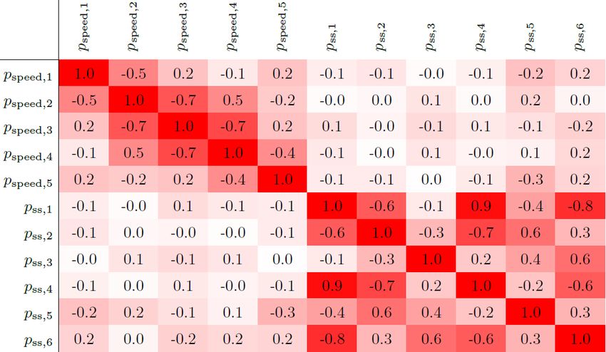
656                                                                         J. Schreiber et al.: Wind farm model augmentation

                                                                    disk area. Here, power was computed    by integrating over the
                                                                    rotor disk area, i.e. P = 1/2ρ A V 3 CP dA, which is probably
                                                                                                  R

                                                                    slightly more accurate even though it involves a minor in-
                                                                    crease in computational effort.

                                                                    3.1.3   Ranking of correction terms

                                                                    To initially assess the role of the various parameters, a rank-
                                                                    ing analysis was conducted. The parameters were clustered
                                                                    in sets, depending on their role in the model. A first identi-
                                                                    fication was performed using all parameter sets, yielding the
                                                                    presumed best value, denoted Jref , of the cost function ex-
                                                                    pressed by Eq. (14). The analysis was then repeated multiple
                                                                    times, each time removing one parameter set from the opti-
                                                                    mization. By looking at the resulting change in the value of
                                                                    the cost function, one may then rank the various parameter
                                                                    sets in order of importance. The analysis is based on a to-
Figure 4. Power and thrust coefficients vs. wind speed for the G1   tal of 190 experimental observations, as described in greater
turbine.                                                            detail in the following.
                                                                       All augmentation terms described in Sect. 2.2 were con-
                                                                    sidered, except for the lateral variation in wind direction
3.1.2      Model setup                                              and the wind-direction-dependent vertical shear, as they are
                                                                    not applicable to the wind tunnel experiments. The nonuni-
The FLORIS model implementation used in this work is                form flow speed was modeled using five nodes located at
the one available online (Doekemeijer and Storm, 2018). All         cspeed (Y ) = [−3, −2, −1, 0, 1] m (which correspond to ap-
baseline model parameters are reported in Table 1 and taken         proximatively [−2.7, −1.8, −0.9, 0, 0.9]D) and also indi-
from Campagnolo et al. (2019), where they were identified           cated in Fig. 2 using × symbols. As only the turbine positions
based on wake measurements of a single isolated G1 turbine.         with respect to the flow are modified by rotating the turntable,
   Figure 4 shows the G1 power CP and thrust CT coefficients        a wind direction dependency was not included in this correc-
as functions of wind speed V . The curves were obtained from        tion term. Table 2 reports the initial values and lower and
dynamic simulations conducted in turbulent inflow, using the        upper bounds – chosen based on an educated guess – for the
same controllers implemented on the scaled models. The CP           nonuniform inflow and secondary steering correction terms.
and CT vs. tip speed ratio (TSR) and blade pitch setting               Figure 5 shows the relative increase in the cost function
curves were obtained with a BEM formulation using experi-           when eliminating one parameter set at a time. The figure
mentally tuned airfoil polars (Bottasso et al., 2014a). As the      clearly indicates that the most important parameters are the
turbine controller does not consider variations in air density      ones modeling laterally nonuniform speed and secondary
ρ, the coefficients shown in the figure exhibit a slight depen-     steering. Indeed, this particular wind tunnel, due to its inter-
dency on this ambient parameter. Within FLORIS, this effect         nal configuration and large width, does present a significant
is taken into account by interpolating within the coefficients      nonuniform flow speed, as already discussed by Campagnolo
based on the actual density measured in the wind tunnel             et al. (2019). Likewise, the effect of secondary steering is par-
during each experiment. For all reported test conditions, air       ticularly important and should not be neglected for accurate
density varied in the range ρ ∈ [1.159, 1.185] kg m−3 . The         predictions in misaligned conditions, as already reported in
power loss exponent in misaligned conditions was evaluated          various publications. Based on these results, in the following
experimentally to be pP = 2.1741, while for thrust the coef-        only nonuniform inflow and secondary steering corrections
ficient was found to be pT = 1.4248.                                are considered.
   The ambient wind speed was determined from the pitot
tube. It was observed that, by using this value, the power of       3.1.4   Results
a free-stream turbine predicted by the FLORIS model was
slightly underestimated, most probably due to the sheared           A total of 451 observations were available, including 11 dif-
flow. To correct for this effect, measurements provided by the      ferent turntable positions and thus wind farm layouts, with
pitot tube were scaled by the factor 1.0176, which was com-         turbine yaw misalignments ranging from −40 to +40◦ . A
puted in order to match simulated and measured power. Fur-          total of 190 observations were used to identify the five pa-
thermore, in the original FLORIS implementation the power           rameters associated with nonuniform inflow speed and the
of a turbine is computed as P = 1/2ρAVavg   3 C , where V           six associated with secondary steering, whereas the remain-
                                                 P          avg
is the average wind speed at the rotor disk and A the rotor         ing data points were used for model validation. The various

Wind Energ. Sci., 5, 647–673, 2020                                                      https://doi.org/10.5194/wes-5-647-2020
J. Schreiber et al.: Wind farm model augmentation 657
Table 1. Initial FLORIS parameters for the G1 turbine.
α∗ β∗ ka∗ kb∗ ad∗ bd∗ TI∗a TI∗b TI∗c TI∗d
0.9523 0.2617 0.0892 0.027 0 0 0.082 0.608 −0.551 −0.2773
Table 2. Definition of the parameters, together with their initial values, lower and upper bounds, and identified values.
i pi plb,i pub,i pinit,i popt,i Implementation
1–5 p speed [−0.1, −0.1, . . . [0.1, 0.1, . . . [0, 0, 0, 0, 0] [0.079, 0.029, . . . faugm,speed (Y, Z, 0, cspeed , pspeed )
−0.1, −0.1, −0.1] 0.1, 0.1, 0.1] −0.051, −0.006, 0] cspeed = [−3, −2, −1, 0, 1] m
6–11 p ss [−3, 0, . . . [3, 1.5, . . . [−0.5, 0.5, . . . [−0.94, 0.63, . . . faugm,ss (ỹ, 0init , pss )
−3, −3, . . . 3, 3, . . . 0.2, −0.25, . . . 0.20, −0.48, . . .
0, −3] 1.5, 3] 0.5, −0.2] 0.73, −0.28]
The threshold of the highest acceptable standard variance
σt2 for the orthogonal parameters was set to 0.01. As the
parameters are scaled within a range of [−1, 1], the thresh-
old corresponds to a relative variance of 2 %. Wind-aligned
operating conditions (i.e. γWT1 = γWT2 = γWT3 = 0◦ ) were
weighted with a factor of 2, to increase their importance in
the parameter estimation process.
The constrained optimization problem (13) was solved in
MATLAB using the fmincon function with the interior-point
algorithm (Mathworks, 2019). As the baseline model with
its initial nominal values (p = pinit ) is far away from the
optimal solution, a first optimization was performed includ-
ing only the inflow correction. Afterwards, three iterations
were conducted including all 11 parameters. At each itera-
tion, a total of eight orthogonal parameters could be iden-
tified within the specified variance threshold. The method
converged very quickly, as the identified parameters and the
Figure 5. Relative increase in the optimization cost function when residual did not change significantly after the first iteration.
eliminating one parameter set at a time. Figure 6a shows the initial variance of all 11 orthogonal
parameters, and panel (b) shows the variance computed af-
ter the first iteration. The horizontal black line indicates the
tested configurations in terms of turbine misalignments and threshold σt2 .
turntable positions are reported in the figures of Appendix A. Interestingly, the 11th orthogonal parameter seems to have
Among all the available measurements gathered at each a very low observability. Table 3 shows the transformation
operating condition, only the steady-state power of the wind matrix VT that links the physical parameters to the orthog-
turbines was utilized, mimicking what could be done at full onal ones (2 = VT p; see Eq. 22). The 11th orthogonal pa-
scale in the field using SCADA data. The model outputs y rameter is almost entirely associated with pspeed,5 , which cor-
(see Eq. 9) are defined as responds to the inflow speed augmentation node at position
Y = 1 m. Indeed, the location of this node is such that it has
only a very marginal effect on the turbine outputs and, hence,
P
1 WT1 a very low observability, as shown later in Fig. 7. The trans-
y= PWT2 , (28)
Pref PWT3 formation matrix reported in Table 3 also shows that the other
two orthogonal parameters with low observability (9 and 10)
where PWTi is the power of the ith wind turbine and Pref = represent secondary steering modes, mainly associated with
37.6W is a reference value used as the scaling factor. Based the second Gaussian function of the correction term.
on experience, a diagonal measurement noise covariance ma- Table 4 presents the correlation matrix 9 (see Eq. 17) and
trix R with all three terms equal to σ 2 = 0.0252 was speci- shows a clear and to be expected dependency among neigh-
fied. boring inflow parameters. Among the secondary steering pa-
https://doi.org/10.5194/wes-5-647-2020 Wind Energ. Sci., 5, 647–673, 2020658 J. Schreiber et al.: Wind farm model augmentation
Figure 6. Variance of the orthogonal parameters before (a) and after (b) the first iteration. The identifiable orthogonal parameters are shown
in red, whereas all others are shown in blue.
Table 3. Transformation matrix VT after the first iteration. Each row corresponds to a different orthogonal parameter.
rameters, strong but less obvious correlations are present, the inflow node at Y = 1 m has a very low – but still finite –
which suggest that a simplification of the assumed correction observability.
term might be possible. The identified secondary steering augmentation term is vi-
Figure 7 shows the identified inflow augmentation func- sualized in Fig. 8. The plot shows the wind direction change
tion. In the picture, whiskers indicate the parameter uncer- 10 as a function of the distance ỹ to the wake centerline for
tainty σi , computed
p based on the Cramér–Rao lower error a turbine misalignment of 20◦ . The gray shaded area shows
bound as σ = diag(P) (see Eq. 16). The same figure also the uncertainty band popt,i ± σi . Consistently with the find-
reports measurements obtained with hot-wire probes in the ings of Wang et al. (2018), the maximum change in wind
empty wind tunnel at three different heights above the floor. direction is found at approximatively 0.3D on the leeward
These measurements, and especially the ones at hub height, side of a deflected wake. The maximum magnitude of sec-
are in good agreement with the estimates provided by the ondary steering in this operating condition is 1.9◦ , which is
proposed method. The figure also reports (with × symbols) again comparable to the results of Wang et al. (2018).
the lateral position of the upstream turbine for the investi- The validity of the augmentation terms, identified as ex-
gated turntable rotations. Noting that all points are shifted plained, was assessed by comparing the results of the simu-
to the left helps explain why the parameter associated with lation model with experimental wake measurements from a
Wind Energ. Sci., 5, 647–673, 2020 https://doi.org/10.5194/wes-5-647-2020J. Schreiber et al.: Wind farm model augmentation 659
Table 4. Correlation coefficients 9 after the first iteration.
Figure 7. Identified nonuniform inflow speed augmentation term Figure 8. Identified wind direction change 10 due to secondary
(solid line) and associated standard deviation (whiskers). Hot-wire steering as a function of distance ỹ to the wake centerline for a
measurements at different heights above the floor are shown in thin turbine misalignment of 20◦ . The gray shaded area shows the un-
solid lines. The upstream turbine (WT1) y position for all investi- certainty band.
gated turntable rotations is shown by × markers placed along the
lower edge of the figure.
also include the points at which the flow was measured with
different test campaign. The setup was identical to the one the probes.
considered here, except for the fact that only the first two up- In the left subplots, the improvements of the augmented
stream wind turbines were installed in the wind tunnel. At model with respect to the baseline FLORIS are exclusively
the downstream distance where the third wind turbine should due to the inflow correction, as the upstream turbine is
have been installed, flow velocity measurements were ob- aligned with the flow and therefore there are no secondary
tained at turbine hub height using hot-wire probes. Figure 9 steering effects. In the right subplots, the upstream turbine
shows wake profiles for the turntable position γTT = 0◦ for is misaligned (γWT1 = 30◦ ) and secondary steering effects
various combinations of turbine yaw misalignments, as indi- are present. Taking into account that model augmentation
cated by the subplot titles. Each subplot is accompanied by was obtained exclusively by turbine power measurements,
two flow visualizations, one based on the baseline FLORIS the improved matching of the wake profiles is remarkable.
model and the other on its augmented version. The figures Still, even with the extra correction terms some small model
https://doi.org/10.5194/wes-5-647-2020 Wind Energ. Sci., 5, 647–673, 2020660 J. Schreiber et al.: Wind farm model augmentation
Figure 9. Wake profiles 5D behind WT2 for various combinations of turbine yaw misalignment. Experimental values are indicated by the
× symbols. Each subplot is accompanied by two flow visualizations based on the FLORIS model and its augmented version.
mismatches are present; these might be caused by the wake
combination model, which was not augmented in this study.
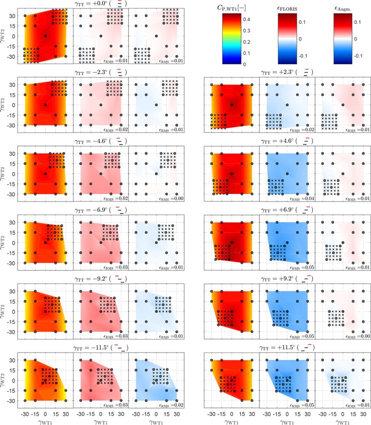
The turbine power coefficients are computed as
PWTi
CP,i = , (29)
0.5ρAV∞ (YWTi , zh , 0)3
where V∞ is the augmented inflow function given by Eq. (2),
evaluated at the respective turbine position YWTi and hub
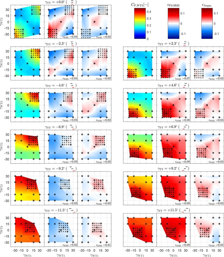
height zh . A detailed overview of the results is offered by the
figures of Appendix A, which report the power outputs and
the model errors for all wind farm configurations. For read-
ability, here a more synthetic overview of the results is pre-
sented, by condensing the information contained in Figs. A1,
A2, and A3 in the probability density plots of Fig. 10. This
figure shows the results for the baseline FLORIS model us-
ing a black dashed line, for the 11-parameter augmented
model (i.e. including only nonuniform inflow speed and sec-
ondary steering corrections) using a red solid line, and for the
27-parameter augmented model (i.e. including all additional
augmentation terms presented earlier) using a red dotted line.
Figure 10. Error distributions for each turbine for all tested con-
The root-mean-squared errors RMS are shown in the respec-
figurations, for the baseline FLORIS model (black dashed line),
tive legends. the 11-parameter augmented model (red solid line), and the 27-
Note that the FLORIS error distribution shows two peaks parameter augmented model (red dotted line).
for WT1 and WT3, indicating the presence of two uncorre-
lated errors. The 11-parameter model removes these peaks,
even though a smaller pair of peaks remains for WT2 and not insignificant – gains offered by the additional correction
WT3, indicating additional errors that only the 27-parameter terms. Finally, there is still room for improvement, possibly
augmented model is able to capture. through extra correction terms not yet explored.
Here again the trend is clear: the addition of nonuniform
speed and secondary steering substantially increases the ac-
curacy of the baseline model, with additional small – but
Wind Energ. Sci., 5, 647–673, 2020 https://doi.org/10.5194/wes-5-647-2020You can also read