Journal of Environmental Management
←
→
Page content transcription
If your browser does not render page correctly, please read the page content below
Journal of Environmental Management 277 (2021) 111430
Contents lists available at ScienceDirect
Journal of Environmental Management
journal homepage: http://www.elsevier.com/locate/jenvman
Research article
Toward building recommender systems for the circular economy: Exploring
the perils of the European Waste Catalogue
Guido van Capelleveen a, *, Chintan Amrit b, Henk Zijm a, Devrim Murat Yazan a, Asad Abdi a
a
Department of Industrial Engineering and Business Information Systems, University of Twente, the Netherlands
b
Faculty of Economics and Business Section Operations Management, University of Amsterdam, the Netherlands
A R T I C L E I N F O A B S T R A C T
Keywords: The growth in the number of industries aiming at more sustainable business processes is driving the use of the
Recommender system European Waste Catalogue (EWC). For example, the identification of industrial symbiosis opportunities, in which
Tag recommendation a user-generated item description has to be annotated with exactly one EWC tag from an a priori defined tag
European waste catalogue (EWC)
ontology. This study aims to help researchers understand the perils of the EWC when building a recommender
Industrial symbiosis
system based on natural language processing techniques. We experiment with semantic enhancement (an EWC
Circular economy
thesaurus) and the linguistic contexts of words (learned by Word2vec) for detecting term vector similarity in
addition to direct term matching algorithms, which often fail to detect an identical term in the short text
generated by users. Our in-depth analysis provides an insight into why the different recommenders were unable
to generate a correct annotation and motivates a discussion on the current design of the EWC system.
1. Introduction learning techniques (Khan et al., 2010), but the insufficient
user-generated descriptions annotated with an EWC label at an initial
One of the critical pathways to accelerate sustainable development is stage makes it impossible to train any algorithm meaningfully (Gibert
the reduction of waste emissions and primary resource use in resource- et al., 2018). To alleviate this common cold start problem, a
intensive industries. A mechanism contributing to this eco-innovation is content-based filtering approach that exploits the item description and
industrial symbiosis, which is a cooperation between industries where EWC description is more suitable. The “noise” is the primary concern,
the secondary outputs of one industry are utilized as (part of) primary omnipresent in many other tag systems, which needs to be dealt with in
inputs for the production processes of another industry (Chertow, 2000). natural language (for example, ambiguity because of misspellings,
The ontology used for annotating waste items in the European Union is synonymy, multilingualism, polysomy, hyponymy, hypernymy, idioms,
the European Waste Catalogue (EWC) (“Commission Decision on the etc.) (Golder and Huberman, 2006). To the best of our knowledge, issues
European List of Waste,” 2000). This EWC ontology supports, for related to the semantic matching of waste concepts are still poorly un
example, the identification of new symbiotic relations in eco-park derstood. Therefore, we explore the design of a method for this context
development (Genc et al., 2019) and is used in information systems to (a quite short descriptive, highly jargon-based text) that can understand
relate waste stream characterization to implications on shipping, pro the syntactic, semantic, and contextual text similarity between
cessing and disposal of waste (Pires et al., 2011). Specifically, these class user-generated item attributes and the EWC description. In our analysis,
labels, or EWC tags, typically assist users in searching for items of in we test different vector initialization methods that include context and
terest and help match users with corresponding interests. There are two semantics in short text similarity measures and compare them to a
key constraints for tagging the use of EWC codes (Gatzioura et al., 2019; baseline model that is based on a syntactic matching process. Our lin
van Capelleveen et al., 2018): (1) the tag needs to be selected from a guistic context of words is achieved through various configurations of
defined a priori tag ontology consisting of 841 EWC codes, and (2) each Word2vec model learning (Google, 2019) and the semantic alternative
item needs to be annotated with exactly one EWC code. suggestion is derived from an EWC thesaurus (U.K. Environment
The tag recommender can be framed as a classical text-classification Agency, 2006). Furthermore, we perform an in-depth analysis of rec
problem and therefore treated with supervised or unsupervised machine ommendations to find the root cause of success or failure of each
* Corresponding author.
E-mail address: g.c.vancapelleveen@utwente.nl (G. van Capelleveen).
https://doi.org/10.1016/j.jenvman.2020.111430
Received 19 March 2020; Received in revised form 4 September 2020; Accepted 25 September 2020
Available online 16 October 2020
0301-4797/© 2020 The Author(s). Published by Elsevier Ltd. This is an open access article under the CC BY-NC-ND license
(http://creativecommons.org/licenses/by-nc-nd/4.0/).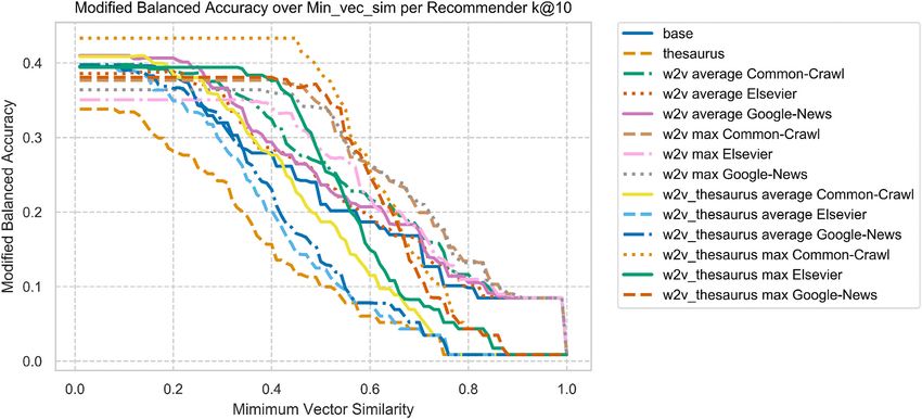
G. van Capelleveen et al. Journal of Environmental Management 277 (2021) 111430
recommender. results and social tagging systems (Mirizzi et al., 2010).
The remainder of the paper is organized as follows: Section 2 pro
vides a brief overview of tag recommendation and the previous methods 2.3. Measuring short-text semantic similarity
used to identify the context and semantics in both classical text classi
fication and short text similarity measurements. In Section 3, we explain The detection of similarity between short-text descriptions is found
the methods that we tested in our experiment. Section 4 provides the in various text-related similarity problems (e.g., conversational agents
results of the experiment, which includes a comparison of the method (Chakrabarti and Luger, 2015), linking questions with answers in Q&A
performance. Section 5 reflects on the effectiveness of the different systems (Wang and Varadharajan, 2007), plagiarism detection (Abdi
recommender models and provides an interpretation of potential causes et al., 2015), and text categorization (Ko et al., 2004)). These techniques
of recommender failure in addition to a discussion on the design of the are known as short-text semantic similarity (STSS) techniques and can
EWC ontology for tag recommendation. Finally, Section 6 summarizes be adapted to tag recommendation. STSS can be defined as a metric
our findings and presents open issues for future work. measuring the degree of similarity between pairs of small textual units,
typically with a length of less than 20 words, ignoring the grammatical
2. Background correctness of a sentence (O’Shea et al., 2008). Short contexts rarely
have common words in the exact lexical composition: hence, the key
2.1. Tag recommenders challenge of STSS is to overcome the detection of the right semantics and
context. Methods that can detect these short-text similarities are
There exists a variety of tag recommenders, each tailored to a specific string-based, corpus-based, and knowledge-based similarity measures
domain of application, enforcing different restrictions, or including ex (Gomaa and Fahmy, 2013).
tensions, which make a tag recommender unique. Many of the design Although there is no unified method that applies best to every
aspects that we are aware of in general recommender systems (van context, an appropriate method can be selected by evaluating the data in
Capelleveen et al., 2019) can also be implemented in models for tag the context of the application. Testing the effect of including each aspect
recommenders (e.g., personalization of tags (Hsu, 2013), context of a contextual or semantic relation leads to a better algorithm design for
awareness of tags (Gao et al., 2019), and video content-based tags that context. There is extensive literature on what type of aspects and
(Toderici et al., 2010)). A key aspect that makes the recommender associated methods can be dealt with, (Khan et al., 2010; Pedersen,
problem unique is its composition and governance because the tag 2008), including but not limited to boundary detection (e.g., sentence
ontology structure and “language” is shaped by the way a tag set is splitting, morphological segmentation, tokenization, topic segmenta
governed. Because of the use of a fixed taxonomy in our tag recom tion), grammar induction, lexical semantics (synonymy, multilin
mender, its problem space shows close similarity with text classification. gualism, polysomy, hyponymy, hypernymy, and idioms), text
Methods, such as string similarity class prediction (Albitar et al., 2014), representation (nouns, adjectives), word sense disambiguation
(large) scale text classification (Joulin et al., 2016; Partalas et al., 2015), (contextual meaning), text sanitation (e.g., removing stopwords,
or the most related, short text classification (Sriram et al., 2010) are the spelling corrections, and noisy data), deriving a word to a common base
basis for building an EWC tag recommender algorithm. form (stemming and lemmatization), recognition tasks (e.g., terminol
ogy extraction, named entity recognition), collocations, sentiment
2.2. Enhancing data for tag recommendation analysis, text enrichment (e.g., including a title or keywords), expanding
to second order similarity (e.g., word expansion, context augmentation,
Recently, tag recommendation has become an important subject of fuzzy matching short-text replacements), and distributional semantics
research as tags, among other textual features, have proven to be very (e.g., word embeddings).
effective in information retrieval tasks (Belém et al., 2017; Said and
Bellogin, 2014). Several scholars have studied the methods of processing 3. Methodology
natural language and modeling the data that serves as an input for
filtering algorithms with the main goal of improving the relevance of tag The design of a novel approach to identify waste concepts in short-
recommendation. Some studies indicate that incorporating item attri text waste descriptions to generate and evaluate tag recommendations
butes from different categories improves the quality of tag suggestions follow the design science research approach (Hevner et al., 2004) and
(Hölbling et al., 2010; Zhao et al., 2010). In general, data such as ab are guided by the principles of (Peffers et al., 2007). First, the problem
stract, keywords, and title (Ribeiro et al., 2015; Alepidou et al., 2011), definition is provided, followed by an explanation of the data charac
and high-level concepts derived from various modalities such as teristics. Then, we present the experimental setup and introduce our
geographical, visual, and textual information, complement each other. model.
In combination, these attributes provide a richer context that can be
used to improve tag relevance (Shah and Zimmermann, 2017). Another 3.1. Problem definition
popular principle for alleviating tag noise is topic modeling. A topic
model in a tagging context is a latent representation of a concept The problem of EWC tag recommendation is formally defined as
determined by the semantic relations between tags clustered around that follows. There is a tuple F : = (U,I,T,A), which describes the users U, the
concept (Zhong et al., 2017; Akther et al., 2012). External lexical da items I, the tags T, and the assignment of a tag by a ternary relation
tabases that contain semantic relations (i.e., WordNet, Wikipedia) sup between them, that is, A⊆U × I × T. For a user u ∈ U and a given item
port the construction of these latent topic models. These databases allow i ∈ I, the problem, to be solved by a tag recommender system, is to find a
us to create a contextual mapping between tags from a folksonomy, the tag t(u, i) ∈ T for the user to annotate the item (Godoy and Corbellini,
existing taxonomy, and the latent concepts through the translation of 2016; Belém et al., 2017). Each i ∈ I contains a short text string idesc
syntactic representation by semantic relations (Qassimi et al., 2016; (typically less than 20 words) describing a waste. This set of text strings
Zhang and Zeng, 2012; Wetzker et al., 2010; Subramaniyaswamy et al., for all items is denoted by Idesc = {idesc |i ∈ I}. The tag vocabulary T
2013). The case in (Godoy et al., 2014) shows that semantic enhance consists of tags where each t ∈ T represents a unique EWC code (at the
ment can also be used independently to increase the level of retrieval third level in the EWC ontology; see also Table 2) from the European
(recall/hit rate), supported by other works exploiting semantic data Waste Catalogue (“Commission Decision on the European List of Waste,”
bases, for example, WordNet and Wikipedia (Cantador et al., 2011; 2000). Each tag t has two components: the EWC code tewc and the EWC
Subramaniyaswamy and ChenthurPandian, 2012), DBpedia (Ben-Lha description tdesc . Another useful concept is the bag of words (BOW),
chemi and Nfaoui, 2017; Mirizzi et al., 2010), classical search engine which is a sequence of keywords extracted from a general text string.
2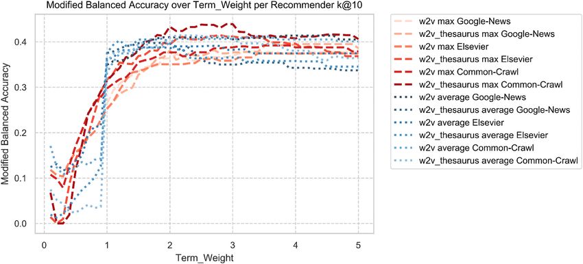
G. van Capelleveen et al. Journal of Environmental Management 277 (2021) 111430
Such a keyword representation bi for an item description using the BOW Table 2
concept is derived from idesc . Similarly, a keyword-based representation Sample illustrating the structure of the waste classification system EWC
for a tag description bt using the BOW is derived from tdesc . Finally, a (ontology) (“Commission Decision on the European List of Waste,” 2000). The
keyword-based representation of term synonyms for tag description bsyn,t full data set contains 841 classes (at level 3), each EWC description has a mean of
4.753 terms with a standard deviation of 2.038. There are 628 unique terms in
is derived from a thesaurus (described in Section 3.4). The collection of
the EWC descriptions before pre-processing, and 475 unique terms after
associated BOW pairs (each pair combining the keyword-based repre
pre-processing.
sentations of an item and a tag) is denoted as (bi ,bt ). A restriction to our
tag annotation problem is that there must be one and only one bt asso Chapter Sub Chapter Full Code Description
(Level 1) (Level 2) (Level 3)
ciated with a bi (i.e., an item is annotated by one and only one EWC tag).
In contrast to other tag recommendation problems in which the asso 03 Wastes from wood processing and the
production of panels and furniture,
ciation can be expressed on a numerical scale (such as with ratings), the
pulp, paper and cardboard
association between bt and bi is expressed as a binary value, which 03 01 Wastes from wood processing and the
means that the assigned EWC label is either correct or incorrect. production of panels and furniture
03 01 01 Waste bark and cork
3.2. Data characteristics of the “waste” domain
There are six data sources used in the experiment. The first three data Table 3
sources are characteristics of the waste domain. These are (a) data for Example of thesaurus data (U.K. Environment Agency, 2006). The full data set
prediction and evaluation, (b) the EWC tag ontology, and (c) the EWC contains 691 classes (at level 3), which means there are several EWC codes that
tag thesaurus. The other three sources are training corpora for Word2vec do not have a thesaurus description, each EWC thesaurus description has a mean
(see Section 4.1). of 8.794 terms with a standard deviation of 6.452. There are 1503 unique terms
in the EWC thesaurus description before pre-processing, and 1232 unique terms
First, we use data that consist of (1) waste descriptions specifying a
after pre-processing.
waste item for which we intend to recommend the EWC tag and (2) the
correct class label (i.e., the EWC tag) that can be used to evaluate the EWC Thesaurus entry
recommender algorithm. These data originate from industrial symbiotic 15 01 04 Cans - aluminium, Cans - metal, Metal containers - used,
workshops that were part of the EU-funded SHAREBOX project Aluminium, Aluminium cans, Aerosol containers - empty, Drums
(Sharebox Project, 2017), providing a variety of waste items with - steel, Steel drums, Aluminium foil, Containers (metal) - used,
Containers - aerosol - empty, Containers - metal (contaminated),
associated resource interests from industry. Waste items are often Contain
described using short sentences, or only a few keywords, commonly with 03 01 04 Chipboard, Sawdust, Sawdust - contaminated, Shavings - wood,
less than 10 words. These items have been annotated with an EWC tag. Timber - treated, Dust - sander, Hardboard, Wood, Wood
The EWC tag (i.e., the description at level 3 in the EWC ontology) can be cuttings
02 02 03 Food - condemned, Condemned food, Food processing waste,
seen as the class label that serves to test the prediction task of the
Animal fat, Fish - processing waste, Fish carcasses, Kitchen
recommender system. The evaluation data set is imbalanced, which waste, Meat - unfit for consumption, Poultry waste, Shellfish
means the classes are not represented equally in the test data. The processing waste, Pigs, Cows, Sheep
example data are shown in Table 1.
Next, we use the EWC ontology. This ontology is a statistical classi
fication system defined by the European Commission to be used in 3.3. Experiment setup
reporting waste statistics in the European Union in a concise manner
(“Commission Decision on the European List of Waste,” 2000). Each To test the algorithm based on an already “tagged” item set, we
EWC code represents a class that refers to a group of waste materials. attempt to assign a tag to each item using different methods and validate
The EWC code is the label of this class and is used to annotate items in the correctness of this assignment. The research setup is illustrated in
the evaluation data. An example of such an EWC structure is shown in Fig. 1. A prerequisite for all text, the short texts from each of the eval
Table 2. uation data, EWC ontology, and thesaurus data is that the natural lan
Finally, we use EWC thesaurus data in two of the suggested methods guage is pre-processed and converted into a BOW. This procedure
(see Section 3.3) to enrich the descriptions from the EWC ontology. The consists of a sequence of steps, as follows:
selected thesaurus is derived from the guidance document on the “List of
Wastes” composed by the UK Environmental Agency (see (U.K. Envi 1. All the characters are converted to lowercase and all numbers and
ronment Agency, 2006), Annex 1). An example of the thesaurus data is special characters are removed.
shown in Table 3. 2. All items are tokenized into the BOW.
3. All terms that contain less than 4 characters are removed (this
removes most non-words without much meaning, as well as
abbreviations)
4. All stop words “English” from the Natural Language Tool Kit (NLTK)
are removed (Natural Language Tool Kit, 2019). A stop word refers to
Table 1
the most frequently used word (such as “the”, “a”, “about”, and
Example of evaluation data (Sharebox) (Sharebox Project, 2017). The full test set
“also”) that are filtered before or after the NLP.
contains 311 entries describing materials, each item description has a mean of
4.945 terms per entry with a standard deviation of 3.040. There are 691 unique
5. All words are stemmed using the empirically justified Porter algo
terms in the item descriptions before pre-processing, and 479 unique terms after rithm (Porter, 1980) in NTLK (Natural Language Tool Kit, 2019).
pre-processing. The classes assigned to the entries are imbalanced over the data Stemming is the process of removing the inflectional forms and
set. sometimes the derivations of the word, by identifying the morpho
Item description EWC
logical root of a word (Manning et al., 2008).
annotation 6. All common nonsignificant stemmed terminology used in industrial
symbiosis are removed. These include “wast”, “process”, “consult”,
Iron and steel slag: Concrete tiles can be taken as one of the main 15 01 04
components “advic”, “train”, “servic”, “manag”, “management”, “recycl”,
Sawmill dust and shavings 03 01 04 “industri”, “materi”, “quantiti”, “support”, “residu”, “organ”,
Food and textile waste 02 02 03 “remaind”.
3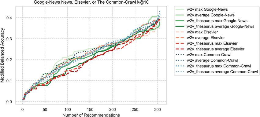
G. van Capelleveen et al. Journal of Environmental Management 277 (2021) 111430
Fig. 1. Design methodology.
7. All duplicate terms were removed from the BOW. si in a descending order.
After this set of pre-processing steps, the remainders of the BOW 3.4. Proposed methods
form the terms that are adopted in the term vector. This works as fol
lows. We first replace the now pre-processed BOW’s bi and bt by 3.4.1. Method A (base): basic term matching
numerically valued vectors vi and vt with length equal to the total In this method we simply create the binary-valued vectors vi and vt
number of unique terms appearing in either bi or bt , and set its elements from the corresponding pre-processed BOW bi and bt as discussed above
vi,j (vt,j ) equal to one if the j-th term appears in bi (bt ), and zero otherwise (see example Table 4).
(this is called the term vector initialization). Note that a basic short-text
similarity technique that relies on term vector initialization (Method A), 3.4.2. Method B (thesaurus): basic term matching, enriched with a
as in the example above, cannot detect similarity if there are no shared thesaurus (adding semantics)
terms. To mitigate this problem, we propose different term vector The second method applies in-direct term matching with the support
initialization methods (Methods B, C, and D), which use pseudo- of a semantic enhancement technique, that is, a thesaurus. The EWC
semantic similarity of the terms (described in Section 3.4). thesaurus E is exploited to increase the number of semantic links be
Before calculating the similarity score between the vectors vi and vt tween the waste item description idesc and the correct tag description
we normalize the vectors vi and vt , using feature scaling (see Zheng and tdesc . These semantically equivalent terms for the purposes of informa
Casari (2018)), that is, scaling back the magnitudes of the vectors to the tion retrieval are called synsets. The EWC thesaurus consists of a refer
range [0, 1] without changing the direction of the vector. Then, a simi ence dataset E = {(t, esyn,t )} where t is an EWC tag, and esyn,t is the
larity score is calculated to predict the classification tag bt . We selected associated synset. These synsets are derived from the ‘List of Wastes’ (U.
the classic cosine similarity measure (see Equation (1)) for measuring K. Environment Agency, 2006). For each tag t, the associated synset esyn,t
the term similarity in all four methods, as it is a robust similarity mea is also pre-processed using the steps previously described, to compose
sure (Huang, 2008). BOW bsyn,t . For each tag t, we expand the BOW bt with the BOW bsyn,t .
∑
j vi,j vt,j
si,t = CosSim(vi , vt ) = √∑ ̅̅̅̅̅̅̅̅̅̅̅
̅√∑ ̅̅̅̅̅̅̅̅̅̅̅̅ (1) Table 4
2 2
j vi,j j vt,j Example term vectors (Method A).
Equation (1) defines the similarity score si,t which is calculated by the bi bt
cosine similarity measure CosSim between two vectors vi and vt of equal food textil unsuit consumpt
length, where vi,j and vt,j denotes the elements of the term vectors vi and
vi 1 1 0 0
vt , respectively. A tag prediction task on item i results in a ranked list vt 0 0 1 1
consisting of a similarity score for each tag for that item i, denoted as
Ri = {ri,1 , ri,2 , …, ri,|T| }, where |T| is the cardinality of T, and ri,t = (t, si,t ) Item entry idesc : “Food and textile waste”. Tag entry tdesc : “materials unsuitable for
with t a specific tag and si,t the similarity score of that tag on item i. The consumption or processing” (02 02 03). Note: the terms “for, or, and” (stop words),
list is cut off for evaluation by taking the top k results from Ri by ranking and “materials, waste, processing” (non-significant terminology) are removed in
pre-processing.
4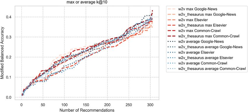
G. van Capelleveen et al. Journal of Environmental Management 277 (2021) 111430
Then, similar to the basic term matching technique (Method A), each Table 6
BOW bi is converted to a vector vi and, similarly, each BOW bt is con Examples term vectors (Method C).
verted to a vector vt (see Table 5). bi bt
powder coat paint varnish mention
3.4.3. Method C (Word2vec): using Word2vec models (adding context)
The third method is based on Word2vec. Word2vec (W2V) (Google, Direct Term Vector:
2019) is a two-layer neural net that processes text in order to produce Term vector vi 2 2 0 0 0
word embeddings, which are vector representations of a particular word Term vector vt 0 0 2 2 2
that captures the context of a word in a text. This technique can be used W2V values:
W2V weight “powder” X X .355 .379 .076
to calculate the similarity between words based on the context as an W2V weight “coat” X X .452 .491 .105
alternative or as an addition to syntactic or semantic matching tech W2V weight “paint” .355 .452 X X X
niques. In order to train how similar terms are in that context, Word2vec W2V weight “varnish” .379 .491 X X X
requires a large text corpus. Three configurations are tested, from which W2V weight “mention” .065 .058 X X X
Term Vector Config.:
the best one is selected (see Section 4.1). The purpose of testing different
Average value .266 .334 .404 .435 .091
configurations is to find a well-performing configuration that can lead to Maximum value .379 .491 .452 .491 .105
a better understanding of the use of the Word2vec approach in retrieving Weighted Term Vector:
more or alternative, albeit correct tags for EWC tag recommendation. Weighted vi using Average 2 2 .404 .435 .091
The three configurations are differentiated by the corpus used to train Weighted vt using Average .266 .334 2 2 2
Word2vec, which essentially determines which associations can be Weighted vi using Maximum 2 2 .452 .491 .105
retrieved. A heuristic set of hyper-parameter settings, each tailored to Weighted vt using Maximum .379 .491 2 2 2
that corpus, is used (and explained in Section 4.1). The three configu
Item entry idesc : “Powder coating waste”. Tag entry tdesc : “Waste paint and var
rations are as follows:
nish other than those mentioned in 08 01 11” (08 01 12). Term weight
term weight: 2. Note: the terms “and, in, other, than, those” (stop word), “waste”
• W2V Configuration “Google News”: The first configuration is based (non-significant terminology), and “08 01 11” (numbers) are removed during pre-
on the well-known pre-trained Google News Word2vec file (Google, processing.
2019).
• W2V Configuration “Common Crawl”:: The second configuration in (Croft et al., 2013). This approach replaces each zero in the direct
uses a pre-trained Word2vec file on one of the largest text corpora term vector with the average of all the Word2vec similarity values
existing today, the Common Crawl (2019), which is offered by the between the term of that dimension and each of the initially non-zero
fastText library of Facebook (Facebook Inc., 2019). terms of the other vector.
• W2V Configuration “Elsevier”: The third configuration is based on • Term vector configuration: “Maximum W2V Similarity”: The
a “waste” data corpus manually constructed by scraping the “ab “Maximum W2V Similarity” is an adaptation of the similarity measure
stract” and the “introduction” section from the available academic in (Crockett et al., 2006). This approach replaces each zero in the
papers indexed by Elsevier Scopus (Elsevier, 2019) retrieved through direct term vector with the maximum Word2vec similarity value
the search query “waste”. Then, the Word2vec model is trained using between the term of that dimension and each of the initially nonzero
the Word2vec implementation in the Gensim library (Řehůřek, terms of the other vector.
2019).
In case Word2vec fails to provide a similarity score for some terms,
After training the model, we can assign Word2vec similarities to the we use the score of Ratcliff/Obershelp pattern recognition (Ratcliff and
dimensions of the term vector. To do that, we first create a direct term Metzener, 1988). Ratcliff/Obershelp computes the similarity between
vector using the vector creation procedure as described above, where two terms based on the number of matching characters divided by the
each non-zero element is multiplied with a so-called term weight value to total number of characters in the two terms.
determine the balance between the direct term matching and the
context-based Word2vec similarity scores. The latter scores are calcu 3.4.4. Method D (Word2vec thesaurus): using Word2vec models (adding
lated by Word2vec to indicate the degree of similarity between two context), enriched with a thesaurus (adding semantics)
terms that appear in bi and bt , respectively. Two approaches are tested to Method D is a combination of Method B and Method C. It employs the
represent the context-based term similarity created by the Word2vec thesaurus as used in the Method B, thereby, enriching the dataset with a
similarity score(s), which are named the “Average W2V Similarity” and larger variety of terms. After obtaining the term vectors vi and vt using
the “Maximum W2V Similarity”. Both methods are illustrated with an method B, we apply Method C to include the Word2vec values in the
example in Table 6. term vector which together create the weighed vectors vi and vt .
• Term vector configuration: ‘Average W2V Similarity’: The
“Average W2V Similarity” is an adaptation of the similarity measure
Table 5
Example term vectors (Method B).
bi bt
food textil unsuit consumpt condemn anim fish carcass kitchen meat unfit poultri shellfish pig cow sheep
vi 1 1 0 0 0 0 0 0 0 0 0 0 0 0 0 0
vt 1 0 1 1 1 1 1 1 1 1 1 1 1 1 1 1
Item entry idesc : “Food and textile waste”. Tag entry tdesc : “materials unsuitable for consumption or processing” (02 02 03). Thesaurus entry eewc : “Food - condemned,
Condemned food, Food processing waste, Animal fat, Fish - processing waste, Fish carcasses, Kitchen waste, Meat - unfit for consumption, Poultry waste, Shellfish processing
waste, Pigs, Cows, Sheep” Note: the terms “for, or, and” (stop words), “materials, waste, processing” (non-significant terminology), and “fat” (less than 4 characters before
stemming) are removed during pre-processing.
5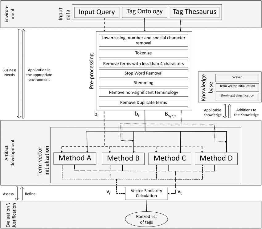
G. van Capelleveen et al. Journal of Environmental Management 277 (2021) 111430
4. Algorithm performance test a smaller window size captures more dependency-based embeddings (e.
g., the words that are most similar, synonyms or direct replacements of
To assess the performance of the proposed set of methods and to the originated term).
provide comparative measures, an experiment was conducted. First, the
configuration settings for training the Word2vec models are explained. 4.2. Evaluation metrics
This is followed by a set of definitions of the evaluation metrics and the
optimization process for the parameters of the tag recommender. A series of commonly applied evaluation metrics are used to evaluate
Finally, the methods are compared given their optimal parameter and compare the performance of our proposed methods for tag recom
configurations. mendation (Said and Bellogín, 2018; Ekstrand et al., 2011). All the ex
periments were conducted in an off-line setting. Our EWC tag problem is
a multi-class classification problem in which the EWC code acts as the
4.1. Word2vec model and hyperparameters class label. A multi-class classification problem is a classification task
with more than two classes under the assumption that each item is
Three different configurations (see Table 7) were tested to find a assigned one and only one class label. Multi-class data, such as ours, are
strong Word2vec model to represent our proposed context-based ap often imbalanced, which means that the classes are not represented
proaches (Methods C and D). equally. Therefore, the evaluation uses metrics at both the micro and
The first configuration is based on the “Google News” data set which macro levels (Scikit-learn developers, 2020). We measured the preci
is a well-known baseline for Word2vec experiments, but not optimized sion, recall, accuracy, F-measure (or F1), mean reciprocal rank (MRR),
for jargon. To align with the semantic use of rare terms and jargon, we and discounted cumulative gain (DCG). We measure precision, recall,
created two other configurations: that is, the “Common Crawl” and the accuracy, and F1 at the micro-level because micro-averaging treats all
“Elsevier” configuration. The “Common Crawl” configuration is based classes by their relative size, which better reflects imbalanced data
on one of the largest data sets on which Word2vec has been globally subsets. Furthermore, we measure the balanced accuracy at the macro
trained, and it uses the latest continuous bag of word techniques level. The Greek letters μ, M, and γ indicate micro-, macro-, and
implemented by Facebook. The pre-trained Word2vec model uses fast balanced-averaging, respectively. The other metrics MRR and DCG are
Text which exploits enriched word vectors with subword information to rank-based metrics. Rank-based metrics measure a ranked list using a
optimize the performance of rare words. This is because fastText can function that discounts a correct tag when found at a lower position in
compute word representations for words that did not appear in the the list.
training data (Bojanowski et al., 2017). The “Elsevier” configuration was First, we create a matrix P with a prediction si,t , obtained from the
created from scratch. The key is to construct a more jargon containing similarity measure CosSim() in Equation (1), between each item i and
data set to train Word2vec. We collected data from Elsevier Scopus each EWC tag t. From P, we can obtain the ranked list of predictions Ri
through a search of abstracts and introductions of academic papers that (see Section 3.3). The precision, recall, accuracy, and F-measure are
are related to the search query “waste”. Of the more than 8e+5 indexed metrics measured at the list level. A metric at the list level measures a list
documents, we were able to retrieve 3.57e+5 documents, for which the at a particular k, meaning that if the correct tag is among the first k
raw text content was downloaded through the Scopus API. We removed ranked tags, it is considered as a correct list of tags and thus a correct
the numbers, links, citations, and page formatting hyphenations so that recommendation (Baeza-Yates and Ribeiro-Neto, 2011). The relevance
only the clean sentences remain. We trained the Word2vec using this of tag prediction is evaluated in a binary fashion; that is, a list of tag
data and the configuration settings as noted in Table 7. Because the predictions can only be classified as correct or incorrect recommenda
Elsevier dataset is targeted to maximize the retrieval of jargon used in tion. This means that, for every i, the recommendation is a list of the k
the waste domain, we configured the parameters to support this highest predictions (si,t1 , si,t2 , …, si,tk ) in Ri , where k is the maximum
accordingly. The number of dimensions of learning word embeddings is number of ranked tags. First, we define the class-level metrics, and then
set to 1000 (where the rule of thumb is 50–300 for a good balance in we show how the list-level metrics at the micro and macro levels are
performance), and the minimal term count is lowered to 1, which should defined, and finally, we present the rank-based metrics.
favor learning word embeddings for rare terms (Patel and Bhattachar
yya, 2017; Mikolov et al., 2013). We use the heuristic of 10 (pos/neg) for 4.2.1. Tag- or class-level metrics
the window size (based on (Pennington et al., 2014)). The window size The set of tags T (i.e., level 3 EWC descriptions) represents the classes
determines how many words before and after a given word are included for evaluating our multi-class tag assignment problem. In the evaluation
in the context that Word2vec uses to learn relationships. A larger win of a binary classification, tp denotes the number of true positives, fp is
dow size typically tends to capture more domain context terms whereas the number of false positives, tn is the number of true negatives, and fn is
the number of false negatives. In multi-class evaluation, we use a class-
Table 7 based definition of true positives tp, false positives fp, false negatives fn,
Description of the data, and the Word2vec model hyperparameter settings. and true negatives tn. We use t to indicate that the counts of tp,fp, fn, and
Google ( Common Crawl ( Elsevier ( tn are measured for a specific class (i.e., tag). A true positive tpt for a tag t
Google, 2019) Grave et al., 2018) Elsevier, 2019) is when the correct tag label is class t and the list of predicted tag labels
No. terms/pag. 100E9 words 1.5E11 pages 3.57E5 docs contains the correct tag label. A false positive fpt for a tag t is when the
File Size NA 234 TiB 2.41 GB correct tag label is not class t and a list of predicted tags contains the
Training Platform: correct tag label. A false negative fnt for a tag t is when the correct tag
Framework Word2vec Word2vec Word2vec
label is class t, and the list of predicted tag labels does not contain the
(Google) (fastText) (Gensim)
Model configuration: correct tag label. A true negative tnt for a tag t is when the correct tag
Architecture Continuous CBOW Continuous label is not class t, and a list of predicted tags does not contain the correct
Skip-gram Skip-gram tag label.
File size 3.6 GB 7.1 GB 4.9 GB
The precision related to tag t (Equation (2)) is the number of
Word embedding 300 300 1000
(Dimension size)
correctly recommended tags t divided by all instances in which tag t has
Epochs NA 5 5 been recommended.
Minimal term count 5 NA 1
tpt
Window size 5pos/15 neg 5 pos/10 neg 10pos/10neg Precisiont = (2)
N-gram – 5 – tpt + fpt
6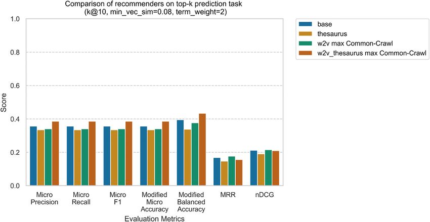
G. van Capelleveen et al. Journal of Environmental Management 277 (2021) 111430
The recall related to tag t (Equation (3)) is the number of instances classes T, we typically measure a balanced score instead. Equation (12)
that are correctly tagged with t divided by the total number of instances denotes balanced accuracy (Scikit-learn developers, 2020), as used for
for which tag t would be the correct label. multi-class classification which avoids inflated performance estimates
tpt on imbalanced datasets. Balanced accuracy is the macro-average of the
Recallt = (3) recall scores.
tpt + fnt
1 ∑
The F-measure (or F1 score) (Equation (4)) is a different measure of a BalancedAccuracyγ = Recallt = RecallM (12)
test’s accuracy that evaluates the precision and recall in a harmonic |T| t∈T
mean. However, in the implementation of sklearn (Scikit-learn developers,
Precisiont ⋅Recallt 2020), the balanced accuracy (see Equation (13)) does not count the
F − measuret = 2⋅ (4) scores for classes that did not receive predictions. Let X denote the set of
Precisiont + Recallt
all tags that have been predicted at least once, with |X| the cardinality of
Accuracy (Equation (5)) is the fraction of measurements of correctly X. Then we have:
identified tags as either truly positive or truly negative out of the total
number of items. 1 ∑
ModifiedBalancedAccuracyγ = Recallt (13)
|X| t∈X
tpt + tnt
Accuracyt = (5)
tpt + tnt + fpt + fnt
4.2.4. Rank-based Metrics
4.2.2. Micro-level metrics Finally, we define rank-based evaluation metrics. The MRR (see
When we evaluate the classes at a micro level, we count all tpt , tnt , fpt Equation (14)) is a rank measure appropriate for evaluating a rank in
and tnt globally, that is, summing the values in the numerator and de which there is only one relevant result, as it only uses the single highest-
nominator prior to division. Equation (6) denotes the micro precision as ranked relevant item (Baeza-Yates and Ribeiro-Neto, 2011). This metric
used for multi-class classification, that is, a generalization of the preci is similar to the average reciprocal hit-rank (ARHR), defined in (Desh
sion for multiple classes t. pande and Karypis, 2004). Let R be the set of all recommended lists, and
∑ let Z denote the set of all items for which the recommended list of tags
t∈T tpt contains at least one correct tag in the top k tags. Define ranki as the
Precisionμ = ∑ (6)
t∈T (tpt + fpt ) position of the correct tag in Z. Then, the MRR is defined as
Equation (7) denotes the micro-recall, as used for multi-class clas 1 ∑ 1
MRR = (14)
sification, that is, a generalization of the recall for multiple classes t. |R| i∈Z ranki
∑
Recallμ = ∑ t∈T tpt
(7) Another useful evaluation metric is the DCG (Järvelin and
t∈T (tpt + fnt ) Kekäläinen, 2002). In recommender systems, relevance levels can be
Equation (8) denotes the micro F-measure (or micro F1 score) as used binary (indicating whether a tag is relevant or irrelevant for an item) or
for multi-class classification, that is, a generalization of the F-measure graded on a scale (indicating a tag has a varying degree of relevance
for multiple classes t. with an item, e.g., 4 out of 5). In our evaluation, the relevance score on
an item is a binary graded relevance score of a tag (i.e., a tag is either
F − measureμ = 2⋅
Precisionμ ⋅Recallμ
(8) correct or incorrect). The DCGi (Equation (15)) is a cumulation of all
Precisionμ + Recallμ binary graded relevance scores from position 1 to k in the ranked list of
tags for an item i, with reli,p the binary graded relevance score at position
Equation (9) denotes the micro accuracy as used for multi-class
p, which is discounted by a log function in the denominator that pro
classification, that is, a generalization of the accuracy, defined over all
gressively reduces the impact of a correctly ranked tag when found at a
tags. The micro accuracy is the fraction of correct predictions over the
lower ranked position.
total number of predictions (regardless of the positive or negative label).
∑ ∑k
2reli,p − 1
Accuracyμ = ∑ t∈T (tpt + tnt )
(9) DCGi = (15)
(tpt + tnt + fpt + fnt ) p=1
log2 (p + 1)
t∈T
As the tnt inflates the accuracy when there are many classes T, we In our case each recommended list contains at most one correct tag,
typically measure (see (Scikit-learn developers, 2020)) the test result which reduces to the following (see Equation (16)):
from the perspective of the correct class t for a multi-class evaluation. ⎧
Therefore, the modified micro accuracy is the fraction of correct pre ⎪
⎨ 0, if the recommended list contains no correct tag
dictions for a class t over the number of predictions for items for which DCGi =
⎪
1
, if the correct tag is found at position p
⎩
the correct tag label is t, as denoted in Equation (10), which is similar to log2 (p + 1)
micro recall. (16)
∑
t∈T tpt The DCG (Equation (17)) is the mean of the DCGi of all recommended
ModifiedAccuracyμ = ∑ = Recallμ (10)
t∈T (tpt + fnt )
lists in R.
1 ∑
4.2.3. Macro-level metrics nDCG = DCGi (17)
|R| i∈Z
When we evaluate all classes at a macro level, we calculate the
metrics for each class t, and then calculate the (unweighted or weighted) While in many recommender evaluations it is common to provide a
mean. Equation (11) denotes the unweighted macro accuracy (Sokolova normalized discounted cumulative gain (nDCG), this does not apply to
and Lapalme, 2009). binary graded multi-class evaluation. This is because the DCGi would be
normalized over the same ideal ranking. Let the ideal discounted cu
1 ∑ tpt + tnt
AccuracyM = (11) mulative gain IDCGi (Equation (18)) represent the maximum possible
|T| t∈T tpt + fnt + fpt + tnt
DCGi . This IDCGi is calculated as DCGi for the sorted list with a
In practice, as the tnt inflates the accuracy when there are many maximum length of positions k of all relevant tags ordered by their
7
G. van Capelleveen et al. Journal of Environmental Management 277 (2021) 111430
binary graded relevance score, with k as the number of predicted tags term similarity based on the Word2vec similarity score(s). Fig. 2 ex
and reli,p as the binary graded relevance score of the tag at position p. plains the initialization of the term weight parameters. After some noise
at 0–0.5, most of the recommenders show an increasing modified
∑k
IDCGi =
2reli,p − 1
=1 (18) balanced accuracy with a decreasing slope between 0.5 and 2.0 followed
p=1
log2 (p + 1) by a slight decrease (2.0–5.0), resulting in a concave function with a
maximum around term-weight equal to 2. Therefore, we selected 2 as
The nDCGi (see Equation (19)) for a single ranked list of tags for item
the term weight parameter value for our experiment, as this seems to
i is denoted as the fraction of DCGi over the IDCGi .
provide close to the best results for all recommenders.
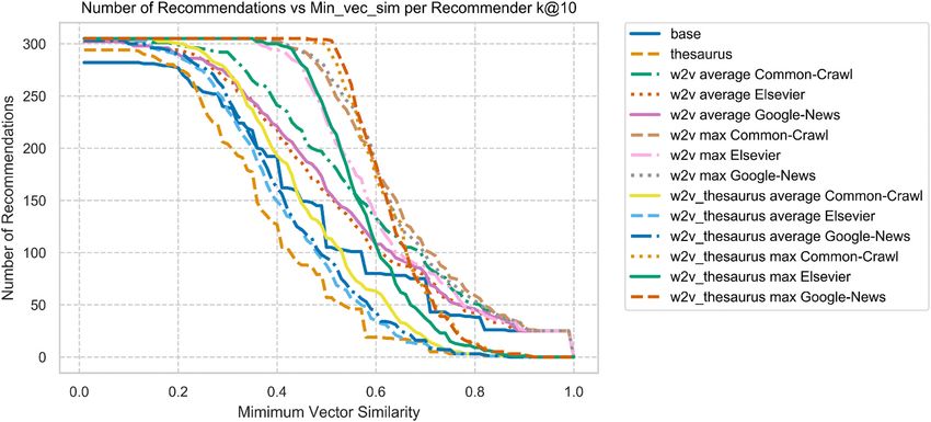
DCGi DCGi We also perform a sensitivity analysis with respect to the minimum
nDCGi = = = DCGi (19)
IDCGi 1 vector similarity min vec sim. Two important aspects should be consid
ered here. First, it concerns a multi-class recommender problem with
Because the gain is only achieved at the correct tag, which is the first
many tags (each tag forms a class). In addition, a term match between
position in a ranked list of tags, normalization is irrelevant as the IDCG is
two short-text descriptions cannot always be established (see Fig. 4; the
then equal to 1. Therefore, we adopted the DCG instead of nDCG in our
number of list recommendations generated is lower than 311, which is
experiment.
the number of items for which recommendation is required). Hence,
when the vector similarity is increased to favor better recommendations,
4.3. Parameter setting of the recommenders it may, unfortunately, also cut off the number of correct recommenda
tions. As can be observed in Fig. 3 the modified balanced accuracy drops
A few selection criteria are applied as a prerequisite for our com almost immediately, (as opposed to recommender systems in which a
parison in Section 4.4. First we need to find the optimal initialization for multi-fold of recommendations can be correct). This explains the
two parameters. Parameter (1) determines the term weight assigned to initialization of the minimum vector similarity parameter to a value of
the position in a term vector for which a term is present in the BOW. This 0.08 (just before the decreasing slope of the first recommender).
can increase or decrease the importance of Word2vec similarity values
that are assigned to positions in the vector for which the term is not 4.3.2. Configuration selection
present in the BOW. This balances the effect of exact term matches in To support the selection of the Word2vec data configuration Fig. 5
relation to Word2vec similarity scores. Parameter (2) determines the shows the result of a sensitivity analysis between the number of rec
minimum vector similarity (which we refer to as min vec sim). Next, we ommendations caused by adjusting the min vec sim parameter (2) (see
need to select the optimal W2V configuration upon which Word2vec is Fig. 4), and the effect on the modified balanced accuracy. This analysis
trained to calculate similarities for our “waste” domain, that is, highlights the three Word2vec configurations with different line styles
comparing, the “Google News” configuration, the “Common Crawl” and colors. The preferred setting for our recommender would be to
configuration, and the “Elsevier” configuration. Finally, we need to provide a recommendation in as many scenarios as possible while sus
select the better of the two approaches proposed to represent the taining a satisfactory modified balanced accuracy. Consistent with the
context-based term similarity created by the Word2vec similarity score previous modified balanced accuracy results, it seems that the best
resulting in the term vector configuration: “Average W2V Similarity” or representations of phrases are learned by a model with the “Common
“Maximum W2V Similarity”. Crawl” configuration (dotted lines), reflected by the higher accuracy
results over the curve by all recommenders using this configuration.
4.3.1. Parameter setting The term vector configuration “Maximum W2V Similarity” is selected
To determine the optimal term weight, we test the sensitivity of for two reasons. First, the lower sensitivity of the configuration provides
term weight for all recommenders using method C or D to detect where a more reliable modified balanced accuracy (see Fig. 2). Second, in Fig. 6
the best modified balanced accuracy is achieved. The term weight de the sensitivity analysis between the number of recommendations as a
termines whether the CosSim-based match (see Section 3) puts more result of adjusting Parameter (2), the min vec sim, and the modified
emphasis on a term that exists in both the BOW bi and bt or on a term that balanced accuracy shows that the “Maximum W2V Similarity”
exists only in one BOW; thus, a match is created using a representation of
Fig. 2. Influence of parameter (1) term weight on the modified balanced accuracy. Spearman’s Rank values range from ρ = − 0.04 to 0.98 indicating that for some
algorithms, there seems to be an positive underlying fitting monotonic relationship between the parameter variables (ρ > 0.9), but most algorithms are affected by
the noise in [0–1] or the downwards slope in [2.0–5.0].
8
G. van Capelleveen et al. Journal of Environmental Management 277 (2021) 111430
Fig. 3. Influence of parameter (2) “Minimum Vector similarity” on the modified balanced accuracy achieved by a recommender. Spearman’s Rank values range from
ρ = − 0.94 to − 0.99 indicating that for all algorithms, there seems to be an underlying fitting negative monotonic relationship between the parameter variables
(ρ > 0.9).
Fig. 4. Influence of parameter (2) “Minimum Vector similarity” on the number of recommendations generated by the recommender. Spearman’s Rank values range
from ρ = − 0.95 to − 0.99 indicating that for all algorithms, there seems to be an underlying fitting negative monotonic relationship between the parameter variables
(ρ > 0.9).
configuration (dashed lines) mostly outperforms the modified balanced metrics. The micro and macro evaluation metrics (e.g., micro preci
accuracy of the “Average W2V Similarity” configuration (dotted lines). sion, modified balanced accuracy) measure at a list level, implying that
if the correct tag is among the first k ranked tags, it is considered as a
correct list of tags and thus a correct recommendation. These list-level
4.4. Comparison of methods metrics show a noticeable decrease in performance for recommender
methods B and C, while the recommender method D shows an increase
To compare the methods we use the optimal configuration as (all in comparison with method A). The micro results, that is, the micro
explained in Section 4.3. These are (A) base-line method, (B) thesaurus, precision, micro recall, micro accuracy, and micro F1 scores are all
(C) Word2vec in the configuration “Common Crawl” using the context- equal, as can be observed in Table 8. This can be explained as follows.
based term similarity “Maximum W2V Similarity”, and (D) Word2vec + First, a fpfor tag t is also a fn for (correct) t , as denoted in Equation (20)
′
thesaurus in the configuration “Common Crawl” using the context-based
where t ∕ = t.
′
term similarity “Maximum W2V Similarity”. The prediction task was
evaluated with k = 10 using a min vec sim of 0.08 and a term weight of 2. fpt = fnt′ (20)
Fig. 7 shows the performance of these four methods reporting the scores
Similarly, a fn for tag t is also a fp for tag t (i.e., the tag that is pre
′
for each of the evaluation metrics defined in Section 4.2. The detailed
sumed to be the correct tag).
data underlying Fig. 7 are presented in Table 8.
As it concerns an evaluation of recommender systems on a multi- fnt = fpt′ (21)
class classification problem, we measured a recommendation (a list of
From this, it follows that the sum of all fpt is equal to the sum of all fnt
tags) at the micro level, at the macro level and by using rank-based
9G. van Capelleveen et al. Journal of Environmental Management 277 (2021) 111430
Fig. 5. Influence of different Word2vec configurations for learning word embeddings that affect the modified balanced accuracy of the recommenders. Spearman’s
Rank values range from ρ = 0.97 to 0.99 indicating that for all algorithms, there seems to be an underlying fitting positive monotonic relationship between the
parameter variables (ρ > 0.9).
Fig. 6. Influence of term vector configuration “Average” or “Max” on the modified balanced accuracy of recommenders. This is a pivot of Fig. 5, hence identical
ρ values.
(see Equation (22)), which gives identical results for precisionμ , recallμ , 2.2e-16 for all data. Therefore, to statistically compare the performance
F − measureμ , and accuracyμ . we use two non-parametric statistical significance tests (see Table 9). For
∑ ∑ the list-based metrics, we use McNemar’s test (McNemar, 1947), which
fpt = fnt (22) is a non-parametric test for paired nominal data. For the rank-based
metrics, we use the Wilcoxon’s signed rank test (Wilcoxon and Wilcox,
t∈T t∈T
On the other hand, the rank-based evaluation DCG, which assigns a 1964), which is a non-parametric test for paired ordinal and continuous
score based on the position where a correct tag is found in the list, shows data.
a decreasing rank for Method B, whereas the rank of Method C and D are The Wilcoxon test compares the alternative versions of the proposed
almost similar to that of A. The MRR in our context assigns a higher score algorithms (B,C,D) to the baseline algorithm (A) based on the paired
to a lower-ranked correct tag than DCG, as reflected in the MRR results results (i.e., between binary evaluation values of recommendations)
that show a greater difference. Although an increase in micro precision without making distributional assumptions on the differences (Shani
for method D benefits the support that can be provided during the EWC and Gunawardana, 2011). Such a hypothesis is non-directional, and
classification task in online waste exchange platforms, the results are therefore the two-sided test is applied. We tested by using an α of 0.05,
only marginal. Concerning the number of recommendations provided, implying a 95% confidence interval. The resulting Wilcoxon Critical T
we notice an increase (282–305) for methods using the thesaurus and values for each sample size n (reported in Table 9) were obtained from
Word2vec. the qsignrank function in R (Dutang and Kiener, 2019). The Wilcoxon
To understand the significance of the results, we apply a significance test is configured to adjust for the ranking in the case of ties. Further
test. Our data are non-normally distributed, indicated by the Shapiro- more, it is initialized with the setting that accounts for the likely bino
Wilk (Shapiro and Wilk, 1965) test results that report p-values of < mial distribution in a small data set by applying continuity correction.
10G. van Capelleveen et al. Journal of Environmental Management 277 (2021) 111430
Fig. 7. Evaluation metrics.
Table 8
Comparison of recommenders on top-k tag prediction task. Method C and D use configuration “Common Crawl”, and method “Maximum Vector Similarity”, term_
weight = 2, min_vec_sim = 0.08, evaluation k@10.
Method #Recommended Items Micro Precision Micro Recall Micro F1 Modified Micro Modified Balanced MRR DCG
(list) (list) (list) (list) Accuracy (list) Accuracy (list) (rank) (rank)
A: baseline 282 0.3569 0.3569 0.3569 0.3569 0.3952 0.1683 0.2120
B: thesaurus 294 0.3344 0.3344 0.3344 0.3344 0.3378 0.1473 0.1906
C: Word2vec 305 0.3408 0.3408 0.3408 0.3408 0.3765 0.1769 0.2155
[l]D: Word2vec + 305 0.3859 0.3859 0.3859 0.3859 0.4332 0.1563 0.2100
thesaurus
Table 9
Statistical significance of recommender comparison: McNemar test and Wilcoxon signed rank test.
Test Compared Method Metric Type n X2 Critical T T α p
McNemar two-sided A-B List 60 1.067 – – 0.05 0.3017
McNemar two-sided A-C List 21 1.191 – – 0.05 0.2752
McNemar two-sided A-D List 21 1.191 – – 0.05 0.2752
Wilcoxon two-sided A-B Rank 117 – 2732 2724.5 0.05 0.0476
Wilcoxon two-sided A-C Rank 72 – 965 1093 0.05 0.2089
Wilcoxon two-sided A-D Rank 131 – 3471 4519 0.05 0.6518
As is evident from Table 9, only the test comparing Method A-B has a 5. Discussion
T lower than the Critical T; hence, the difference between Method A and
Method B is significant at p ≤ 0.05 (also reflected in the p-value of the 5.1. Causes for incorrect EWC tag recommendations
test A-B, which is 0.0476 this value is less than the significance level α =
0.05). We can conclude that the median weight of Method B is signifi To identify the causes behind the relatively low performance of the
cantly different from the median weight of Method A. However, both the tag recommenders, we analyze how each of the ranked lists of EWC tags
McNemar Test and the Wilcoxon rank test comparing Method A-C and for a waste item is generated. The analysis considers all recommenda
Method A-D report p-values lower than the significance level α = 0.05. tions produced by the four compared recommenders (see Section 4.4),
However, for methods C and D n < 30 which indicates that there is only for all the 311 waste items. Table 10 provides a list of causes found,
marginal performance change. McNemar’s test (McNemar, 1947) is ranked by the frequency of observation, which explains why a filtering
typically valid when the number of discordant pairs exceeds 30 algorithm failed to retrieve the correct EWC tag. For an identical item,
(Rotondi, 2019). Therefore, we cannot confirm or disprove the statistical several causes may be registered for every recommendation generated
validity of the list-based metrics for C and D. To investigate whether all by a different method. However, only one unique cause is counted for
the results are significant, a larger data set is required. A positive remark each item for which all recommenders attempt to suggest a tag.
on the significance of the results is that combining a thesaurus with the Suggestions are provided in three areas to increase the performance
contextualized Word2vec approach does not significantly worsen the of NLP-based EWC tag recommendation. First, the analysis of natural
ranking, but does increase the number of items that can be recom language may be improved by adding descriptions from the higher levels
mended. This is a positive characteristic that is helpful in content-based in the EWC hierarchy. These contain the originating industry specifics,
algorithms, which are built with the aim of bootstrap recommendation. which may help to distinguish between many similar types of EWC code
11You can also read