Drivers and modelling of blue carbon stock variability in sediments of southeastern Australia
←
→
Page content transcription
If your browser does not render page correctly, please read the page content below
Biogeosciences, 17, 2041–2059, 2020
https://doi.org/10.5194/bg-17-2041-2020
© Author(s) 2020. This work is distributed under
the Creative Commons Attribution 4.0 License.

Drivers and modelling of blue carbon stock variability
in sediments of southeastern Australia
Carolyn J. Ewers Lewis1,5 , Mary A. Young2 , Daniel Ierodiaconou2 , Jeffrey A. Baldock3 , Bruce Hawke3 ,
Jonathan Sanderman4 , Paul E. Carnell1 , and Peter I. Macreadie1
1 School of Life and Environmental Sciences, Centre for Integrative Ecology, Deakin University,
221 Burwood Highway, Burwood, Victoria 3125, Australia
2 School of Life and Environmental Sciences, Centre for Integrative Ecology, Deakin University,

Princes Highway, Warrnambool, Victoria 3280, Australia
3 Commonwealth Scientific and Industrial Organisation, Agriculture and Food, PMB 2,

Glen Osmond, South Australia 5064, Australia
4 Woods Hole Research Center, 149 Woods Hole Road, Falmouth, MA 02540, USA
5 Department of Environmental Sciences, University of Virginia, 291 McCormick Road, Charlottesville, VA 22903, USA

Correspondence: Carolyn J. Ewers Lewis (ce8dp@virginia.edu)

Received: 26 July 2019 – Discussion started: 9 August 2019
Revised: 14 January 2020 – Accepted: 10 February 2020 – Published: 16 April 2020

Abstract. Tidal marshes, mangrove forests, and seagrass          thropogenic variables were of least importance. Our model
meadows are important global carbon (C) sinks, commonly          explained 46 % of the variability in 30 cm deep sediment C
referred to as coastal “blue carbon”. However, these ecosys-     stocks, and we estimated over 2.31 million Mg C stored in the
tems are rapidly declining with little understanding of what     top 30 cm of sediments in coastal blue C ecosystems in Vic-
drives the magnitude and variability of C associated with        toria, 88 % of which was contained within four major coastal
them, making strategic and effective management of blue          areas due to the extent of blue C ecosystems ( ∼ 87 % of to-
C stocks challenging. In this study, our aims were three-        tal blue C ecosystem area). Regionally, these data can inform
fold: (1) identify ecological, geomorphological, and anthro-     conservation management, paired with assessment of other
pogenic variables associated with 30 cm deep sediment C          ecosystem services, by enabling identification of hotspots for
stock variability in blue C ecosystems in southeastern Aus-      protection and key locations for restoration efforts. We rec-
tralia, (2) create a predictive model of 30 cm deep sediment     ommend these methods be tested for applicability to other
blue C stocks in southeastern Australia, and (3) map regional    regions of the globe for identifying drivers of sediment C
30 cm deep sediment blue C stock magnitude and variabil-         stock variability and producing predictive C stock models at
ity. We had the unique opportunity to use a high-spatial-        scales relevant for resource management.
density C stock dataset of sediments to 30 cm deep from
96 blue C ecosystems across the state of Victoria, Australia,
integrated with spatially explicit environmental data to reach
these aims. We used an information theoretic approach to         1   Introduction
create, average, validate, and select the best averaged gen-
eral linear mixed effects model for predicting C stocks across   Vegetated coastal wetlands – particularly tidal marshes, man-
the state. Ecological drivers (i.e. ecosystem type or ecolog-    grove forests, and seagrass meadows – serve as valuable or-
ical vegetation class) best explained variability in C stocks,   ganic carbon (C) sinks, earning them the term “blue carbon”
relative to geomorphological and anthropogenic drivers. Of       (Nellemann et al., 2009). Still, an increasing proportion of
the geomorphological variables, distance to coast, distance to   these ecosystems are being degraded and converted, and with
freshwater, and slope best explained C stock variability. An-    pressures associated with human population growth the com-
                                                                 petition for land use in coastal zones continues to increase.

Published by Copernicus Publications on behalf of the European Geosciences Union.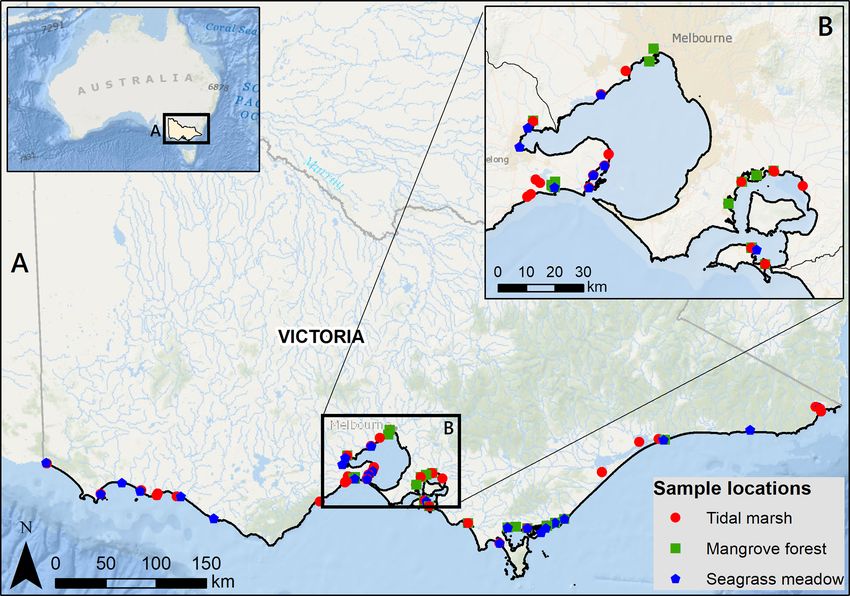
2042                                         C. J. Ewers Lewis et al.: Drivers and modelling of blue carbon stock variability

With the current momentum for including blue C ecosys-                 Considerable variability in sediment C stocks has also
tems in global greenhouse gas inventories, there is a need          been observed across species of vegetation. Lavery et
to quantify the magnitude of C stocks and fluxes, especially        al. (2013) compared 17 Australian seagrass habitats encom-
in the sediments where the majority of the long-term C pool         passing 10 species and found an 18-fold difference in sedi-
persists (Mcleod et al., 2011). However, global and regional        ment C stocks across them. Similarly, saltmarsh species dif-
assessments of blue C reveal large variability in sediment C        fer not only in magnitude of C stocks but also in their capac-
stocks, both on small and large scales (Ewers Lewis et al.,         ity to retain allochthonous C (Sousa et al., 2010a). Species
2018; Liu et al., 2017; Macreadie et al., 2017a; Ricart et al.,     richness within an ecosystem type may also play a role in
2015; Sanderman et al., 2018). Identification of environmen-        sediment C stock variability. In a global assessment, man-
tal variables driving differences in sediment C stocks in blue      grove stands with five genera had 70 %–90 % higher sedi-
C ecosystems has become a key objective in blue C science           ment C stocks per unit area compared to other richness levels
and a necessary next step for quantifying C storage as an           (one to seven species stands; Atwood et al., 2017).
ecosystem service. Knowledge of such drivers is also impor-            Beyond vegetation type, geomorphological factors appear
tant for coastal blue C management, including identification        to be most important when considering fine spatial scale sed-
of hotspots to prioritize for conservation, as well as maxi-        iment C stock variability (Sanderman et al., 2018). Elevation
mization of C gains through strategic restoration efforts.          is likely an important driver of C stock variability in blue C
   Drivers of sediment C stock variability are innately dif-        ecosystems. Generally, the majority of the variability in C
ficult to identify in that the stocks represent the net result of   sequestration rates is linked to differences in sediment sup-
many complex processes acting simultaneously, simplified as         ply and inundation (Chmura et al., 2003). At lower eleva-
follows: (1) production of autochthonous C, (2) trapping and        tions, faster sediment deposition may aid in C sequestration
burial of autochthonous and allochthonous C, and (3) rem-           by trapping organic matter from macrophytes and microbes
ineralization and preservation of buried and surface C. Spa-        growing on soil surfaces (Connor et al., 2001). At higher ele-
tial variability in sediment blue C stocks resulting from these     vations, tidal flooding is less frequent, providing less oppor-
processes exists in hierarchical levels across global, regional,    tunity for particles and C to settle out of the water column,
local, and ecosystem patch level scales (Ewers Lewis et al.,        resulting in a lower contribution of allochthonous C from
2018; Sanderman et al., 2018) and may be influenced by cli-         marine or other sources compared to lower, more frequently
matic, ecological, geomorphological, and anthropogenic fac-         inundated marshes (Chen et al., 2016; Chmura et al., 2003;
tors (Osland et al., 2018; Rovai et al., 2018; Twilley et al.,      Chmura and Hung, 2004).
2018).                                                                 The relative importance of elevation on sediment C stocks
   At the global scale, climatic parameters appear to drive         may vary depending on the contributions of autochthonous
broadscale variability in C stocks through effects on C se-         and allochthonous C. In ecosystems where the majority of
questration (Chmura et al., 2003). Mangroves in the tropics         the sediment C pool is autochthonous, elevation may be less
have higher C stocks compared to subtropical and temperate          important. Large variations in the origin of organic C can oc-
mangroves, with rainfall being the single greatest predictor;       cur in mangroves, often with high C stocks being associated
when modelled, a combination of temperature, tidal range,           with autochthonous C and lower C stocks being associated
latitude, and annual rainfall explained 86 % of the variabil-       with imported allochthonous C from marine and estuarine
ity in global mangrove forest C (Sanders et al., 2016). San-        sources (Bouillon et al., 2003); similar variability in C ori-
derman et al. (2018) found large-scale factors driving soil         gin has been observed in temperate tidal marshes. Higher C
formation (e.g. parent material, vegetation, climate, relief)       accumulation rates have been observed for upper tidal marsh
were 4 times more important than local drivers for predict-         assemblages that included rush (Juncus), compared to suc-
ing mangrove sediment C stock density. Despite this, local-         culent (Sarcocornia) and grass (Sporobolus) tidal marsh as-
ized covariates were necessary for modelling the variability        semblages located lower in the tidal frame (Kelleway et al.,
of sediment C stocks at finer spatial scales.                       2017). Rushes had high autochthonous C inputs, while sedi-
   Differences in sediment stocks have also been observed           mentation in succulents and grasses were mainly mineral.
across blue C ecosystem types, with metre-deep C stocks                Evidence is mounting that blue C ecosystems higher up
being highest in tidal marshes (389.6 Mg C ha−1 ), fol-             in catchments (i.e. primarily fluvially influenced) maintain
lowed by mangroves (319.6 Mg C ha−1 ), and finally seagrass         larger sediment C stocks than ecosystems further down in
(69.9 Mg C ha−1 ; Siikamäki et al., 2013). In southeastern          catchments (i.e. primarily marine influenced). For exam-
Australia this trend was observed on a regional scale, where        ple, in southeastern Australia, tidal marshes in brackish flu-
an assessment of 96 blue C ecosystems revealed sediment C           vial environments had sediment C stocks 2 times higher
stocks to 30 cm deep were highest in tidal marshes (87.1 ±          than those in marine tidal settings (Kelleway et al., 2016;
4.9 Mg C ha−1 ) and mangroves (65.6 ± 4.2 Mg C ha−1 ), fol-         Macreadie et al., 2017a). The deeper, stable C stores of tidal
lowed by seagrasses (24.3 ± 1.8 Mg C ha−1 ; Ewers Lewis et          marshes are also higher in fluvial vs. marine-influenced set-
al., 2018).                                                         tings, aiding long-term preservation of C (Van De Broek et
                                                                    al., 2016; Saintilan et al., 2013). The influence of fluvial in-

Biogeosciences, 17, 2041–2059, 2020                                                      www.biogeosciences.net/17/2041/2020/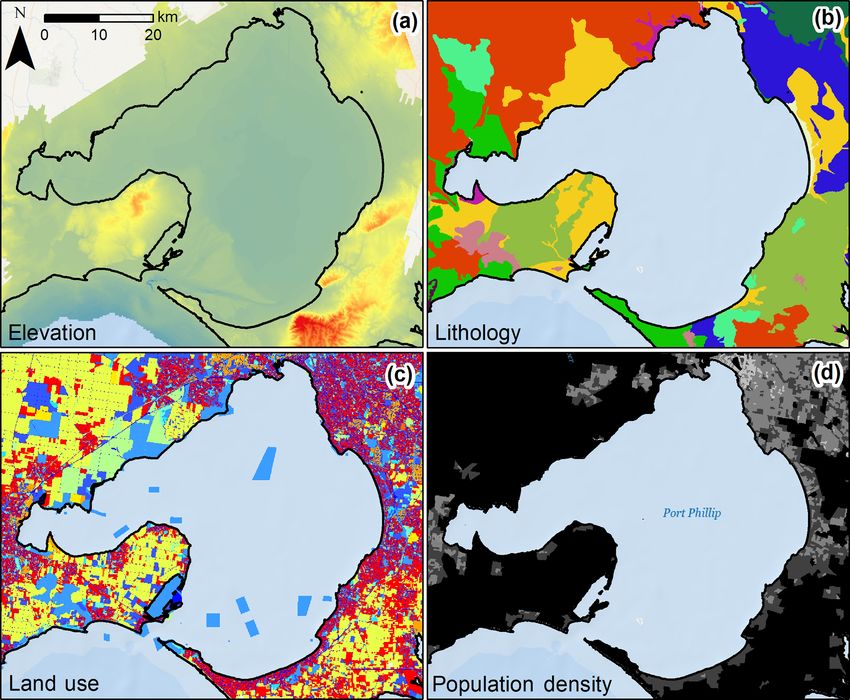
C. J. Ewers Lewis et al.: Drivers and modelling of blue carbon stock variability                                              2043

puts on sediment C stocks appears to be linked to three pos-        tied to human activities, particularly population density, agri-
sible mechanisms: (1) fluvial environments are usually as-          culture, and deforestation (Yang et al., 2003). Export of fine
sociated with smaller grain size sediments (silts and muds),        sediments to coastal ecosystems from eroded terrestrial soils
which can enhance C preservation by reducing sediment aer-          may encourage trapping and preservation of C within the sed-
ation compared to sandy sediments (Kelleway et al., 2016;           iments of blue C ecosystems.
Saintilan et al., 2013), (2) higher freshwater input may lead          Assessments of the drivers of blue C stock variability are
to higher plant biomass and therefore autochthonous C inputs        often completed at global scales (Atwood et al., 2017; Rovai
(Kelleway et al., 2016), and (3) there is a greater contribution    et al., 2018). Given the variability of sediment C stocks at
of terrestrial sediments via suspended particulate organic C        finer spatial scales and that coastal resources are managed
and suspended sediment concentration higher up in the catch-        on finer scales, we wanted to investigate drivers influencing
ment compared to near the coast (Van De Broek et al., 2016).        regional blue C sediment stock variability. Here, we had the
   Along with position in an estuary or catchment, proxim-          opportunity to exclude comparisons between temperate and
ity to freshwater inputs may drive differences in sediment C        tropical climates or effects of latitude by working on a stretch
stocks among and within ecosystem patches. Tidal marsh ac-          of coastline that spans approximately 1500 km west to east.
cretion rates, which have been positively correlated (87 %)         We tested the relationship between ecological, geomorpho-
with organic matter inventory, tend to decrease with distance       logical, and anthropogenic variables and sediment blue C
from freshwater channels (Chmura and Hung, 2004), sug-              stocks in the mineral-dominated sediments of southeastern
gesting sediment C stocks may be higher closer to channels.         Australia. By identifying drivers of small-scale variability in
Distance to freshwater is positively correlated with surface        sediment C stocks, across and within ecosystem patches, we
elevation, suggesting areas further from channels are inun-         created a predictive model for estimating C stocks on a scale
dated less frequently and thus have less sedimentation and          relevant to coastal resource management. Our specific objec-
slower accretion rates (Chmura and Hung, 2004).                     tives were to (1) identify ecological, geomorphological, and
   It is important to note that high sedimentation rates do not     anthropogenic factors driving variability in 30 cm deep sed-
necessarily result in high C sequestration rates or stocks if in-   iment blue C stocks within and across ecosystem patches in
organic sediments make up a substantial portion of new sedi-        southeastern Australia; (2) produce a spatially explicit model
ment composition. Finer particles have higher surface area to       of current 30 cm deep sediment blue C stocks based on the
volume ratios and tend to bind more organic molecules than          relative importance of environmental drivers in southeastern
coarse particles (Mayer, 1994). In seagrasses, high mud con-        Australia; and (3) map regional 30 cm deep sediment blue C
tent is correlated with high sediment organic C content, ex-        stock magnitude and variability.
cept when large autochthonous inputs (e.g. seagrass detritus
from large species such as those of Posidonia and Amphibolis
genera) disrupt this correlation (Serrano et al., 2016a).           2     Materials and methods
   Anthropogenic activities may also influence the C sink ca-
pacity of blue C ecosystems, even when the sediments are            2.1    Sediment C stock dataset
not directly disturbed (Lovelock et al., 2017). Land use, par-
ticularly in areas dominated by farmland and urbanization,          Sediment C stocks to 30 cm deep were estimated for 287
has been associated with worsening of seagrass condition, in-       sediment cores from 96 blue C ecosystems across Victoria
cluding abundance and species richness (Quiros et al., 2017),       in southeastern Australia (Ewers Lewis et al., 2020; Ewers
which may result in impacts on sediment C stocks. Nutrient          Lewis et al., 2018; Fig. 1). Full details of sample collec-
additions resulting from agriculture and urbanization may           tion, laboratory analyses, and calculations of C stocks can
increase primary productivity in nutrient-limited areas (Ar-        be found in Ewers Lewis et al. (2018). Briefly, three repli-
mitage and Fourqurean, 2016). However, reduced nutrient             cate sediment cores (5 cm inner diameter) were taken in each
inputs to coastal ecosystems could benefit C sequestration,         ecosystem (n = 125 in tidal marsh, n = 60 in mangroves, and
as nutrient additions can result in net C loss through plant        n = 102 in seagrasses). Once back in the laboratory, samples
mortality, erosion, efflux, and remineralization via enhanced       were taken from three depths (0–2, 14–16, and 28–30 cm)
microbial activity (Macreadie et al., 2017b). Further, excess       within each core. Samples were dried at 60◦ until a consis-
N has been linked to enhanced decomposition and an overall          tent weight was achieved and then ground. Dry bulk density
increase in tidal marsh ecosystem respiration due to shifts in      (DBD) was calculated as the dry weight divided by the orig-
microbial communities (Kearns et al., 2018).                        inal volume for all samples.
   Land use and human population may also impact blue C                Based on the protocols by Baldock et al. (2013), a combi-
sediment stocks through erosion of terrestrial soils. Human         nation of diffuse reflectance Fourier transform mid-infrared
activities causing erosion on land can result in increased sed-     (MIR) spectroscopy and elemental analysis via oxidative
iment loads to coastal areas, including fine particles with a       combustion using a LECO Trumac CN analyser was used to
high affinity for C (Mazarrasa et al., 2017; Serrano et al.,        determine organic C contents of all samples. Previous stud-
2016b). An average of 60 % of global soil erosion has been          ies have demonstrated the accuracy of using MIR to esti-

www.biogeosciences.net/17/2041/2020/                                                       Biogeosciences, 17, 2041–2059, 2020
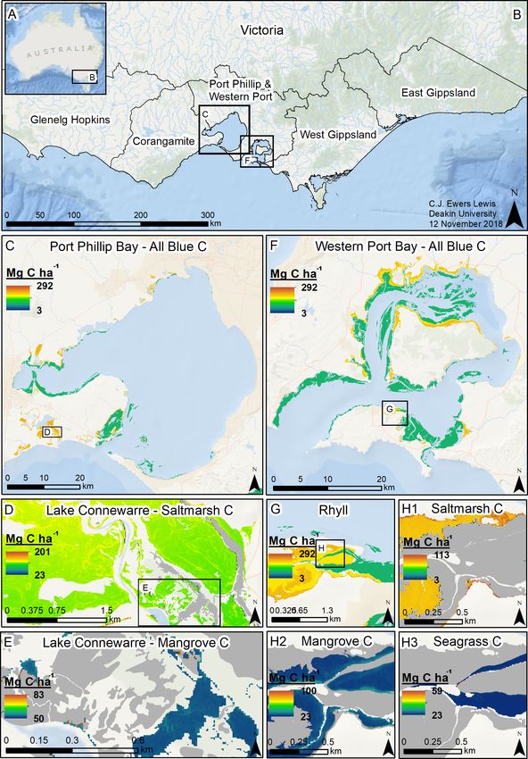
2044                                         C. J. Ewers Lewis et al.: Drivers and modelling of blue carbon stock variability

Figure 1. Sample locations for 30 cm deep sediment blue C stock measurements across Victoria, Australia (a), focusing in on Port Phillip
and Western Port bays (b). Service layer credits: Esri, Garmin, GEBCO, NOAA NGDC, and other contributors. Adapted from Ewers Lewis
et al. (2018).

mate organic C stocks of sediments (Baldock et al., 2013;             densities for each interval (measured and extrapolated) were
Van De Broek and Govers, 2019; Ewers Lewis et al., 2018).             summed and converted to Mg C ha−1 to estimate total stock
MIR spectra were acquired for all samples, and a subset of            down to 30 cm deep for each core location.
200 representative samples was selected based on a prin-                 Though it is common in the literature to sample to 1 m
cipal components analysis (PCA) of the MIR results uti-               deep in blue C sediments, the sampling protocol used for col-
lizing the Kennard-Stone algorithm. Gravimetric contents              lecting these data (Ewers Lewis et al., 2018) was designed to
of organic carbon were measured directly in the laboratory            maximize spatial coverage of sediment C samples rather than
for the 200-sample subset (Baldock et al., 2013). A partial           sample entire sediment profiles (which may extend well be-
least-squares regression (PSLR) was created using a Ran-              yond 1 m deep). Greater spatial coverage allowed us to test
dom Cross-Validation Approach (Unscrambler 10.3, CAMO                 the relationships between a variety of potential drivers and
Software AS, Oslo, Norway) and used to build algorithms               30 cm deep sediment C stocks on both fine and broad scales.
to predict square-root-transformed total carbon, total organic
carbon, total nitrogen, and inorganic carbon for the entire           2.2   Generation of predictor variables
dataset. The PSLR model was evaluated based on parame-
ters from the chemometric analysis of soil properties (Bellon-        Our general approach to identifying potential drivers of
Maurel et al., 2010; Bellon-Maurel and McBratney, 2011),              30 cm deep sediment C stock variability was to develop a
and the relationship between measured and predicted values            predictive model based on spatially explicit environmental
was assessed based on slope, offset, correlation coefficient          factors associated with our high spatial density of sediment
(r), R 2 , the root-mean-square error (RMSE), bias, and stan-         C sampling. For clarity, we have grouped predictor variables
dard error (SE) of calibration (SEC) and validation (SEP; see         into three categories – ecological, anthropogenic, and geo-
Ewers Lewis et al., 2018 for full details). R 2 for all square-       morphological – though the processes impacting C storage
root-transformed variables was ≥ 0.94.                                for each may span all three categories (Tables 1, S1 in the
   Sediment C stocks were calculated based on Howard et               Supplement).
al. (2014). Organic C density (mg C cm−3 ) was calculated by             Values of predictor variables for each core were deter-
multiplying organic C content (mg C g−1 ) by DBD (g cm−3 ).           mined from spatial data either as the collective value rep-
Linear splines were applied to each core to estimate C den-           resenting activities within the catchment or based on the ex-
sity for each 2 cm increment within the 30 cm core, then C            act location of sample collection, depending on the variable.
                                                                      Geographical boundaries for catchments in Victoria were de-

Biogeosciences, 17, 2041–2059, 2020                                                         www.biogeosciences.net/17/2041/2020/
C. J. Ewers Lewis et al.: Drivers and modelling of blue carbon stock variability 2045 rived using high-resolution elevation data and flow accumu- Area” tool was used in ArcMap based on the catchment re- lation models to define the spatial extents influencing fluvial gion polygons. From the total area of each lithology in each and estuarine catchments (Barton et al., 2008; Fig. S1 in the catchment, the one with the greatest proportion was identi- Supplement). In some instances, seagrass locations sampled fied and input into a new field from which a new primary were beyond fluvial and estuarine catchments defined, thus lithology raster was created. The Extract Values to Points we allocated characteristics of the nearest catchment region tool in ArcMap was used to extract primary lithology raster to characterize catchment influences at these locations. values to each sample location. In total, 21 lithologies were Plant community was defined in two ways. First, more identified in the dataset, 17 of which were identified as pri- generally as “ecosystem” (mangrove forest, tidal marsh, or mary lithologies of the coastal catchments (Table S2). seagrass meadow) based on the plant cover where the sam- Variables to assess the influence of anthropogenic pro- ple was taken. Second, plant communities were further de- cesses on 30 cm deep sediment blue C stocks included three fined by either dominant species (for seagrasses, for which relating to land use and one relating to human population. most were monotypic beds) or ecological vegetation class Primary land use for the catchment was first defined as the (EVC; for tidal marshes); for clarity, classification by either primary land use (based on land use in individual poly- dominant species or EVC will be referred to as EVC from gons) covering the greatest proportion of the catchment area. here on out. EVC was determined for each sampling location Land use spatial data were obtained from the Victorian Land based on percentage cover of 1 m2 quadrat photos taken dur- Use Information System (2014/2015) from the Victoria State ing sample collection. Tidal marsh EVCs sampled included Government, Department of Economic Development, Jobs, coastal tussock saltmarsh, wet saltmarsh herbland, and wet Transport and Resources. In total, nine general primary land saltmarsh shrubland, as described by Boon et al. (2011). use categories were identified in the dataset, all of which Only one mangrove species is present in Victoria (the grey were identified as primary land uses of the coastal catch- mangrove, Avicennia marina); therefore, further classifica- ments (Table S3). The nine land use categories were pooled tion of this ecosystem was not used. Seagrass species sam- into three simplified categories: urbanized, agricultural, and pled included Lepilaena marina, Posidonia australis, Ruppia natural. Then the areas of each within the catchment were megacarpa, Zostera muelleri, and Zostera nigricaulis. summed and divided by total catchment area to provide the Topographical variables for each sample location included proportion of each catchment associated with those cate- elevation and slope. Elevation data were obtained from the gories. Victorian Coastal Digital Elevation Model 2017 from the Co- Human population densities were calculated for each operative Research Centre for Spatial Information. Elevation catchment based on 2011 Australian census data, which were data at 2.5 m spatial resolution were used where available. the most recent data available (Table S1). Population density Where not available (for 2.8 % of cores), 10 m spatial reso- was calculated for each district by dividing the population of lution elevation data were used to fill in the gaps. Slope was the district by the area; this was then converted to a raster calculated from these data using the “Slope” tool in ArcMap (100 m2 resolution) to calculate the mean population density (v. 10.2.2 for desktop). The elevation data are a composite for the area of each catchment. product that integrated terrestrial and bathymetric lidar as Complete details of data availability for inputs and outputs well as multi-beam sonar data. The vertical accuracies of the of our models can be found in Table S10. data varied with sensor setup for acquisition: ±10 cm at 1 sigma (68 % conf. level) in bare ground for topographic lidar 2.3 Model generation, selection, averaging, and data (for the majority of our dataset), ±50 cm for bathymet- validation ric lidar, and ±
2046                                          C. J. Ewers Lewis et al.: Drivers and modelling of blue carbon stock variability

Figure 2. Variability of select potential C stock drivers in Port Phillip Bay, Victoria, Australia. Raw spatial data layers were processed to
define covariate values at each sample location or for the catchment of the sample location. Pictured layers include (a) elevation raster at
10 m resolution, (b) lithology polygons, (c) land use polygons, and (d) population density polygons.

els containing all possible variables (“global” models, as ex-           for mapped blue C ecosystems in Victoria. R code for this
plained below) using AICC (Akaike information criteria, cor-             project can be found in the Harvard Dataverse (Ewers Lewis
rected for small sample size) to explain the variability ob-             and Young, 2020).
served in the training dataset (70 % of total C stock data;                 To begin this process, potential ecological, geomorpholog-
Symonds and Moussalli, 2011). From there, we identified                  ical, and anthropogenic drivers were identified from the lit-
which variables within the best global models best explained             erature, and relevant proxies were extracted from available
the observed variability in C stock data in order to remove              spatial data using ArcMap (Tables 1; S1). Predictor variable
unnecessary variables from the model equation (through the               values derived from spatial data (along with our response
process of “dredging” and selecting the best subset, ex-                 variable values of C stocks) were compiled into a master data
plained in detail below). The validity of removing unnec-                table in ArcMap. Sample rows were randomly assigned as ei-
essary variables from the model is supported by the con-                 ther “training” data to build the model (70 % of the data) or
cept of parsimony, which suggests that models more compli-               “evaluating” data with which to validate the model (the re-
cated than the best model provide little benefit and should be           maining 30 % of the data). The training dataset was imported
eliminated (Burnham and Anderson, 2002; Richards, 2008).                 into R (R Core Team, 2018) for further analysis.
The best subset of models generated from the global models                  Covariates were tested for correlation before composing
(“dredge products”) were selected based on delta AICC
C. J. Ewers Lewis et al.: Drivers and modelling of blue carbon stock variability                                                2047

Figure 3. Conceptual workflow of sediment C stock modelling methods: preparation, model creation and selection, model averaging, vali-
dation, and predictions.

agricultural, Fig. S2). This resulted in four variables that did     along with one covariate each from the ecological and an-
not correlate with other covariates and could be used together       thropogenic variable groups, resulting in 12 global models
in all models (slope, distance to coast, distance to freshwa-        containing 6 covariates each (Table S4). Continuous covari-
ter, and primary lithology – hereafter referred to as “geo-          ates were scaled in R. Site (i.e. a single sampling area that
morphological covariates”), along with correlating covariates        contained from one ecosystem up to all three ecosystems)
that fell into one of two groupings: (1) ecosystem, EVC, and         was used as a random effect in all models to account for spa-
elevation were correlated (hereafter referred to as “ecologi-        tial autocorrelation observed at ∼ 78 km.
cal covariates”, and (2) mean population density, proportion            The 12 global models were ranked using AICC (AICcmo-
urbanized land use, proportion agricultural land use, and pro-       davg package v. 2.1–1; Mazerolle, 2017; Table S5). The four
portion natural land use were correlated (hereafter referred to      best global models were chosen for further analysis based
as “anthropogenic covariates”).                                      on delta AICC ≤∼ 5.0 compared to >30 for all other mod-
   As a first step, we aimed to identify which models that in-       els. Because the top four global models all used EVC as the
cluded all (non-correlated) variables were best for explaining       ecological variable, this process was repeated for the next
the variability in C stock data. Global models (i.e. containing      four best models – those that included ecosystem as the eco-
all possible variables) were created and ranked to identify the      logical predictor – to create averaged models that could be
most important drivers of C stock variability. General linear        tested and used for predictions when more specific, spatially
mixed-effects models (GLMMs) were generated (family =                explicit plant community data (i.e. EVC) were not available.
gamma, as our data were right-skewed; lme4 package v. 1.1–              The eight global models were “dredged” (MuMIn pack-
17; Bates et al., 2015) using all geomorphological covariates,       age v. 1.42.1; Barton, 2018) to assess the relative importance

www.biogeosciences.net/17/2041/2020/                                                         Biogeosciences, 17, 2041–2059, 2020
2048                                          C. J. Ewers Lewis et al.: Drivers and modelling of blue carbon stock variability

Table 1. Hypothesized drivers of 30 cm deep sediment blue C stock variability. Drivers were grouped into three categories: (1) ecological
(ecosystem type and dominant species or EVC), (2) geomorphological (elevation, slope, distance to freshwater channel, distance to coast,
and lithology), and (3) anthropogenic (land use and population). A more detailed explanation of driver rationale, along with literature and
spatial data references, can be found in Table S1.

     Driver                            Hypothesis and rationale
     Ecological
     Ecosystem type                    Ecosystem is the dominant driver of C stock variability. C stocks differ by ecosystem type due to
                                       (1) differences in position in the tidal frame and (2) differences in morphology, which influence
                                       settling and trapping of suspended particles, as well as production of autochthonous C inputs.
     Ecological vegetation class       Species composition better explains C stock variability than ecosystem alone. C stocks vary
                                       across species and community composition, as well as elevation.
     Geomorphological
     Elevation                         Lower elevations are correlated with higher C stocks. Lower elevations have higher
                                       sedimentation rates, aiding the trapping of organic C, and are inundated more often, providing
                                       more opportunity for contribution of allochthonous C.
     Slope                             Shallower slopes are correlated with higher C stocks. Steeper slopes are more vulnerable to
                                       erosion and less conducive to sedimentation and particle trapping than shallower slopes.
     Distance to freshwater channel    Distance to freshwater channel is negatively correlated with C stocks. Being in close proximity
                                       to freshwater inputs may increase plant growth via freshwater and nutrient inputs and enhance
                                       C preservation through delivery of smaller grain size particles.
     Distance to coast                 C stocks are greater higher up in the catchment. Greater inputs of organic C from terrestrial
                                       sources higher in the catchment result in higher sediment C stocks.
     Lithology                         C stocks vary with terrestrial parent material of sediments. Rock type may influence grain size
                                       and mineral content of sediments exported from catchments; smaller grain sizes and certain
                                       minerals enhance C stocks and preservation.
     Anthropogenic
     Land use                          C stocks vary based on land use activities in the catchment. Export of terrestrial C, nutrients, and
                                       sediments varies by land use, especially when comparing urbanized, agricultural, and natural
                                       land uses.
     Population density                C stocks differ across population levels due to a correlation with land use.
                                       Increases in population size lead to increases in urbanization and competition for land use.

of covariates included in each model. In this context, dredg-               Averaged models were validated using the 30 % evalua-
ing refers to the generation of a set of models that includes            tion dataset. Due to the limitations of using cross-validation
all possible combinations of fixed effects from the global               and bootstrapping on models with random effects (Colby and
model, containing from six to one variables (i.e. all combi-             Bair, 2013), a direct comparison was done between predicted
nations of five variables, all combinations of four variables,           and actual values of the reserved dataset. The “predict” func-
and so on). The dredge products of each global model (i.e.               tion in R was used to generate predicted C stock values for
models created from dredging) were ranked using AICC and                 30 cm deep sediments using each of the eight averaged mod-
the best models (delta AICC
C. J. Ewers Lewis et al.: Drivers and modelling of blue carbon stock variability 2049
(ANOVA) was run using EVC as the factor. A Tukey’s mean population density, and proportion agricultural land
post hoc analysis was used to distinguish groupings. use.
Dredging the top four global models and averaging the
2.4 Prediction of 30 cm deep sediment blue C stocks best dredge products (delta AICC2050 C. J. Ewers Lewis et al.: Drivers and modelling of blue carbon stock variability Table 2. Parameter estimates for averaged models containing ecological vegetation class (EVC) as the ecological variable. Parameter esti- mates were calculated based on averaging the best model products (delta AICC
C. J. Ewers Lewis et al.: Drivers and modelling of blue carbon stock variability                                                       2051

Table 3. Parameter estimates for averaged models containing ecosystem as the ecological variable. Parameter estimates were calculated
based on averaging the best model products (delta AICC
2052                                           C. J. Ewers Lewis et al.: Drivers and modelling of blue carbon stock variability

Figure 5. Modelled 30 cm deep sediment blue C stocks for Victoria, Australia. Location of Victoria in Australia (a); coastal catchment regions
of Victoria (b); modelled C stocks for all blue C ecosystems in Port Phillip Bay (c); modelled saltmarsh C stocks in Lake Connewarre (d);
modelled mangrove C stocks in subsection of Lake Connewarre (e); modelled C stocks for all blue C ecosystems in Western Port Bay
(f); modelled C stocks for all blue C ecosystems in Rhyll (Phillip Island) (g); and modelled saltmarsh C stocks (h1), mangrove C stocks
(h2), and seagrass C stocks (h3) in a subsection of Rhyll. Base map service layer credits: Esri, Garmin, GEBCO, NOAA NGDC, and other
contributors.

more important driver in C accumulation variability than the             fects of elevation compared to vegetation community could
difference in biomass production between the two ecosys-                 not be teased apart without violating assumptions of non-
tems (Saintilan et al., 2013), highlighting the importance of            collinearity in our models. However, the higher ranking of
elevation in determining C stocks. In our study, elevation               global models with EVC or ecosystem above those with el-
was correlated to ecosystem and EVC, thus the differing ef-              evation in our study suggests that the plant community itself

Biogeosciences, 17, 2041–2059, 2020                                                             www.biogeosciences.net/17/2041/2020/
C. J. Ewers Lewis et al.: Drivers and modelling of blue carbon stock variability                                                                                     2053

Table 4. Blue C ecosystem area (ha) and modelled 30 cm deep sediment C stocks (Mg C) by catchment region and total across the state
(Victoria, Australia). N/A signifies that no ecosystem extent is reflected in recent mapping in these catchment regions; therefore, C stock
measurements could not be scaled up or modelled by ecosystem area.

                                              Tidal marsh                         Mangrove                         Seagrass             All blue C ecosystems in Victoria
 Catchment region                     Area (ha)   C stocks (Mg C)     Area (ha)     C stocks (Mg C)    Area (ha)     C stocks (Mg C)    Total area (ha)     Total blue C
                                                                                                                                                           stock (Mg C)
 Glenelg Hopkins                           138                6828         N/A                  N/A         N/A                  N/A               170             6828
 Corangamite                             3010               187 943         58                 3022        5355               128 117            8423            319 083
 Port Phillip and Western Port bays      3108               158 604       1828                90 359      14 457              328 725           19 393           577 688
 West Gippsland                         13 038              711 083       3301               161 652      17 508              413 642           33 847         1 286 377
 East Gippsland                          1332                50 504        N/A                  N/A        5552                72 873            6884            123 377
 Total                                  20 626          1 114 961         5187               255 034      42 903              943 357           68 715         2 313 352

Table 5. Modelled 30 cm deep sediment blue C stocks (Mg C) by region of interest (ROI; listed from west to east). N/A: ecosystem does not
occur in ROI.

                                                                             C stocks (Mg C) by ecosystem
                      Region of interest                                 Tidal marsh          Mangrove       Seagrass                 All blue C
                                                                                                                              ecosystems in ROI
                      Breamlea                                                 18 650              N/A           N/A                        18 650
                      Lake Connewarre/Barwon Heads                            101 218             2890           N/A                       104 109
                      Port Phillip Bay                                        105 169               243       156 824                      262 236
                      Western Port Bay                                        120 827            90 248       300 420                      511 495
                      Andersons Inlet                                          18 992             7455            890                       27 337
                      Shallow Inlet                                             9384               N/A         19 778                       29 162
                      Corner Inlet                                            253 367           154 198       346 317                      753 882
                      Jack Smith Lake                                          73 839              N/A           N/A                        73 839
                      Lake Denison                                              7353               N/A           N/A                         7353
                      Gippsland Lakes                                         391 023              N/A         99 267                      490 291
                      Lake Corringle                                            3449               N/A           N/A                         3449
                      Bemm River region                                          N/A               N/A          7806                         7806
                      Tamboon Inlet                                              N/A               N/A          2563                         2563
                      Wallagaraugh River/Mallacoota region                      3180               N/A          8117                        11 296
                      Total                                                 1 106 452           255 034       941 982                   2 303 468

is a better predictor of 30 cm deep sediment C stocks than                                 Geomorphological variables were more important than
simply position in the tidal frame.                                                     most anthropogenic variables in our models (Tables 2 and
   Our global models specifying dominant species (for sea-                              3). Though lithology was not part of our averaged models, it
grass meadows) or EVC (for tidal marshes) ranked higher in                              is possible that its exclusion was due mostly to scale (catch-
our model selection than those that only specified the ecosys-                          ment) and that it may be important when accounted for on
tem (i.e. tidal marsh, mangrove, or seagrass). This ranking                             a more local scale. Distance to coast, distance to freshwa-
was supported by our model validation, in which our aver-                               ter channels, and slope all appeared in the averaged mod-
aged model that best explained 30 cm deep sediment C stock                              els using EVC, with distance to coast being most important.
variability included EVC and accounted for 48.8 % of the                                However, in models using ecosystem, distance to freshwater
variability observed (Fig. S3). Still, the best averaged model                          channels was no longer important enough to appear in the
containing ecosystem as the ecological predictor performed                              averaged models, and the anthropogenic variables, propor-
nearly as well and explained 46.2 % of the variability. These                           tion urbanized and proportion natural, were more important
results suggest that even when specific data on species com-                            than any of the geomorphological variables. Model valida-
position are not available, 30 cm deep sediment C stocks can                            tion revealed that the best predictions for either set of models
be estimated with a similar degree of confidence based on                               (those using EVC and those using ecosystem as the ecolog-
ecosystem type, which is often a much more readily avail-                               ical variable) came from the model that did not include any
able form of data and therefore favourable for calculating                              anthropogenic variables.
sediment C stocks in data-deficient areas.

www.biogeosciences.net/17/2041/2020/                                                                                    Biogeosciences, 17, 2041–2059, 2020
2054 C. J. Ewers Lewis et al.: Drivers and modelling of blue carbon stock variability
Although our models suggest anthropogenic variables Ecosystem type was a relatively powerful predictor of
have little impact on 30 cm deep sediment C stocks, it is more 30 cm deep sediment C stock variability in our study and this
likely that anthropogenic variables are impacting processes is likely due, in part, to the direct relationship between vege-
we could not measure. For example, excess nutrients result- tation and surface sediments. In most vegetated ecosystems,
ing from certain land uses may stress plants to the point of af- the majority of underground plant biomass and microbial ac-
fecting survival and therefore sediment stability (Macreadie tivity exists within the top 20 cm of soils (Trumbore, 2009).
et al., 2017b). Without measuring changes to ecosystem dis- For saltmarsh, it has been demonstrated that the top 30 cm of
tribution or sediment thickness (i.e. erosion), we could not sediment are directly impacted by current vegetation (Owers
pick up on these sediment C losses. Similarly, though en- et al., 2016). Therefore, using 30 cm deep sediment C stock
hanced sedimentation rates may increase C burial in catch- measurements allowed us to target the portion of the sedi-
ments with certain land uses (e.g. high population density or ment profile most likely to be influenced by current vegeta-
high area of agriculture; Yang et al., 2003), this addition to C tion.
stocks would be reflected in sequestration rate, which we did The portion of recently accreted sediments influenced by
not measure in this study. contemporary anthropogenic drivers is harder to identify than
Proxies for the drivers of sediment C stock variability can that influenced by ecosystem vegetation. Based on estimated
be quantified and described for modelling in numerous ways. accretion rates for this region from the literature (Ewers
Though we maximized our ability to choose variables repre- Lewis et al., 2019; Rogers et al., 2006b), 30 cm deep sedi-
senting meaningful relationships with 30 cm deep sediment ments would have taken an average of ∼ 80 years to accumu-
C stocks by alternating the forms of the anthropogenic vari- late in Victoria (∼ 117 years in tidal marsh and ∼ 42 years
ables tested in our models (i.e. proportion urban vs. propor- in mangroves). Though sedimentation rates vary over time,
tion agriculture vs. proportion natural vs. mean population they are relatively steady in comparison to changes in an-
density), it may be beneficial to incorporate more direct mea- thropogenic drivers, such as land use change, which can hap-
sures of anthropogenic impacts in C stock modelling, such as pen abruptly. This means that modern-day maps of land use,
nutrients and suspended particulate organic matter coming though useful for looking at the general impact of human ac-
from catchments. tivities on ecosystem processes, may be more useful for re-
We also aimed to maximize our ability to capture relation- lating to variability in sediment C stocks when the data are
ships between contemporary drivers and sediment C stocks assessed at finer temporal resolutions. For example, compar-
by utilizing sediment C stock data to only 30 cm deep, a ing land use area data across various time periods with C
sediment horizon more directly impacted by recent environ- densities in aged bands of sediment could help capture the
mental conditions compared to deeper stocks due to age. pulse effects of sudden land use changes in narrower sed-
Based on previously estimated sediment accretion rates in iment horizons representative of the same time periods. In
blue C ecosystems in the study region (averaging 2.51 to this study, the effects of land-use change may have been too
2.66 mm yr−1 in tidal marshes, Ewers Lewis et al., 2019; diluted within the 30 cm horizons to relate to impacts on sed-
Rogers et al., 2006a; and 7.14 mm yr−1 in mangroves, Rogers iment C stock.
et al., 2006a), the top 30 cm of sediment represents roughly Spatially, anthropogenic variables are also difficult to as-
∼ 113–120 years of accretion in Victorian tidal marshes sign to particular ecosystem locations or depths. Many blue
and ∼ 42 years of accretion in Victorian mangroves. These C ecosystems in Victoria are located in coastal embayments
timescales suggest sediments depths utilized in this study are and receive inputs from multiple catchments, making the in-
more appropriate for assessing the impacts of modern en- fluence of specific areas of land-use or population changes
vironmental conditions on sediment C stocks compared to difficult to track to specific ecosystem locations. Modern-day
metre-deep stocks, which can be thousands of years old (e.g. factors influencing vegetation can also have impacts on C
Ewers Lewis et al., 2019). Using 30 cm deep sediment C stocks deeper than the sediments we measured. The effects
stocks also allows us to be more confident that the vegetation of underground biomass on sediment C stocks can extend
present now has been there during the time of sediment ac- beyond the top 30 cm, and in fact new C inputs and active
cretion, unlike deeper sediments that are thousands of years C cycling by microbial communities can occur as deep as
old and for which it is difficult to determine what vegetation, underground roots extend (Trumbore, 2009). These new C
if any, was present at the time of accretion. additions (and fluxes) at depth fall outside the general pat-
The variability in 30 cm deep sediment C stocks that could tern of sediment C decay down-core in vegetated ecosystems
not be explained by our modelling may also be related to the (Trumbore, 2009), which has previously allowed for linear or
inherent challenges surrounding spatial and temporal match- logarithmic regressions to be used to extrapolate 1 m deep C
ing of driver proxies and sediment C stock measurements; the contents from shallow (e.g. 30–50 cm deep) sediment C data
relationship between 30 cm deep sediment C stocks and con- (Macreadie et al., 2017a; Serrano et al., 2019). The activity
temporary environmental settings can be represented more of underground biomass and microbes at depth, when con-
accurately for some variables over others. sidered over space and time, may account for large C fluxes.
The influence of anthropogenic activities, such as land use
Biogeosciences, 17, 2041–2059, 2020 www.biogeosciences.net/17/2041/2020/C. J. Ewers Lewis et al.: Drivers and modelling of blue carbon stock variability 2055
changes, on these processes via impacts to vegetation may of total 30 cm deep sediment blue C stocks (Ewers Lewis et
largely go unnoticed based on current methods (Trumbore, al., 2018). Our original estimate of mangrove contribution
2009), both in this study and in blue C stock assessments on to total blue C was supported by our modelling: by either
larger scales. We suggest further research to understand the method, we estimated mangroves to store 11 % of Victoria’s
dynamics of active C cycling at sediment depths traditionally 30 cm deep sediment blue C stocks.
considered stable. It is important to emphasize here that total sediment depths
Another limitation to C stock modelling is knowledge of in blue C ecosystems can vary greatly, and are commonly
environmental features that may be important in influencing deeper than 30 cm. Blue C ecosystems can have sediments
C storage but are generally not monitored. For example, the up to several metres deep (e.g. Lavery et al., 2013; Scott
maturity of a blue C ecosystem can affect C storage and com- and Greenberg, 1983), suggesting the estimates of C stocks
position (Kelleway et al., 2015). Within a single saltmarsh measured here are conservative. In spite of these limitations,
species, the maturity of the system is a major factor deter- 30 cm deep sediment C stock estimates give us valuable
mining the role of the marsh as a C sink. Mature systems of knowledge about the sediment C pool most vulnerable to
Spartina maritime have higher C retention – via higher below disturbance and how it may be impacted by environmental
ground production, slower decomposition rate, and higher drivers.
C content in sediments – than younger S. maritime marsh In examining C stocks within ROIs, i.e. areas of the coast
systems (Sousa et al., 2010b). Mature marshes have also containing substantial distributions of blue C ecosystems, we
been observed to have greater contributions of allochthonous found that just four of the 14 ROIs housed nearly 88 % of
C storage over time, while younger marshes predominantly 30 cm deep sediment blue C stocks in the state, a direct re-
have autochthonous organic matter signatures (Chen et al., flection of the large proportion of blue C ecosystem area in
2016; Tu et al., 2015). Long-term mapping of blue C ecosys- these regions (nearly 87 % of the state’s total blue C area).
tems could be beneficial for tracking maturity of vegetation This trend appears to be driven by the presence of extensive
for C stock modelling as well as reducing the error in C stock seagrass sediment C stocks (Table 5) in these four regions,
measurements associated with changes to blue C ecosystem accompanied by extensive tidal marsh sediment C stocks.
area. This result has important implications for management of
Finally, we suggest future studies examine the relationship coastal blue C. In cases where resources are limited, iden-
between the drivers we have described and individual blue C tification of areas housing major blue C sinks, in conjunction
ecosystem types in order to further refine sediment blue C with evaluation of other ecosystem services, can help provide
stock modelling. With a large dataset from a single ecosys- insight to guide conservation strategies. For example, strate-
tem, relationships may be identified that were overshadowed gies to conserve tidal marshes in the four major ROIs could
in this study by the inclusion of all three ecosystems. For ex- serve the additional purpose of helping to preserve the adja-
ample, because elevation correlated with our two ecological cent seagrass meadows via facilitation; tidal marshes serve
variables, it was not included in our best models. However, as filters of excess nutrients coming down from the catch-
within a single ecosystem, elevation may be an important ment (Nelson and Zavaleta, 2012) that may otherwise cause
driver of sediment C stock variability due to its relationship a loss of seagrass beds due to light reduction resulting from
with inundation regimes (Chen et al., 2016; Chmura et al., the growth of algal epiphytes, macroalgae, and phytoplank-
2003; Chmura and Hung, 2004). ton (Burkholder et al., 2007). Further, our mapping of within-
ecosystem-patch variability in 30 cm deep sediment C stocks
4.2 Modelled 30 cm deep sediment blue C stocks is an important output for facilitating management actions on
an applicable level, allowing prioritization of particular parts
Our estimate of 2.31 million Mg C stored in the top 30 cm of an ecosystem patch for conservation when necessary.
of sediment in all blue C ecosystems in Victoria was about
20 % lower than that of Ewers Lewis et al. (2018), who es-
timated 2.91 million Mg C based on the same C stock data 5 Conclusions
but calculated total stocks based on average C stock val-
ues and ecosystem extent in each of the five coastal catch- In this study, we had the unique opportunity to assess a large
ments. These results suggest that modelling 30 cm deep sed- regional dataset of 30 cm deep sediment blue C stocks to ex-
iment C stocks based on environmental drivers may reduce plore the influence of ecological, geomorphological, and an-
the chances of overestimating sediment C stocks by better ac- thropogenic variables in driving sediment blue C stock vari-
counting for fine-scale variability. Our modelled 30 cm deep ability. Because of the high spatial resolution of sampling
sediment C stock estimates support our earlier findings that within similar latitudes we were able to focus on variables
tidal marshes store more C than any other blue C ecosystem driving differences in 30 cm deep sediment C stocks within
in Victoria. Our estimates are now refined in that modelled catchments. We found that plant community was most impor-
stocks suggest tidal marshes store closer to 48 % (rather than tant for determining 30 cm deep sediment C stocks and that
53 %) and seagrasses store closer to 41 % (rather than 36 %) combining this variable with geomorphological variables re-
www.biogeosciences.net/17/2041/2020/ Biogeosciences, 17, 2041–2059, 20202056 C. J. Ewers Lewis et al.: Drivers and modelling of blue carbon stock variability
lating to position in the catchment allowed us to model stocks Review statement. This paper was edited by Steven Bouillon and
at a fine spatial resolution. Identification and mapping of reviewed by two anonymous referees.
these dense 30 cm deep sediment blue C sinks in Victoria,
in conjunction with evaluation of other ecosystem services,
will be useful for conservation management regionally, e.g.
References
through the identification of hotspots for protection and key
locations for restoration efforts. We recommend these meth- Armitage, A. R. and Fourqurean, J. W.: Carbon storage in sea-
ods be tested in other areas of the globe to determine whether grass soils: long-term nutrient history exceeds the effects of
they may be applicable for identifying relationships between near-term nutrient enrichment, Biogeosciences, 13, 313–321,
potential environmental drivers and sediment blue C stocks https://doi.org/10.5194/bg-13-313-2016, 2016.
and creating predictive sediment C stock models and maps Atwood, T. B., Connolly, R. M., Almahasheer, H., Carnell, P. E.,
for blue C ecosystems at scales relevant to resource manage- Duarte, C. M., Ewers Lewis, C. J., Irigoien, X., Kelleway, J. J.,
ment applications in other regions. Lavery, P. S., Macreadie, P. I., Serrano, O., Sanders, C. J., San-
tos, I., Steven, A. D. L., and Lovelock, C. E.: Global patterns in
mangrove soil carbon stocks and losses, Nat. Clim. Change, 7,
Data availability. The data associated with this study 523–528, https://doi.org/10.1038/NCLIMATE3326, 2017.
are accessible through the Harvard Dataverse: (1) sed- Baldock, J. A., Hawke, B., Sanderman, J., and MacDonald, L. M.:
iment carbon stock data (Ewers Lewis et al., 2020, Predicting contents of carbon and its component fractions in
https://doi.org/10.7910/DVN/6PFBO0), (2) R code (Ewers Australian soils from diffuse reflectance mid-infrared spectra,
Lewis and Young, 2020 https://doi.org/10.7910/DVN/0WKEHJ), Soil Res., 51, 577–595, https://doi.org/10.1071/SR13077, 2013.
and (3) blue carbon stock predictions map of Victoria, Australia Barton, J., Pope, A., Quinn, G., and Sherwood, J.: Identifying
(Ewers Lewis, 2020, https://doi.org/10.7910/DVN/UDOAUT). threats to the ecological condition of Victorian estuaries, Depart-
ment of Sustainability and Environment Technical Report, War-
rnambool, Victoria, 1–54, 2008.
Barton, K.: MuMIn: Multi-Model Inference, available at: https:
Supplement. The supplement related to this article is available on-
//cran.r-project.org/package=MuMIn, last access: 12 January
line at: https://doi.org/10.5194/bg-17-2041-2020-supplement.
2018.
Bates, D., Mächler, M., Bolker, B., and Walker, S.: Fitting Lin-
ear Mixed-Effects Models using lme4, J. Stat. Softw., 67, 1–48,
Author contributions. CJEL, DI, MAY, and PIM conceived the https://doi.org/10.18637/jss.v067.i01, 2015.
study. CJEL, JAB, BH, JS, PEC, and PIM produced the input carbon Bellon-Maurel, V. and McBratney, A.: Near-infrared (NIR) and
data for the model. CJEL and MAY wrote the code. CJEL analysed mid-infrared (MIR) spectroscopic techniques for assessing
the data, performed the calculations, and produced the GIS data and the amount of carbon stock in soils – Critical review and
maps. CJEL prepared the paper with contributions from all authors. research perspectives, Soil Biol. Biochem., 43, 1398–1410,
https://doi.org/10.1016/j.soilbio.2011.02.019, 2011.
Bellon-Maurel, V., Fernandez, E., Palagos, B., Roger, J., and
Competing interests. The authors declare that they have no conflict McBratney, A.: Prediction of soil attributes by NIR/MIR spec-
of interest. troscopy. Coming back to statistics fundamentals to improving
prediction accuracy, Trends Anal. Chem., 29, 1073–1081, 2010.
Boon, P. I., Allen, T., Brook, J., Carr, G., Frood, D., Harty, C., Hoye,
Acknowledgements. We thank Parks Victoria and the Victo- J., Mcmahon, Andrew Mathews, S., Rosengren, N., Sinclair, S.,
rian Coastal Catchment Management Authorities (CMAs) for their White, M., and Yugovic, J.: Mangroves and coastal saltmarsh of
support and funding: Marty Gent and Glenelg Hopkins CMA, Victoria: distribution, condition, threats and management, Insti-
Chris Pitfield and Corangamite CMA, Emmaline Froggatt and tute for Sustainability and Innovation, Victoria University, Mel-
Port Phillip Western Port CMA, Belinda Brennan and West Gipp- bourne, 2011.
sland CMA, and Rex Candy and East Gippsland CMA. Car- Bouillon, S., Dahdouh-Guebas, F., Rao, A. V. V. S., Koedam, N.,
olyn J. Ewers Lewis also thanks the University of Technology Syd- and Dehairs, F.: Sources of organic carbon in mangrove sedi-
ney for scholarship support. ments: variability and possible ecological implications, Hydro-
biologia, 495, 33–39, 2003.
Burkholder, J. M., Tomasko, D. A., and Touchette, B. W.: Sea-
Financial support. This research has been supported by Parks Vic- grasses and eutrophication, J. Exp. Mar. Biol. Ecol., 350, 46–72,
toria; the Victorian Coastal Management Authorities of Glenelg https://doi.org/10.1016/j.jembe.2007.06.024, 2007.
Hopkins, Corangamite, Port Phillip and Western Port, West Gipp- Burnham, K. P. and Anderson, D. R.: Model Selection and Mul-
sland, and East Gippsland; and the Australian Research Council timodel Inference: A Practical Information-TheoreticApproach,
(DECRA Fellowship no. DE130101084 and Linkage Project no. 2nd Edn., Springer, New York, 1–22, 2002.
LP160100242). Chen, S., Torres, R., and Goñi, M. a.: The Role of Salt Marsh Struc-
ture in the Distribution of Surface Sedimentary Organic Mat-
ter, Estuar. Coast., 39, https://doi.org/10.1007/s12237-015-9957-
z, 2016.
Biogeosciences, 17, 2041–2059, 2020 www.biogeosciences.net/17/2041/2020/You can also read