Year-round impact of winter sea ice thickness observations on seasonal forecasts - The Cryosphere
←
→
Page content transcription
If your browser does not render page correctly, please read the page content below
The Cryosphere, 15, 325–344, 2021
https://doi.org/10.5194/tc-15-325-2021
© Author(s) 2021. This work is distributed under
the Creative Commons Attribution 4.0 License.

Year-round impact of winter sea ice thickness observations on
seasonal forecasts
Beena Balan-Sarojini1 , Steffen Tietsche1 , Michael Mayer1,2 , Magdalena Balmaseda1 , Hao Zuo1 , Patricia de Rosnay1 ,
Tim Stockdale1 , and Frederic Vitart1
1 The   European Centre for Medium-Range Weather Forecasts, Shinfield Rd, Reading RG2 9AX, UK
2 Department   of Meteorology and Geophysics, University of Vienna, Vienna, Austria

Correspondence: Beena Balan-Sarojini (beena.sarojini@ecmwf.int)

Received: 17 March 2020 – Discussion started: 13 May 2020
Revised: 3 November 2020 – Accepted: 10 December 2020 – Published: 26 January 2021

Abstract. Nowadays many seasonal forecasting centres pro-         July and August, which is related to degraded initial condi-
vide dynamical predictions of sea ice. While initializing sea     tions during these months. Both ocean reanalyses, with and
ice by assimilating sea ice concentration (SIC) is common,        without SIT constraint, show strong melting in the middle
constraining initial conditions of sea ice thickness (SIT) is     of the melt season compared to the forecasts. This excessive
only in its early stages. Here, we make use of the availabil-     melting related to positive net surface radiation biases in the
ity of Arctic-wide winter SIT observations covering 2011–         atmospheric flux forcing of the ocean reanalyses remains and
2016 to constrain SIT in the ECMWF (European Centre for           consequently degrades analysed summer SIC. The impact of
Medium-Range Weather Forecasts) ocean–sea-ice analysis            thickness initialization is also visible in the sea surface and
system with the aim of improving the initial conditions of the    near-surface temperature forecasts. While positive forecast
coupled forecasts. The impact of the improved initialization      impact is seen in near-surface temperature forecasts of early
on the predictive skill of pan-Arctic sea ice for lead times of   freezing season (September–October–November) initialized
up to 7 months is investigated in a low-resolution analogue of    in May (when the sea ice initial conditions have been ob-
the currently operational ECMWF seasonal forecasting sys-         servationally constrained in the preceding winter months),
tem SEAS5.                                                        negative impact is seen for the same season when initial-
   By using winter SIT information merged from CS2 and            ized in the month of August when the sea ice initial con-
SMOS (CS2SMOS: CryoSat-2 Soil Moisture and Ocean                  ditions are degraded. We conclude that the strong thinning
Salinity), substantial changes in sea ice volume and thickness    by CS2SMOS initialization mitigates or enhances seasonally
are found in the ocean–sea-ice analysis, including damping        dependent forecast model errors in sea ice and near-surface
of the overly strong seasonal cycle of sea ice volume. Com-       temperatures in all seasons.
pared with the reference experiment, which does not use SIT          The results indicate that the memory of SIT in the spring
information, forecasts initialized using SIT data show a re-      initial conditions lasts into autumn, influencing forecasts of
duction of the excess sea ice bias and an overall reduction       the peak summer melt and early freezing seasons. Our re-
of seasonal sea ice area forecast errors of up to 5 % at lead     sults demonstrate the usefulness of new sea ice observational
months 2 to 5. Change in biases is the main forecast im-          products in both data assimilation and forecasting systems,
pact. Using the integrated ice edge error (IIEE) metric, we       and they strongly suggest that better initialization of SIT is
find significant improvement of up to 28 % in the Septem-         crucial for improving seasonal sea ice forecasts.
ber sea ice edge forecast started in April. However, sea ice
forecasts for September started in spring still exhibit a pos-
itive sea ice bias, which points to a melting that is too slow
in the forecast model. A slight degradation in skill is found
in the early freezing season sea ice forecasts initialized in

Published by Copernicus Publications on behalf of the European Geosciences Union.
326                          B. Balan-Sarojini et al.: Impact of winter sea ice thickness observations on seasonal forecasts

1   Introduction                                                    et al., 2014) in a dataset called CS2SMOS (Ricker et al.,
                                                                    2017).
                                                                       Currently SIC is the only sea ice variable assimilated in
Sea ice is an integral part of the Earth system as it regulates     the ECMWF ocean–sea-ice data assimilation system. Al-
the heat, moisture and momentum flux exchange between the           though the ECMWF sea ice reanalysis and reforecasts com-
polar oceans and the atmosphere. Decline in Arctic sea ice is       pare well with other systems (Chevallier et al., 2017; Uotila
a visible indicator of the changing climate. Forecasting Arc-       et al., 2019; Zampieri et al., 2018, 2019), they are affected
tic sea ice has advanced significantly in the last decade, with     by noticeable errors (Tietsche et al., 2018). There are large
most forecasting centres using prognostic sea ice models op-        biases in sea ice forecasts from months to seasons, pointing
erationally, allowing us to explore the sea ice forecast skill on   to uncertainties in both the models and observations used in
long lead times from weeks to months to seasons. Possibili-         the assimilation and forecasting systems. Here we explore
ties of economically viable shorter shipping routes across the      the pathway to improve the initialization using observations
Arctic in the summer are constantly being explored. Monthly         of sea ice thickness, which covers both the thick- and thin-
and seasonal outlooks of sea ice products are therefore in          ice regions of the Arctic. We then assess the impact of the
great demand especially by the Arctic communities, as well          changed sea ice initial condition on the forecast skill on long
as maritime and resource extraction industries.                     lead times of months to seasons. Compared to Blockley and
   Moreover, there is increasing scientific evidence that           Peterson (2018), who looked only at summer forecast skills,
warming and sea ice loss in the Arctic due to climate change        our study for the first time assesses the forecast impact of
affect the European weather and climate (Balmaseda et al.,          SIT initialization on all seasons using a fully coupled sea-
2010; Mori et al., 2014; Overland et al., 2016; Ruggieri et al.,    sonal forecasting system. We use the ECMWF coupled en-
2016). Unlike sea ice concentration and extent, long records        semble seasonal forecasting system SEAS5 and CS2SMOS
of satellite observations of sea ice thickness are sorely lack-     thickness observations.
ing (Laxon et al., 2003; Kwok and Rothrock, 2009; Haas                 Our study takes a forecasting system end-to-end perspec-
et al., 2010; Meier et al., 2014; Sallila et al., 2019; Scarlat     tive, from observations and modelling to forecast products.
et al., 2020).                                                      The rest of the article is organized as follows. Section 2 de-
   Since reliable estimates of long-term, basin-wide sea ice        scribes the methodology of sea ice thickness initialization
extent and volume are needed for understanding climate              and forecasting, including a brief description of ocean–sea-
change and for initializing numerical weather forecasts, there      ice models, the assimilation system, the atmosphere-ocean–
is growing interest in using improved and new types of sea          sea-ice coupled forecasting system, observations used and
ice observations in data assimilation systems (Lindsay et al.,      the experimental set-up. Section 3 presents the main results
2008; Blanchard-Wrigglesworth et al., 2011; Tietsche et al.,        and has three main foci: (i) assessing the impact of new SIT
2013; Sigmond et al., 2013; Balmaseda et al., 2015). Ear-           observations on the analysed sea ice state and the impact of
lier studies propose that long-term memory in the winter sea        the changed sea ice initialization on seasonal range sea ice
ice thickness can potentially improve summer sea ice extent         forecasts (Sect. 3.1 and 3.2), (ii) improving Arctic sea ice
forecasts (Guemas et al., 2016; Tietsche et al., 2014; Day          forecast skill by understanding the errors in the coupled fore-
et al., 2014). They concluded that potential predictability         cast model and the data assimilation system through targeted
mainly originates from the persistence or advection of sea ice      diagnostics (Sect. 3.3), and (iii) quantifying the impact of sea
thickness anomalies, interaction with ocean and atmosphere,         ice improvements on seasonal forecasts of atmospheric vari-
and changes in the radiative forcing.                               ables (Sect. 3.4). Finally, Sect. 4 provides the summary of the
   While assimilation of sea ice concentration (SIC) is rou-        findings with concluding remarks.
tinely done in operational sea ice forecasting, assimilation of
sea ice thickness (SIT) is at its early stages (Allard et al.,
2018; Xie et al., 2018; Mu et al., 2018; Fritzner et al., 2019).    2   Observations and methods
These studies have found that SIT initialization improves
sea ice forecasts in forced ocean–sea-ice forecasting sys-          The procedure followed here to assess the impact of SIT
tems which were run for short time periods spanning from            information follows a twin experiment approach. Each of
3 months up to 3 years. Blockley and Peterson (2018) re-            the experiments consists of two distinctive steps: (1) the
ported for the first time the positive impact of winter SIT         production of a set of ocean and sea ice initial conditions
initialization on the skill of seasonal forecasts for summer        by conducting twin ocean–sea-ice assimilation experiments
sea ice forecasts using a fully coupled atmosphere–ocean–           (ocean–sea-ice reanalyses; abbreviated as ORA), which only
sea-ice model. All of these studies used either the Euro-           differ in the use of SIT information; and (2) the production
pean Space Agency’s CryoSat-2 (CS2) radar altimeter free-           of a set of twin retrospective seasonal forecast (reforecast)
board SIT measurements alone (Laxon et al., 2013; Hen-              experiments, initialized from the respective ORA. The ORA
dricks et al., 2016) or measurements merged with SMOS ra-           twin reanalyses are a low-resolution variant of the currently
diometric measurements (Kaleschke et al., 2012; Tian-Kunze          operational ORAS5 (Zuo et al., 2019). The seasonal forecast

The Cryosphere, 15, 325–344, 2021                                                        https://doi.org/10.5194/tc-15-325-2021
B. Balan-Sarojini et al.: Impact of winter sea ice thickness observations on seasonal forecasts                                327

experiments are also low-resolution versions of the opera-         2.1.2   Sea ice thickness product: CS2SMOS
tional ECMWF seasonal forecasting system SEAS5 (Stock-
dale et al., 2018; Johnson et al., 2019). The impact of SIT in     A recent initiative led by the Alfred Wegener Institute pro-
the ocean initial conditions and seasonal forecast is then eval-   vides a merged product of Arctic-wide winter ice thickness
uated, using verification against observational datasets and       that combines thick-ice retrievals by the CryoSat-2 (CS2)
other more-specific diagnostics. The verification will also        satellite and thin-ice retrievals by the Soil Moisture and
use fields from ORAS5 and ERA5 (ECMWF atmospheric                  Ocean Salinity (SMOS) satellite. This merged sea ice thick-
reanalysis 5; Hersbach et al., 2020) reanalyses. Although          ness observational product, CS2SMOS (https://spaces.awi.
the datasets used for verification are not strictly indepen-       de/display/CS2SMOS, last access: 21 January 2020, Ricker
dent, evaluation using those datasets is relevant as it allows     et al., 2017), is the first ever multi-sensor ice thickness prod-
cross-checking between variables, for instance between SIC         uct for the Arctic. CS2 (Hendricks et al., 2016) measures
and SIT assimilation. SIT verification using the CS2SMOS           freeboard (the height of the ice or snow surface above the wa-
dataset is also conducted as a sanity check of the nudging         ter level) using altimetry, whereas SMOS (Tian-Kunze et al.,
approach: if the approach works, the difference in analysed        2014) measures brightness temperatures in the L-band mi-
SIT with respect to CS2SMOS SIT should be smaller in the           crowave frequencies. Both measurements are converted to
ORA with SIT constraint than in the reference ORA without          ice thickness in metres. Due to their different measurement
SIT constraint. In this section we first describe the sea ice      principles, SMOS retrievals should be reliable for ice thinner
information used for both initialization and verification and      than about 1 m and CS2 retrievals for ice thicker than 1 m.
then offer a brief description of the experimental set-up.         The merged product can hence represent the entire thickness
   In addition to the sea ice datasets described below, the ini-   range covering the whole Arctic with reasonable accuracy
tialization step uses ocean observations: sea surface temper-      (Ricker et al., 2017). CS2 and SMOS are merged using an op-
ature (SST), sea level anomalies from altimeter, and in situ       timal interpolation scheme to produce the CS2SMOS prod-
temperature and salinity, which are the same as those used in      uct, which is available on a weekly basis on an Equal-Area
ORAS5, as described in Zuo et al. (2019).                          Scalable Earth Grid version 2 (EASE2) grid with 25 km hor-
                                                                   izontal resolution covering all regions in the Northern Hemi-
                                                                   sphere where sea ice can be expected. The CS2 and SMOS
2.1     Sea ice observational information                          retrievals are not possible in the melt season due to signal
                                                                   contamination owing to the presence of melt ponds, as well
                                                                   as wet and warm snow and ice surfaces; therefore the dataset
2.1.1    Sea ice concentration product: OSI-401-b
                                                                   is only available for 5 full months from November to March
                                                                   of the ice growth season every year.
The two ocean–sea-ice reanalysis experiments presented                In a merged product like CS2SMOS it is difficult to appro-
here assimilate the sea ice concentration product of the EU-       priately represent observational uncertainties. For instance,
METSAT Ocean and Sea Ice Satellite Application Facil-              sensor-specific errors could affect regional sea ice thickness:
ity (OSI SAF, http://www.osi-saf.org, last access: 21 Jan-         over multi-year thick ice in the Canadian Basin, errors as-
uary 2020; product identifier OSI-401-b, Tonboe et al.,            sociated with CryoSat-2 retrievals dominate, whereas in the
2017). The Level-3 OSI SAF SIC product (OSI-401-b) is              Bering or Okhotsk Sea with mostly seasonal thin ice, errors
produced as daily-mean fields with only a few hours latency.       associated with SMOS retrievals dominate. As reported in
In contrast to the operational ORAS5 system, which uses            Ricker et al. (2017), the relative error is maximum in the
Level-4 SIC data, experiments presented in this study use          thickness range of 0.5–1.0 m in the merged product, where
Level-3 SIC data. The main difference is that Level-4 prod-        relative uncertainty is high for both CS2 and SMOS.
ucts rely on gap filling, whereas Level-3 products have miss-         The CS2SMOS SIT information without observational un-
ing data, for instance if the satellite has a temporary malfunc-   certainties has been assimilated in one of the twin ORA ex-
tion or if certain areas like the North Pole are not observed.     periments, during the November–March period. It has also
The OSI-401-b SIC observational estimate is based on SS-           been used for verification of initialization in those months.
MIS (Special Sensor Microwave Imager/Sounder) measure-             We emphasize that this dataset does not provide SIT infor-
ments. SIC is provided as the percentage of an ocean grid          mation during the period April–October. Nevertheless, there
point covered by sea ice. The product comes in a polar stereo-     is still substantial impact in the April–October period from
graphic grid of 10 km horizontal resolution with varying pole      constraining sea ice thickness during the November–March
hole size.                                                         period, as we will see in Sect. 3 – a truly year-round impact.
   The impact of Level-3 SIC observations in the initializa-
tion is reported to have neutral forecast impact on seasonal
sea ice forecasts and positive impact on sub-seasonal range
(Balan-Sarojini et al., 2019). The OSI SAF OSI-401-b SIC
dataset is also used for verification of SIC and sea ice edge.

https://doi.org/10.5194/tc-15-325-2021                                                      The Cryosphere, 15, 325–344, 2021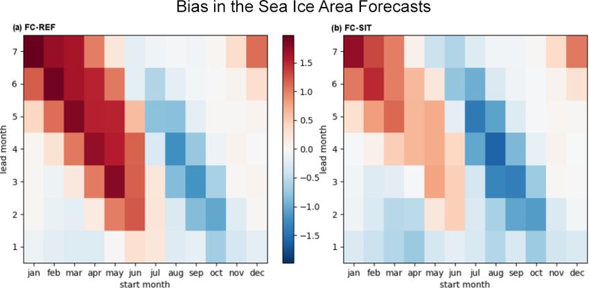
328                        B. Balan-Sarojini et al.: Impact of winter sea ice thickness observations on seasonal forecasts

2.2     Methods                                                 ever, we note that only the ocean reanalysis ORAS5 actually
                                                                makes use of the albedo computed by LIM2 (which is too
2.2.1    Ocean–sea-ice reanalysis experiments                   high in summer), while the atmospheric reanalyses used for
                                                                verification and the forecasting system use the same clima-
In order to assess the impact of new sea ice thickness obser-   tological albedo (based on SHEBA campaign observations;
vations on the assimilation, we carry out two ORAs as shown     Beesley et al., 2000). Moreover, a recent comparison study
in Table 1. They are (1) a reference experiment with SIC as-    (Pohl et al., 2020) shows that, overall, the broadband albedo
similation (ORA-REF) and (2) an experiment with SIC as-         over Arctic sea ice derived from MERIS observations is com-
similation and sea ice thickness constraint (ORA-SIT). Ex-      parable to that in the ERA5 atmospheric reanalysis in terms
periments ORA-REF and ORA-SIT are run for the time pe-          of the seasonal cycle on large spatial scales. The forecast
riod January 2011 to December 2016, because these are the       albedo over ice is comparable to that in ERA5 and ERA-
full years for which CS2SMOS observations were available        Interim atmospheric reanalyses. LIM2 has a time step of 1 h
at the time of experimentation. Note that ORA-REF is a con-     and is coupled to the ocean at every time step.
tinuation of a longer experiment which started in 2005, and        As for ORAS5, both experiments here use the variational
ORA-SIT starts from ORA-REF on 1 January 2011.                  data assimilation using NEMOVAR in a 3D-Var FGAT (first
   Our reanalysis experiments are forced by near-surface air    guess at appropriate time) configuration as described in Mo-
temperature, humidity, and winds as well as surface radia-      gensen et al. (2012). The length of the assimilation window
tive fluxes from the atmospheric reanalysis ERA-Interim         is 10 d in our experiments. Assimilated observations com-
(ERA-I) (Dee et al., 2011) until 2015 and from the ECMWF        prise temperature and salinity profiles, altimeter-derived sea
operational analysis from 2015 to 2016. We use the same         level anomalies and sea ice concentration. Sea surface tem-
set-up of NEMOVAR (variational data assimilation system         perature is constrained to observations by a strong relaxation.
for NEMO (Nucleus for European Modelling of the Ocean)          A global freshwater correction is added to reproduce the ob-
ocean model) used in ORAS5 (Zuo et al., 2019) – in par-         served global-mean sea level change. The assimilation of the
ticular, almost the same observations are assimilated. The      SIC is done separately from the ocean variables and is de-
only differences are the following: (a) a coarser model res-    scribed in Tietsche et al. (2015) and Zuo et al. (2017).
olution as described below, (b) different assimilated SIC ob-      In addition to the observations assimilated via
servations compared to the current operational one and (c) a    NEMOVAR, the SIT in experiment ORA-SIT is con-
longer assimilation window of 10 d instead of 5 d.              strained to the CS2SMOS via a linear nudging technique
   The ocean general circulation model used in these experi-    (Tietsche et al., 2013; Tang et al., 2013). The relationship
ments is NEMO version 3.4 (Madec, 2008) with a horizontal       between the modelled and observed sea ice thickness in a
resolution of approximately 1◦ and 42 vertical layers. The      grid point is described by the following equation:
grid is tripolar, with the poles over Northern Canada, Cen-
tral Asia and Antarctica enabling higher resolution across          n       1t
                                                                            m      m     o
                                                                SIT = SIT −    (SIT − SIT ) ,                                (1)
the Arctic than at the Equator. The first model layer is 10 m               τ
thick, and the upper 25 levels represent approximately the
top 880 m. Both the horizontal and vertical resolution in our   where SITn is the nudged thickness, SITm is the modelled
set-up is lower than that of the current operational system,    floe thickness, SITo is the observed floe thickness, 1t is the
which has a horizontal resolution of approximately 0.25◦ and    sea ice model time step of 1 h, and τ is the nudging coef-
75 vertical levels. The time step is 1 h.                       ficient corresponding to a relaxation timescale of 10 d. The
   The prognostic thermodynamic–dynamic sea ice model           choice of a 10 d relaxation timescale makes sense as a first
used is LIM2 (Louvain-la-Neuve Sea Ice Model) in its orig-      trial, since it is consistent with the length of the assimilation
inal version (Fichefet and Maqueda, 1997). The vertical         window. To facilitate the nudging, the CS2SMOS weekly
growth and decay of ice due to thermodynamic processes is       observations in EASE2 grid have been interpolated to daily
modelled according to the three-layer (one layer for snow and   gridded fields in the ORCA 1◦ grid. The weekly to daily in-
two layers for ice) Semtner scheme (Semtner, 1976). The ice     terpolation is done by appropriately weighting two adjacent
velocity is calculated from a momentum balance considering      weekly-mean fields. We have also tested the sensitivity to
sea ice as a two-dimensional continuum in dynamical inter-      different nudging strengths by running variants of ORA-SIT
action with the atmosphere and ocean. Internal stress within    with a relaxation timescale of 20, 30 and 60 d. By construc-
the ice for different states of deformation is computed fol-    tion, as the relaxation timescale increases from 10 to 60 d,
lowing the viscous–plastic (VP) rheology proposed by Hi-        SIT is less constrained to CS2SMOS. In this study, we only
bler (1979). LIM2 has a single sea ice category to represent    use the experiment with the strongest constraint (10 d relax-
sub-grid-scale ice thickness distribution, and open water ar-   ation time) for initializing the ensemble reforecasts, because
eas like leads and polynyas are represented using ice concen-   this timescale fits with the length of the assimilation window,
tration. Melt ponds are not modelled, which could affect the    and we aimed for a strong observational constraint in order
accurate representation of surface albedo over sea ice. How-    to obtain a strong forecast impact.

The Cryosphere, 15, 325–344, 2021                                                    https://doi.org/10.5194/tc-15-325-2021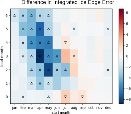
B. Balan-Sarojini et al.: Impact of winter sea ice thickness observations on seasonal forecasts                                      329

Table 1. Specifications of the ocean–sea-ice assimilation experiments.

                Experiment name      SIC constraint    SIT constraint    Time period    Description
                ORA-REF              Yes               No                2011–2016      SIC assimilation
                ORA-SIT              Yes               Yes               2011–2016      SIC assimilation and SIT nudging

2.2.2   Coupled reforecast experiments                                   skill of seasonal forecast of sea ice area, sea ice edge, sea ice
                                                                         volume and 2 m temperature. When possible, we use the ob-
In order to assess the impact of CS2SMOS sea ice thick-                  servational datasets for verification. However, as mentioned
ness initialization on sea ice forecasts, we performed two sets          above, sea ice thickness and volume (SIV) cannot be ver-
of twin coupled ocean–sea-ice–atmosphere reforecast exper-               ified properly for the months of April–October, due to the
iments as shown in Table 2, which only differ in the ocean–              lack of sea ice thickness observations. In those cases, we will
sea-ice initial conditions provided by the data assimilation             describe the impact in terms of differences between experi-
experiments shown in Table 1. The reference reforecast (FC-              ments. We use the term pan-Arctic to refer to all regions of
REF) is initialized by ORA-REF, and reforecast experiment                the Northern Hemisphere that are potentially covered by sea
FC-SIT is initialized by ORA-SIT. Comparison of results                  ice.
from these two sets of reforecasts allows quantifying the im-
pact of SIT information on the seasonal forecasts.
                                                                         3.1   Impact of sea ice thickness initialization on the sea
   The reforecast experiments are carried out using a version
                                                                               ice reanalysis
of the ECMWF coupled seasonal forecasting system. The
coupled model consists of the same ocean and sea ice model
(NEMO3.4/LIM2) used for our reanalysis experiments and is                Figure 1 shows the SIT bias with respect to the CS2SMOS
coupled to the ECMWF atmospheric model, Integrated Fore-                 observations for ORA-REF (Fig. 1a, c) and ORA-SIT
cast System (IFS) version 43r3. It is run with a horizontal              (Fig. 1b, d) for March (Fig. 1a, b) and November (Fig. 1c,
resolution of 36 km, corresponding to a cubic octahedral re-             d). The ORA-REF suffers from large ice thickness bias of
duced Gaussian grid at truncation TCo319 and 91 vertical                 up to 1.4 m. The predominant bias pattern is an underes-
levels (SEAS5 is run with IFS cycle 43r1 at the same atmo-               timation of ice thickness by more than 1 m in the central
spheric resolution but with 0.25◦ horizontal resolution and              Arctic and an overestimation in the Beaufort Gyre and the
75 vertical levels in the ocean). The coupled model also in-             Canadian Archipelago of the order of 1 m. This pattern is
cludes the land surface model HTESSEL (Hydrology Tiled                   present for all the months when CS2SMOS is available. In
ECMWF Scheme for Surface Exchanges over Land) and the                    March, widespread overestimation in the coastal Arctic seas
ocean surface wave model WAM. The coupling of the at-                    is also present. These biases are much reduced or absent in
mosphere and ocean is done using a Gaussian interpolation                ORA-SIT. Most of the large-scale pattern of underestimation
method, and the coupling frequency is 1 h. For more details              and overestimation of sea ice in ORA-REF is not present
on SEAS5, see Stockdale et al. (2018) and Johnson et al.                 in ORA-SIT in March. However, a slight underestimation
(2019).                                                                  over the central Arctic and an overestimation over the Cana-
   Both reforecasts are started on the first of each month of            dian Archipelago still remain in November. This is caused
each year from 2011 to 2016, resulting in 72 forecast start              by the lack of SIT observations during the months preceding
dates overall. Note that out of all months of each year in the           November. In contrast, the estimation of the March condi-
2011–2016 period only winter (December–April) months are                 tions benefits from the availability of SIT information in the
directly constrained by November–March observations as the               preceding winter. We note that the bias in ORA-SIT over the
CS2SMOS data are only available for those 5 full months.                 Laptev, East Siberian and Chukchi seas is very small, about
The initial conditions for the remaining 7 start months (May–            0.1 to 0.05 m of magnitude (below the contour interval).
November) of each year are indirectly affected by the thick-                Figure 2 shows the difference in SIT between ORA-SIT
ness constraint applied earlier in the ice growth season in the          and ORA-REF for March, July, September and November.
reanalysis. The forecast initialized from each start date has            The difference patterns between ORA-SIT and ORA-REF
25 ensemble members for both sets of reforecasts.                        are quite consistent for all the months, characterized by a
                                                                         thickening of the thick ice over the central Arctic and north
                                                                         of Greenland, as well as a thinning of the thin-ice area over
3   Results                                                              the Beaufort and Siberian seas, thus enhancing the spatial
                                                                         gradients in the sea ice thickness distribution. The largest
Here we first assess the impact of sea ice thickness obser-              impact occurs in March, probably because at this month the
vations on the estimation of sea ice properties in the ORA               SIT observations have been assimilated during the preceding
initial conditions, and then we evaluate the impact on the               5 months. The impact of SIT winter information lasts well

https://doi.org/10.5194/tc-15-325-2021                                                            The Cryosphere, 15, 325–344, 2021
330 B. Balan-Sarojini et al.: Impact of winter sea ice thickness observations on seasonal forecasts
Table 2. Overview of the reforecast experiments. For each of the start years, forecasts are started on the first of every calendar month.
Experiment name Start years Lead month Ensemble size Initial condition Description
FC-REF 2011–2016 7 25 ORA-REF SIC initialization
FC-SIT 2011–2016 7 25 ORA-SIT SIC and SIT initialization
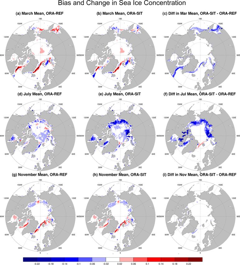
Figure 1. Bias in monthly-mean (2011–2016) sea ice thickness (m) in experiment (a) ORA-REF and (b) ORA-SIT for March (a, b) and
November (c, d). The reference is CS2SMOS observations. ORA-REF is the ocean–sea-ice assimilation experiment with no sea ice thickness
constraint. ORA-SIT is the assimilation experiment with a thickness relaxation timescale of 10 d.
The Cryosphere, 15, 325–344, 2021 https://doi.org/10.5194/tc-15-325-2021B. Balan-Sarojini et al.: Impact of winter sea ice thickness observations on seasonal forecasts 331 Figure 2. Difference in monthly-mean (2011–2016) sea ice thickness (m) between experiments ORA-SIT and ORA-REF for (a) March and (b) July and for (c) September and (d) November months. into the summer months, with a slight clockwise displace- In March, the month of sea ice maximum, ORA-REF shows ment of the thinning and a reduction of the thickening, which mostly an overestimation of SIC all around the sea ice edge, by September has roughly halved. The shift in the thinning over the Davis Strait, northeast of Greenland, the Bering Sea pattern is consistent with the mean climatological transpolar and the Okhotsk Sea. In ORA-SIT this bias is uniformly re- Arctic drift pattern and is thus likely a consequence of the duced by up to 10 % . In November (Fig. 3g, h and i), when mean advection. The impact during March and November is the sea ice edge is expanding with newly frozen ice, ORA- consistent with a reduction of the bias in ORA-REF (Fig. 1a REF has similar SIC overestimation biases over the ice edge, and c). Since basin-scale SIT observations are not available but this time the SIT constraint has very little impact on SIC for the end of the melt season, biases are unknown. biases. This is because of no SIT nudging happening in the The thickness constraint also affects the biases in SIC. Fig- preceding months. Also, the very small changes in SIC bias ure 3 shows the SIC bias with respect to OSI-401-b SIC as between ORA-REF and ORA-SIT over the Chukchi and East well as the SIC difference between ORA-REF and ORA-SIT. Siberian Sea regions of negligible ice thickness bias in ORA- https://doi.org/10.5194/tc-15-325-2021 The Cryosphere, 15, 325–344, 2021
332                           B. Balan-Sarojini et al.: Impact of winter sea ice thickness observations on seasonal forecasts

Figure 3. Bias in monthly-mean (2011–2016) sea ice concentration with respect to OSI-401-b observations for ORA-REF (a, d, g), ORA-
SIT (b, e, h), and the difference between ORA-SIT and ORA-REF for panels (c), (f) and (i). Panels (a), (b) and (c) are for March; panels (d),
(e) and (f) are for July; and panels (g), (h) and (i) are for November.

SIT (Fig. 1d) are suggestive of fast growth processes in the             servations exerts to compensate for errors in the sea ice state.
forward model, which is faster than the timescales intrinsic             Figure 4 shows the mean annual cycle of the area-averaged
to the SIC assimilation. The ORA-REF biases in July are                  assimilation increments in ORA-REF (blue) and ORA-SIT
characterized by a weak underestimation of SIC. Notably,                 (green). In both experiments, the assimilation increments ex-
in ORA-SIT there is an increase in the negative SIC bias of              hibit a clear seasonal cycle, with large positive increments
more than 10 % over the Pacific and Siberian Arctic sectors              from May to October, indicative of strong underestimation
towards the end of melt season, with July and August (not                of SIC in the forward model, and weak negative increments
shown) months being the most affected.                                   from December to March. The differences in SIC increments
   To gain some insight into the degradation of the July SIC             over the Arctic between the two experiments peak during
bias in ORA-SIT, we look at the mean annual cycle of the                 July, with ORA-SIT increments about 9 % per month higher
SIC assimilation increments. The assimilation increments are             than in ORA-REF. The results in this figure indicate that
indicative of the corrections that the assimilation of SIC ob-           (1) both ORAs melt sea ice too fast during the summer

The Cryosphere, 15, 325–344, 2021                                                              https://doi.org/10.5194/tc-15-325-2021
B. Balan-Sarojini et al.: Impact of winter sea ice thickness observations on seasonal forecasts                                 333

                                                                    ases shown in FC-REF are quite similar to those in SEAS5
                                                                    (not shown), which are discussed in more detail in Stockdale
                                                                    et al. (2018). The positive biases in the melt season forecasts
                                                                    are considerably reduced with the SIT initialization in FC-
                                                                    SIT started in January to June, and the negative biases in the
                                                                    forecasts are worsened in FC-SIT started in July to October
                                                                    (Fig. 5b). The forecasts for winter months remain unbiased
                                                                    in FC-SIT. Note that the bias regimes in the forecasts are very
                                                                    different from the bias regimes in the reanalysis (Sect. 3.1),
                                                                    which tends to have too much ice in winter and too little ice
                                                                    in summer.
Figure 4. Annual cycle of the mean of the SIC increments in ORA-       The impact of thickness initialization has not only im-
SIT (green) and ORA-REF (blue), averaged over the area north of     proved the biases in summer SIC forecasts, but it has also
70◦ N during 2011–2016. The grey shading shows months (January      improved the sea ice edge forecasts as measured by the in-
to March and November to December) with CS2SMOS SIT nudg-           tegrated ice edge error (IIEE) (Fig. 6). Seasonal forecasts of
ing.                                                                ice edge are in great demand for exploring economically vi-
                                                                    able Arctic shipping routes. IIEE is one of the recent user-
                                                                    relevant sea ice metrics on ice extent or ice edge (Goessling
months, as shown by negative SIC biases in the marginal             et al., 2016; Bunzel et al., 2017). Since it can be decomposed
seas of the Arctic Ocean where thin sea ice resides during          into over- and under-prediction, it is more useful than the tra-
the summer months (Fig. 3d and e); and (2) the SIT assim-           ditional basin-wide sea ice extent error.
ilation exacerbates the summer SIC biases in ORA-SIT (as               For simplicity, we assess ice edge forecasts by using the
seen in e.g. Fig. 3e) due to corrected but thinner sea ice at the   deterministic IIEE metric calculated from the ice edge of the
beginning of the melt season in almost all marginal seas of         ensemble mean SIC forecasts. We have also tested proba-
the Arctic Ocean (Fig. 2a).                                         bilistic metrics like the Spatial Probability Score suggested
   From January to May and from November to December,               by Goessling and Jung (2018) and found that they give very
on average less ice is being taken away by the increments           similar results.
in the ORA-SIT (green) analysis than that in ORA-REF                   IIEE for all lead months and start months verified against
(Fig. 4). These results clearly show the long-lasting effect of     OSI-401-b suggests reduced error in sea ice edge (blue
the SIT information: the SIT constraint was only applied dur-       colours) in FC-SIT overall. The most striking feature is the
ing the growth season from November to March (grey shad-            significant improvement in summer forecast error for lead
ing), but its impact, whether positive or negative, is evident      months 2–7 in FC-SIT compared to FC-REF. The main con-
in sea ice concentration throughout the melting season even         tribution to the error reduction of up to 30 % in summer fore-
in the presence of SIC assimilation.                                casts comes from the reduction of the model bias, leading
                                                                    to consistent over-prediction (not shown). For the traditional
3.2   Impact of ice thickness initialization on sea ice             September sea ice extent forecast starting in April, an im-
      forecasts                                                     provement of 28 % is found. Forecast verification in October
                                                                    and November from July and August starts shows a slight
Figure 5a gives an overview of bias in the sea ice area in          degradation caused by under-prediction (not shown). This
the FC-REF reforecast with respect to the ORAS5 reanaly-            could again be due to the indirect effect of a thinner start-
sis as a function of forecast start and lead months. ORAS5          ing point in FC-SIT (Fig. 2b) and a lower, degraded SIC in
is preferred to OSI SAF for the verification of integrated sea      the ORA-SIT reanalysis (Fig. 3e), combined with the already
ice area because of its complete spatial coverage. The fig-         existing slow-refreeze nature of the model.
ure shows the forecast bias for different forecast lead times          Figures 5 and 6 point out that the impact of ice thick-
(y axis) as a function of forecast starting month (x axis).         ness initialization on the forecast bias and errors is strongly
Errors at lead month 1 are generally small throughout the           dependent on season and lead time. Most seasons and lead
year. However, for longer lead times, there is a strong over-       times are improved, but some are, perhaps inevitably, deteri-
prediction of sea ice area in summer months and a moder-            orated. To measure the overall impact on forecast error and
ate under-prediction of autumn sea ice conditions, consistent       make a statement about potential skill improvements that are
with a melting that is too slow and refreeze that is slow re-       to be expected for operational forecasts, we aggregate FC-
spectively. The forecast biases are generally small in winter       SIT and FC-REF for all start months from January 2011 to
months.                                                             December 2016 and compute the area-integrated mean abso-
   These three bias regimes in general – small bias in win-         lute forecast error (MAE) of sea ice concentration for each
ter, positive bias in summer and negative bias in autumn –          lead month. In order to obtain the bias-corrected forecast
seem to be mostly independent of start months. These bi-            value, for each combination of grid cell, start date and fore-

https://doi.org/10.5194/tc-15-325-2021                                                      The Cryosphere, 15, 325–344, 2021
334 B. Balan-Sarojini et al.: Impact of winter sea ice thickness observations on seasonal forecasts
Figure 5. Bias in the forecast of pan-Arctic sea ice area (×106 km2 ) with respect to ORAS5 as a function of start and lead month for 2011–
2016 (a) in the reference reforecast FC-REF and (b) in the SIT-initialized reforecast FC-SIT. Red colour denotes over-prediction of sea ice
area, and blue colour denotes under-prediction.
ification data valid for the same calendar month but differ-
ent years from the range of target months considered (Jan-
uary 2011 to June 2017).
Averaged over all start dates and grid points, Fig. 7 shows
that the MAE of sea ice area is substantially improved in FC-
SIT. When no bias correction is applied prior to computing
the MAE (Fig. 7a), FC-SIT forecasts are significantly better
in each lead month, with a maximum error reduction of about
10 %.
However, skill assessments of seasonal forecasts are con-
ventionally made after a forecast calibration where the im-
pact of the forecast bias is removed. By this measure, a re-
duction of forecast bias does not by itself count as an im-
provement. As Fig. 7b shows, removing the respective bias
of FC-SIT and FC-REF prior to computing the MAE results
in a smaller error reduction: errors in FC-SIT are signifi-
cantly lower only in lead months 2–5 by up to 5 %. Figure 7
demonstrates that, although the thickness initialization pre-
Figure 6. Difference in integrated ice edge error in 105 km2 be- dominantly reduces the bias, it also leads to an improvement
tween FC-SIT and FC-REF reforecasts for 2011–2016 with respect in the skill of sea ice area forecasts that is relevant for opera-
to OSI-401-b observations. Blue colour denotes reduced error in tional forecasting systems.
sea ice edge in FC-SIT and red colour denotes increased error in The importance of forecast biases is illustrated by bench-
FC-SIT. Black triangles represent statistical significance at the 5 % marking the errors of the dynamical forecasting system
level according to the sign test (DelSole and Tippett, 2016). against a simple statistical reference forecast: Figure 7 also
shows the errors of a climatological reference forecast (FC-
clim). Without bias correction, errors of both FC-REF and
cast lead time, we compute the mean forecast error over all FC-SIT are larger than those from FC-clim already after
forecasts and then subtract it from the raw forecast value. 1 month, while after bias correction both FC-REF and FC-
Comparison against a climatological benchmark forecast is SIT have lower errors than FC-clim for all lead months.
a very useful background information for evaluating the pre- Finally, we analyse the impact of SIT initialization on fore-
dictive skill of ensemble forecasting systems (e.g. Zampieri casts of pan-Arctic sea ice volume. Though an integrated
et al., 2018). The climatological reference forecast for a quantity like pan-Arctic sea ice volume is a result of many
given target month and year is constructed by using the ver- dynamic and thermodynamic sea ice processes and lacks re-
The Cryosphere, 15, 325–344, 2021 https://doi.org/10.5194/tc-15-325-2021B. Balan-Sarojini et al.: Impact of winter sea ice thickness observations on seasonal forecasts 335
Figure 7. Spatially integrated SIC mean absolute error over lead month for all FC-REF and FC-SIT forecasts (72 forecasts each first of the
month from January 2011 to December 2016) with respect to OSI-401-b observations. Panel (a) shows the error in 106 km2 without bias
correction and panel (b) the error in 105 km2 after bias correction. Lead months for which the reduction of forecast error in FC-SIT passes a
statistical significance test at the 5 % level (DelSole and Tippett, 2016) are marked by filled circles, and insignificant changes are marked by
crosses. The error of a simple climatological reference forecast is also shown as FC-clim.
(top) and August (bottom). The forecast climate is computed
by averaging the reforecast starting at a given calendar month
for the years 2011–2015. Seven month forecasts started in
August lead to February of the following year. Since the
ORAs are not available in January and February 2017, the
year 2016 is not accounted for in this figure. For reference,
the sea ice volume estimates of ORA-REF and ORA-SIT re-
analyses are also shown. It is remarkable that the shape of
the seasonal cycle is largely preserved between FC-REF and
FC-SIT, maintaining the initial offset during the whole fore-
cast range. The figure clearly shows that FC-SIT starts from
a thinner ice state than FC-REF in both initial months.
The May starts show large differences between the fore-
casts and the ORAs: both FC-SIT and FC-REF show a slower
SIV decrease (lower melt rate) than the ORAs from June to
September and also a slower refreeze during October and
November. The explanation for the different behaviour of the
ORAs and the forecasts is that the ORAs are constrained by
the same SIC (but not the same SIT) information in summer,
which leads to the convergence of the sea ice state in the
Figure 8. Time series of ensemble mean sea ice volume (units
are 104 km3 ) forecasts averaged over 2011–2015 for the May start
ORAs during that time of the year (also seen in Fig. 4). In
date (a) and August start date (b) in reference reforecast (FC-REF, the coupled forecasts, there is no similar constraint and they
dashed blue line) and reforecast with thickness initialization (FC- tend to converge slower than the ORAs. The melt rates of the
SIT, dashed green line) compared to their own reanalyses, ORA- ORAs here are consistent with those in ORAS5 (see Uotila
REF (solid blue line), and ORA-SIT (solid green line). et al., 2019, or Mayer et al., 2019). Compared to the May
starts, differences between FC-SIT and FC-REF are smaller
in the August starts, and so is their agreement with the ORAs.
gional details, it is a key indicator for understanding the Arc- Again, the FC-SIT shows smaller values than FC-REF from
tic energy cycle, an important process that needs to be real- the beginning, and both forecast sets exhibit a parallel SIV
istically represented in reanalyses and seasonal forecasts. It evolution. The shape of the seasonal cycle in the forecasts
is useful to compare the contrasting SIV seasonal cycles in is different from the ORAs; the forecasts initialized in Au-
coupled and uncoupled mode and with/without SIT observa- gust show a slower refreeze during October than the ORAs.
tional constraint in the initialization, since this helps to iden- However, after October, the SIV increases faster in the fore-
tify the origin of errors in the systems in the specific opera- casts than in ORA-SIT, and it continues increasing more or
tional set-up. Figure 8 shows the sea ice volume forecast cli- less at the same rate until the end of January in the forecasts,
mate at different lead months for the forecasts starting in May
https://doi.org/10.5194/tc-15-325-2021 The Cryosphere, 15, 325–344, 2021336 B. Balan-Sarojini et al.: Impact of winter sea ice thickness observations on seasonal forecasts
MET from lead month 1 data from each start date. Assimila-
tion increments of SIC proportionally affect SIV in the ORAs
(Tietsche et al., 2013, 2015). The resulting MET increments
are shown for both ORA-REF and ORA-SIT as well. We
note that the MET annual cycle of ORA-REF is very sim-
ilar to that of ORAS5 (not shown) and that the average of
the MET annual cycle in the ORAs is close to zero (in fact
about +0.3 W m−2 (Mayer et al., 2016, 2019), in agreement
with the long-term sea ice melt), while it is −4.8 W m−2 in
FC-REF.
Figure 9 clearly shows that ORA-REF exhibits the most
pronounced annual cycle of MET, with strongest melting in
summer and strongest freezing in winter. Earlier studies have
shown that the MET annual cycle is exaggerated in ORAS5
(Uotila et al., 2019; Mayer et al., 2019) and hence also in
Figure 9. Mean annual cycle of MET over the ocean area north of ORA-REF. ORA-SIT has a damped MET annual cycle, as
70◦ N in ORA-REF, ORA-SIT, FC-REF (lead month 1) and FC-SIT the thickness constraint during winter prevents overly strong
(lead month 1). MET increments for ORA-REF and ORA-SIT are SIV accumulation. Lower SIV at the end of winter conse-
shown as well. quently leads to weaker melting in summer. However, sum-
mer melt in ORA-SIT is likely still too strong, as this experi-
while in ORA-SIT (solid green line) the freezing rate slows ment features a negative SIC bias in summer despite realistic
down after November. As a result by the end of January the SIT and SIC earlier in the year, when CS2SMOS data are
forecast SIV is higher than in ORA-SIT. ORA-REF without available (see Fig. 3e).
the thickness constraint has the highest SIV in the ice growth Both FC-REF and FC-SIT agree very well with each other
season. In the next section we examine the discrepancies in and exhibit a much weaker MET annual cycle than the ORAs
SIV changes between ORAs and FCs in more detail. (Fig. 9). The difference between the forecasts and the ORAs
in May and June melting cannot be explained by the MET
3.3 Linking sea ice analysis and forecast errors to the increments (neutral impact at that time), which points to dif-
Arctic surface energy budget ferences in energy fluxes into the sea ice as a cause.
We therefore compare the mean annual cycle of surface
In order to investigate the physical causes of sea ice errors in net radiation (RadS ) over the ocean north of 70◦ N. Fig-
the ORAs and forecasts, the Arctic surface energy budget is ure 10a shows the 2011–2015 annual cycle of RadS from FC-
considered. We estimate melt energy tendency (MET), which REF, FC-SIT, ERA-I, ERA5, and the satellite-based product
is the energy used to melt sea ice and energy released in the Clouds and Earth’s Radiant System–Energy-Balanced and
process of freezing and is proportional to SIV changes. It is Filled surface edition 4.0 (CERES-EBAF; Kato et al., 2018),
defined as in Mayer et al. (2019): which we use as reference.
We consider RadS from ERA-I a good proxy for RadS seen
∂SIT
MET = Lf ρ , (2) by the ORAs for two reasons: (1) ORAs use ERA-I forcing
∂t during most of the study period, and (2) ORAs do not output
where Lf denotes latent heat of fusion (−0.3337 × the RadS term, although it is not exactly identical for exam-
106 J kg−1 ), ρ represents sea ice density (assumed constant ple due to different albedo in the ORAs. ERA-I exhibits a
at 928 kg m−3 ), and SIT is the grid-point-averaged sea ice positive RadS bias in summer, peaking in June at 15 W m−2 ,
thickness. Thickness changes are computed as exact monthly while FC-REF and FC-SIT agree quite well with CERES-
differences. MET can also change dynamically through lat- EBAF, especially in May and June, when MET discrepan-
eral ice transports, but here we average over the ocean area cies with the ORAs are large (Fig. 9). Thus the RadS bias of
north of 70◦ N, which should be a sufficiently large area to ERA-I can explain a large fraction of the overly strong MET
average out any dynamical effects and should mainly leave in the ORAs during May and June, as well as the discrepancy
thermodynamic effects as the drivers of MET. Figure 9 shows between the ORAs and the forecasts.
the MET mean annual cycle (2011–2015) north of 70◦ N for The mean deviation of RadS from CERES-EBAF
ORA-REF, ORA-SIT, FC-REF and FC-SIT. In order to iso- (Fig. 10b) clearly indicates that forecasts are closer to the ob-
late the changes in MET when switching from forced ORA servational product than the atmospheric reanalyses in May
mode to coupled forecast mode and to avoid seeing mainly and June. This positive RadS bias of ERA-I should be consid-
the effect of feedbacks arising from the model sea ice state ered alongside the results by Hogan et al. (2017), who found
drifting away from the analysed state (most notably the ice– a negative bias in downwelling shortwave radiation in ERA-
albedo feedback), we compile the annual cycle of forecasted I due to excessive low-level clouds. Our results can be ex-
The Cryosphere, 15, 325–344, 2021 https://doi.org/10.5194/tc-15-325-2021B. Balan-Sarojini et al.: Impact of winter sea ice thickness observations on seasonal forecasts 337
to FC-REF. The bias reduction can be attributed to the im-
proved initial conditions in FC-SIT, but the fact that the sea
ice area bias remains positive from July onward indicates that
MET in the forecasts is too low in summer. Figure 10b sug-
gests that RadS is too low in the forecasts in July and August,
which probably contributes to the positive sea ice area bias
remaining in FC-SIT (Fig. 5b).
The October MET (Fig. 9) indicates stronger refreeze in
the ORAs (lower MET values) compared to the forecasts.
This is consistent with negative MET increments present in
the ORAs, which act to speed up refreeze in the reanalyses
(see Fig. 9). The less negative MET values of the forecasts
in October are consistent with the freezing that is too weak
and consequent underestimation of sea ice in autumn in the
August starts.
Area-averaged net radiation of all considered products
agrees well with CERES-EBAF in October (see Fig. 10), and
also difference maps show only a weakly positive RadS bias
of the reanalyses and forecasts compared to CERES-EBAF
(not shown). Hence, errors in other physical terms such as
ocean–ice fluxes must play an important role in autumn, but
more detailed investigations are beyond the scope of this pa-
per.
3.4 Impact of ice thickness initialization on forecasts of
atmospheric variables
To discuss the impact of the sea ice thickness constraint on
the atmosphere, we first assess the differences in the forecast
means (or biases) between FC-SIT and FC-REF. Figure 11a
shows the bias in 2 m temperature (T2m) (averaged over
50–90◦ N) in FC-REF as a function of start dates and lead
Figure 10. (a) Mean annual cycle of surface net radiation, RadS months. When verified against ERA5, significant cold biases
(W m−2 ), over the ocean area north of 70◦ N from ERA-I, ERA5,
are present in forecasts for most of the start months and lead
FC-REF (lead month 1), FC-SIT (lead month 1) and CERES-EBAF
months except for non-significant warm biases in November
and (b) mean deviation of RadS from CERES-EBAF for FC-REF,
FC-SIT, ERA-I and ERA5. forecasts started in August, September and October months.
We note that using atmospheric or ocean reanalysis with-
out realistic representation of snow over sea ice, and sea ice
thickness, for the verification of pan-Arctic surface tempera-
plained by the positive bias in downwelling longwave radia- ture can be misleading, since there is large uncertainty asso-
tion in ERA-I outweighing the shortwave flux bias. Figure 10 ciated with these products (Batrak and Müller, 2019). Verify-
also shows results for ERA5, which is closer to CERES- ing against observations is not easy, since due to the scarcity
EBAF than ERA-I, which indicates a reduced cloud bias of observational campaigns over sea ice, the verification will
in this more-recent atmospheric reanalysis and gives rise to have large representativeness error and hence is not suitable
the expectation of improved MET in future ocean reanalyses for seasonal forecasts verification. Mean differences in T2m
forced by this product. We also note that the mean differ- (Fig. 11b) are generally positive with very few and non-
ence in sensible heat fluxes in ERA-Interim and the forecasts significant exceptions, which is expected from the generally
and differences over sea ice were uniformly small (gener- reduced sea ice cover in FC-SIT. The strongest warming with
ally < 2 W m−2 in summer; not shown), confirming that dif- area averages of 0.5 K can be found during autumn for fore-
ferences in this field cannot explain the found differences in casts started between March and September. February and
MET. March start dates show a moderate but significant warming
Additional information on the realism of summer MET in at short lead times, but otherwise changes are relatively small
the forecasts can be obtained from the sea ice area forecast for October to February start dates. Also, changes in summer
bias of FC-SIT, as displayed in Fig. 5b. It shows that FC-SIT temperatures are small compared to those in autumn. Inspec-
May starts exhibit a strongly reduced positive bias compared tion of temperature difference patterns between FC-SIT and
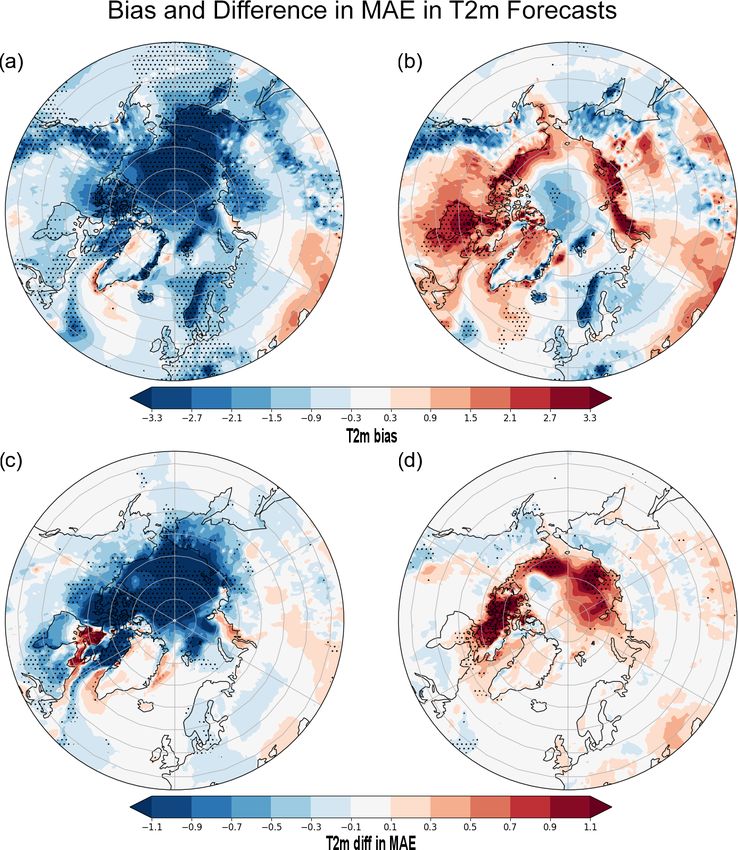
https://doi.org/10.5194/tc-15-325-2021 The Cryosphere, 15, 325–344, 2021338 B. Balan-Sarojini et al.: Impact of winter sea ice thickness observations on seasonal forecasts Figure 11. Mean forecast differences between FC-SIT and FC-REF 2011–2016: (a) bias in mean 2 m temperature (in K) north of 50◦ N with respect to ERA5, as a function of start dates and lead months, in FC-REF; panel (b) is similar to panel (a) but with a difference in mean 2 m temperature (in K) between FC-SIT and FC-REF. Triangles denote significant changes according to the sign test as recommended by DelSole and Tippett (2016) at the 5 % level. Mean forecast difference (FC-SIT – FC-REF) for SON aggregated from May, June, July and August start dates of (c) 2 m temperature and (d) mean sea level pressure. Dots indicate areas of significant changes on the 95 % level according to the Kolmogorov–Smirnov test. FC-REF indicates that differences in summer are confined to to North America and Eurasia. Solar radiation in the Arc- areas around the sea ice edge (not shown), while changes in tic is very weak for SON. Hence, the warming in FC-SIT autumn are more widespread (see Fig. 11c). The warming must stem from enhanced fluxes of heat from the ocean to pattern in autumn appears as a diagonal feature in Fig. 11b, the atmosphere, with a possible positive feedback from in- which suggests that changes depend more on season than on creased atmospheric water vapour. The fluxes are enhanced forecast lead time. Therefore, to gain more insight into the in FC-SIT due to larger areas of open waters and increased spatial structure of the changes, Fig. 11c and d show fore- SSTs, both a result of reduced sea ice concentration. Further- cast differences in 2 m temperature and mean sea level pres- more, we find warming over the northwest Atlantic, which sure in SON, respectively. To find robust changes, the differ- is related to the warmer SSTs present already in the ini- ences are aggregated from forecasts started between May and tial conditions from ORA-SIT (not shown). Another area of August, yielding samples of 600 forecasts. Moreover, aggre- significant warming in FC-SIT relative to FC-REF can be gation along the diagonal maximizes the signal (compare to seen over Eastern Europe and western Russia. This warm- Fig. 11b). ing seems consistent with patterns of mean sea level pres- Widespread temperature differences > 1 K can be seen sure differences shown in Fig. 11d. They show lower pres- over the Arctic Ocean and the Canadian Archipelago in sure in FC-SIT over Scandinavia and higher pressure over SON (Fig. 11c), but significant warming spreads also south central Russia, which together suggest more southerly winds The Cryosphere, 15, 325–344, 2021 https://doi.org/10.5194/tc-15-325-2021
B. Balan-Sarojini et al.: Impact of winter sea ice thickness observations on seasonal forecasts                                  339

in the region of warmer temperatures. Furthermore, mean             4   Summary and concluding remarks
sea level pressure changes indicate lower pressure over the
Arctic Ocean and the Canadian Archipelago, i.e. in areas            In this paper we use 6 years of Arctic-wide sea ice thickness
of maximum warming. In addition, there are positive pres-           observations of January, February, March, November and
sure differences southeast of Greenland. Altogether, the pat-       December months during 2011 to 2016 to constrain the mod-
terns in sea level pressure difference resemble a wave-like         elled sea ice thickness and study the impact on the ocean–
response, but it should be kept in mind that only some parts        sea-ice reanalysis. Coupled forecasts of the ocean–sea-ice–
of these changes are statistically significant. Nevertheless,       wave–land–atmosphere are initialized using these data as-
we note that qualitatively similar and significant changes are      similation experiments, and the forecast skill of pan-Arctic
also found in 500 hPa geopotential forecasts for SON (not           sea ice for lead times up to 7 months is investigated. To our
shown), suggesting that the features seen in Fig. 11d are in-       knowledge this study provides the first comprehensive as-
deed robust.                                                        sessment of coupled seasonal sea ice forecasts with thickness
   We now turn to the question of whether changes in the            initialization for all the seasons. It complements the study
forecast mean constitute a forecast improvement or a forecast       by Blockley and Peterson (2018), who reported the positive
deterioration in the sense that they lead to an overall reduc-      forecast impact on summer season only. This paper does not
tion of model biases. Since forecast bias is strongly depen-        delve into the technical implementation of sea ice observa-
dent on region, season and lead time, aggregating over many         tional information in the ECMWF systems as reported in
seasons and lead months hampers the physical understanding          Balan-Sarojini et al. (2019), but instead it focuses on (1) col-
of the impact of thickness initialization. We therefore focus       lating the relevant scientific results on the impact of sea ice
only on forecasts for the September–November (SON) sea-             thickness information alone on seasonal forecasts, (2) con-
son, where the impact on 2 m temperature is strongest.              ducting targeted diagnostics to gain understanding of the re-
   As Fig. 12a and b show, the 2 m temperature forecast bias        sults, and (3) providing a more thorough discussion on the
for the SON season has a strong dependence on the start and         impact.
lead month. Cold biases clearly dominate the entire hemi-              Constraining initial conditions by nudging to CS2SMOS
sphere in May forecasts, whereas a mixture of warm and              ice thickness results in a substantial reduction of sea ice vol-
cold biases is visible in August forecasts, with predominantly      ume and thickness in the ocean–sea-ice analysis. This re-
warm biases over the ice edge. As discussed previously, the         duces some of the existing forecast biases in SEAS5 and im-
thickness initialization leads to a homogeneous warming of          proves forecast skill in the melt season but in turn increases
2 m temperature (Fig. 11c), which is not very sensitive to the      the errors during autumn, when the existing sea ice forecast
time of initialization.                                             bias is negative.
   To determine whether the mean change leads to an in-                The impact of sea ice thickness initialization on seasonal
crease or a reduction in the bias, we compute changes in            forecast skill for Arctic sea ice variables, namely sea ice
mean absolute error (MAE) of 2 m temperature forecasts              cover, sea ice thickness, sea ice volume and sea ice edge,
without the usual calibration. This is shown in Fig. 12c and        is mostly positive for seasonal forecasts started on the Jan-
d. Mean absolute forecast errors are substantially reduced in       uary to June start dates. We find significant improvement of
SON (by more than 1 K) over the entire ice cover and some           up to 28 % in the traditional September sea ice edge fore-
adjacent regions (Fig. 12c). In this case, the thickness initial-   casts started on the April start dates as shown by the inte-
ization helps to mitigate the model bias. Conversely, when          grated ice edge error. However, sea ice forecasts for Septem-
initializing forecasts in August, mean absolute forecast er-        ber started in spring still exhibit a positive sea ice bias, which
rors are increased over the marginal seas of the Arctic Ocean       points to a melting that is too slow in the forecast model.
and the Canadian Archipelago (Fig. 12d). This points to an          Neutral forecast impact for November and December start
exacerbation of the model biases by the thickness initializa-       dates is found. However, a slight degradation is seen in au-
tion. However, the negative impact for August start dates is        tumn forecasts started on the July and August start dates,
not as significant as the positive impact for May start dates.      which is shown to be due to errors in the sea ice initial con-
   Forecast skill changes on other atmospheric fields have          ditions. Both ocean reanalyses, with and without SIT con-
been explored as well. The picture for circulation-related          straint, show strong melting in the middle of the melt season
fields such as mean sea level pressure and 500 hPa, geopo-          compared to the forecasts. This excessive melting is shown
tential height (not shown) is less clear compared to 2 m tem-       to be due to positive net surface radiation biases in the at-
perature, indicating that many of the statistically significant     mospheric flux forcings of the ocean reanalyses. Compared
changes found at the near-surface temperature in the Arctic         to the forecasts, strong freezing is seen throughout the freeze
are due to local thermodynamic effects.                             season in the ocean reanalysis without SIT constraint. With
                                                                    SIT constraint applied from November to March, the existing
                                                                    strong freezing is somewhat damped in the late freeze sea-
                                                                    son. The exact causes of the differences in freezing between
                                                                    the reanalyses and forecasts require further investigation. Ag-

https://doi.org/10.5194/tc-15-325-2021                                                       The Cryosphere, 15, 325–344, 2021
You can also read