Crustal thickness of the Moon: New constraints from gravity inversions using polyhedral shape models
←
→
Page content transcription
If your browser does not render page correctly, please read the page content below
Icarus 192 (2007) 150–166
                                                                                                                         www.elsevier.com/locate/icarus

     Crustal thickness of the Moon: New constraints from gravity inversions
                          using polyhedral shape models
                                                Hajime Hikida a,∗ , Mark A. Wieczorek b
                                           a German Aerospace Center, Rutherfordstraße 2, D-12489 Berlin, Germany
                                                       b Institut de Physique du Globe de Paris, France

                                                       Received 19 December 2006; revised 5 June 2007
                                                                Available online 1 August 2007

Abstract
    A new method is presented for estimating crustal thickness from gravity and topography data on the Moon. By calculating analytically the
exterior gravitational field for a set of arbitrarily shaped polyhedra, relief along the crust–mantle interface can be inverted for that satisfies the
observational constraints. As this method does not rely upon filtering the Bouguer anomaly, which was required with previous inversions performed
in the spherical-harmonic domain, and as the dramatic variations in spatial quality of the lunar gravity field are taken into account, our crustal
thickness model more faithfully represents the available data. Using our model results, we investigate various aspects of the prominent nearside
impact basins. The crustal thickness in the central portion of the Orientale and Crisium basins is found to be close to zero, suggesting that these
basins could have conceivably excavated into the lunar mantle. Furthermore, given our uncertain knowledge of the density of the crust and mantle,
it is possible that the Humorum, Humboldtianum, Nectaris, and Smythii basins could have excavated all the way through the crust as well. The
crustal structure for most of the young impact basins implies a depth/diameter ratio of about 0.08 for their excavation cavities. As noted in previous
studies, however, the crustal structure of Imbrium and Serenitatis is anomalous, which is conceivably a result of enhanced rates of post-impact
viscous relaxation caused by the proximity of these basins to the Procellarum KREEP Terrane. Impact basins older than Smythii show little or
no evidence for crustal thinning, suggesting that these ancient basins were also affected by high rates of viscous relaxation resulting from higher
crustal temperatures early in the Moon’s evolution. The lithosphere beneath many young basins is found to be supporting a downward directed
force, even after the load associated with the mare basalts is removed, and this is plausibly attributed to superisostatic uplift of the crust–mantle
interface. Those basins that are close to achieving a pre-mare isostatic state are generally found to reside within, or close to, the Procellarum
KREEP Terrane.
© 2007 Elsevier Inc. All rights reserved.

Keywords: Moon; Impact processes; Moon, interior

1. Introduction                                                                  topography, and the largest basins show evidence for significant
                                                                                 crustal thinning (Phillips and Dvorak, 1981; Bratt et al., 1985;
   Unlike the Earth, the Moon possesses near-pristine exam-                      Neumann et al., 1996). The inferred crustal structure of these
ples of large impact basins that formed during the first bil-                    basins can be used to place constraints not only on various
lion years of Solar System evolution. Basin-forming impacts                      aspects of the basin forming process, but also on the thermal
are one of the major geologic processes that shaped the early                    evolution of the Moon (Wieczorek and Phillips, 1999).
landscape of the terrestrial planets (e.g., Melosh, 1989), and as                    Since planets are nearly spherical bodies, their gravitational
such, the Moon is an ideal place for investigating the crater-                   fields and topography are commonly expressed in spherical-
ing process. For the Moon, relative variations in crustal thick-                 harmonic functions. These global basis functions are analogous
ness can be inferred from its observed gravitational field and                   to the sines and cosines of a Cartesian Fourier series, and the re-
                                                                                 lationship between gravity and topography is readily quantified
 * Corresponding author. Fax: +49 30 67055 303.                                  in this domain (e.g., Wieczorek and Phillips, 1998). Never-
   E-mail address: hajime.hikida@dlr.de (H. Hikida).                             theless, the Moon suffers from a peculiar problem. While the
0019-1035/$ – see front matter © 2007 Elsevier Inc. All rights reserved.
doi:10.1016/j.icarus.2007.06.015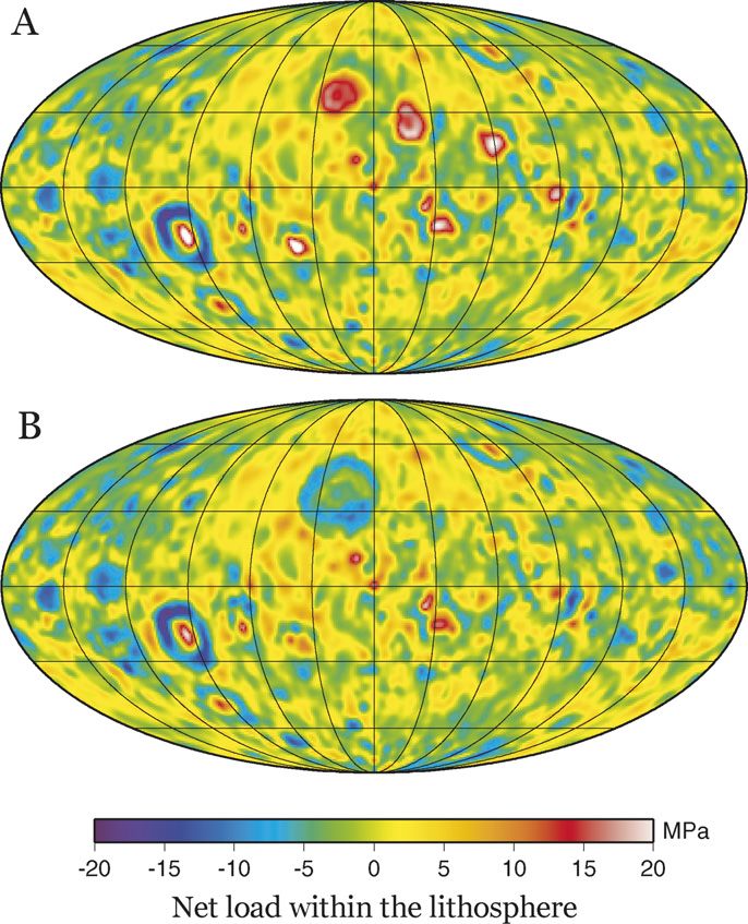
Crustal thickness of the Moon                                                   151

topography of this body is known globally with a relatively             2. Method
uniform spatial resolution (Smith et al., 1997; USGS, 2002;
Archinal et al., 2006), the synchronous rotation of the Moon                In this section we first describe the method by which we
has precluded the radio tracking of spacecraft over large por-          calculate the gravitational field of a body using arbitrarily
tions of the farside hemisphere. While the farside gravity field        shaped constant-density polyhedra. This is based on the work of
has been constrained by indirect means to a low precision (e.g.,        Werner and Scheeres (1997), and while we give a brief sketch
Konopliv et al., 2001), the spatial resolution of the nearside is       of the methodology here, the reader is referred to their paper for
considerably higher.                                                    further details. Given a forward modeling procedure for obtain-
   Previous investigations (e.g., Zuber et al., 1994; Neumann           ing the gravity field associated with a polyhedral shape model,
et al., 1996; Wieczorek and Phillips, 1998) have demonstrated           we next describe how one can invert for the shape of a poly-
that inversions for crustal thickness performed in the spherical-       hedron given an external gravity field. We note that a spatial
harmonic domain are unstable for the Moon as a result of the            inversion for the thickness of the lunar crust has been performed
exponential increase of errors that occurs when the Bouguer             both locally and globally by von Frese et al. (1997) and Potts
anomaly is downward continued to the crust–mantle interface.            and von Frese (2003a, 2003b), respectively. A major difference
To compensate for this, and to obtain reasonable solutions, this        with their approach is that they only modeled gravitational sig-
gravitational signature has been filtered (e.g., Phipps Morgan          natures that were correlated with the surface topography.
and Blackman, 1993). Filtering in the spherical-harmonic do-
main, however, does not take into account the dramatic lateral          2.1. Exterior gravitational field of a constant density
variations in quality of the lunar gravity data set. As one exam-       polyhedron
ple, Wieczorek and Phillips (1998) applied a filter with a value
of 0.5 at spherical-harmonic degree 30, whereas the resolution             By use of Gauss’ divergence theorem, the gravitational po-
of the nearside gravity field can reach almost degree 150. Thus,        tential external to a constant density object can be calculated
in order to obtain of global solution in the spherical-harmonic         either by an integral over its volume or surface:

domain, the global resolution was required to be close to the                            dV     Gρ        n̂ · r
                                                                        V = Gρ               =                     dS,              (1)
worst resolution of the gravity field, which is about degree 15                           r     2          r
(see Konopliv et al., 2001).                                                               V                     S
   To overcome this difficulty, we will invert for the crustal          where G is the gravitational constant, ρ is the density, r  is a
thickness of the Moon using a method developed in the spatial           vector from the observational point r to the differential volume
domain. In particular, we will employ the previously devel-             or surface element, and n̂ is the unit-normal vector of the sur-
oped method of Werner and Scheeres (1997) for calculating               face. If one assumes that the object can be approximated by a
analytically the exterior gravitational field of arbitrarily shaped     polyhedron, Werner and Scheeres (1997) have shown that the
constant-density polyhedra. For these computations we need to           right-hand side of Eq. (1) can be converted into two sums, one
know only the location of each vertex of the polyhedra, and the         over each of the edges of the polyhedron and the other over each
radii of these are constrained either by the known surface topog-       of its faces:
raphy or are inverted for at the crust–mantle interface in order              Gρ                                           B
to match the observed gravitational field. As benefits of this          V=              (r e · n̂A ) n̂A
                                                                                                       12 · r e + (r e · n̂B ) n̂21 · r e Le
                                                                                2
approach, the spatial resolution of the crustal thickness model                     edges
can be easily tailored where necessary, and when inverting for                     Gρ
                                                                               −        (r f · n̂f )2 ωf .                              (2)
the crust–mantle relief we can weight the misfit function by                        2
                                                                                         faces
the uncertainties associated with the observed gravity field. In
comparison to the spherical-harmonic inversions, however, the           Given this equation, it is straightforward to show that the grav-
benefits associated with this method come at the expense of a           itational acceleration (assumed to be positive when directed
considerable increase in computational burden.                          upwards) is given by
   In this paper we first describe how the gravitational field can      g ≡ ∇V
be computed from a polyhedral shape model and how the relief                                                B
along the crust–mantle interface can be inverted for utilizing             = Gρ            n̂A n̂A
                                                                                                 12 · r e + n̂B n̂21 · r e Le
the observed gravity and surface topography. Details concern-                      edges

ing these calculations are presented in Appendixes A and B.                    − Gρ             n̂f (n̂f · r f )ωf .                    (3)
Following this, we present our model results, describe how they                         faces
depend upon various assumptions, and compare with inversions
                                                                        Concerning the first sum in Eqs. (2) and (3), which is performed
performed in the spherical-harmonic domain. Finally, we dis-            over all edges of the polyhedron, n̂A and n̂B are the unit-normal
cuss the global features of our model, compare our predictions          vectors of two faces that are connected by a single edge. If we
with the available seismic constraints, quantify the structure of       define r 12 as the vector pointing from vertex r 1 to vertex r 2 of
the most prominent impact basins, and estimate the magnitude            this edge, then the unit vectors n̂A        B
                                                                                                           12 and n̂21 are defined as
of the load the lithosphere is currently supporting beneath the
basins.                                                                 n̂A
                                                                          12 = r̂ 12 × n̂A ,
152                                            H. Hikida, M.A. Wieczorek / Icarus 192 (2007) 150–166

n̂B
  21 = n̂B × r̂ 12 .                                               (4)
r e is a vector from the observation point to any point on the line
made by the two vertices r 1 and r 2 , of which we choose r 1 for
this study. Le is the function
          a+b+e
Le = ln         ,                                                  (5)
          a+b−e
where a and b are the distances from the observation point to
vertex r 1 and r 2 , respectively (i.e., a = re ), and e is the edge
length r12 .
    The second summation in Eqs. (2) and (3) is performed over
all faces of the polyhedron. Here, n̂f is the unit-normal vector
of a given face, and r f is a vector from the observation point
to any point in the plane of this face. In this study, each face
will be a triangular patch defined by three vertices r 1 , r 2 , and
r 3 ordered counterclockwise about the face normal n̂f , and the
vector r f will be allocated to the vertex r 1 . Finally, ωf is a
solid angle associated with each face given by
                                                                            Fig. 1. Schematic illustration of our polyhedral shape model of the Moon. Each
             β                                                              layer has a constant density and the vertical gravitational acceleration is calcu-
ωf = 2 arctan ,                                                    (6)      lated at an altitude of 30 km above the average surface radius.
             α
where
                                                                            (ρcore − ρmantle ), we will then invert for the shape of a polyhe-
α = |r 1 − r||r 2 − r||r 3 − r| + |r 1 − r|(r 2 − r) · (r 3 − r)            dron whose surface corresponds to the crust–mantle interface
                                                                            using a density (ρmantle − ρcrust ).
      + |r 2 − r|(r 3 − r) · (r 1 − r)                                          In this investigation, we model only the radial gravitational
      + |r 3 − r|(r 1 − r) · (r 2 − r),                            (7)      field of the Moon. Since we will sample the gravitational field
                                                                            derived from a spherical-harmonic model of the gravitational
β = (r 1 − r) · (r 2 − r) × (r 3 − r).                             (8)      potential on a set of grid points (and not use direct line-of-
We note that both the numerator and denominator of the argu-                sight observations), it is straightforward to show that the ra-
ment for the arctan function is signed and must be taken into               dial gravitational component contains all information of the
account when computing this value. The reader is referred to                spherical-harmonic model. Modeling the other two components
Figs. 3, 5, 6, and 7 of Werner and Scheeres (1997) for a more               would only introduce redundant constraints. In practice, the ra-
complete description of the geometry and notation of the above              dial component of the gravity field will be calculated on a set
vectors and quantities. We note that for a given polyhedron, all            of grid points on the surface of a sphere 30 km above the mean
unit vectors in Eqs. (2) and (3) only needed to be computed                 planetary radius, which corresponds to the average altitude of
once, whereas r e , Le , r f , and ωf need to be recomputed for             the Lunar Prospector spacecraft during its extended mission
each observation point.                                                     (see Konopliv et al., 2001).
                                                                                In order to invert for the shape of the crust–mantle interface,
                                                                            it will be assumed that the densities of the crust, mare basalts,
2.2. Inversion strategy
                                                                            mantle, and core are known. Furthermore, we will assume a
                                                                            core radius, and use known models of the lunar shape, mare
    The previous section described how one could calculate the
                                                                            thickness, and gravitational field sampled on an appropriate grid
gravitational field of a constant density body by approximat-
                                                                            (see Section 3). With these assumptions, the only unknowns that
ing its shape in terms of a polyhedron. In this section, we
                                                                            remain are the radii of the vertices that comprise the polyhedral
will describe how one can conversely invert for the shape of
                                                                            model of the crust–mantle interface, (r1 , r2 , . . . , rN ). We define
a polyhedron given knowledge of the external gravity field. In
                                                                            the misfit between the observed and calculated radial gravity,
particular, for our investigation of crustal thickness variations,
                                                                            weighted by the uncertainty of the observed gravity σ , on a set
we will assume that the structure of the Moon can be described              of N grid points (θi , φi ) as
by possessing a crust, mare basalts, mantle and core, all hav-
                                                                                                          N
ing constant densities (see Fig. 1). We will first calculate the                                        1  giobs − gi (r1 , r2 , . . . , rN ) 2
gravitational field of a polyhedron with density ρmare that corre-          f (r1 , r2 , . . . , rN ) =                                          , (9)
                                                                                                        N                σi
sponds to the known shape of the Moon. Next, the gravitational                                               i=1
attraction of a polyhedron with density (ρmare − ρcrust ) will              where
be subtracted from this using the shape of the Moon with the
thickness of the mare basalts removed. After adding the grav-               gi (r1 , r2 , . . . , rN )
                                                                                      topo
itational contribution of a small spherical core with a density                 = gi         + gimare + gimantle (r1 , r2 , . . . , rN ) + g core .     (10)
Crustal thickness of the Moon 153
All gravitational accelerations are calculated at the same radius Table 1
of observation, Robs . Parameters and properties of the polyhedral crustal thickness model
The goal at this point is to find those radii of the mantle poly- Parameter Symbol Value Unit
hedral model, (r1 , r2 , . . . , rN ), that minimize the misfit function GM GM 4902.80295 × 109 m3 s−2
Eq. (9). For this purpose, we use the Polak–Ribière conjugate Mean planetary radius R 1737.1 km
gradient method (see Press et al., 1992, chap. 10), which is an Observational radius Robs 1767 km
efficient algorithm for finding the nearest local minimum of Density of crust ρcrust 2800 kg m−3
Density of mare basalts ρmare 3100 kg m−3
a multi-dimensional function. This method requires computa-
Density of mantle ρmantle 3360 kg m−3
tion of the gradient of the misfit function, and uses conjugate Core radius Rcore 370 km
directions instead of the local gradient in order to iteratively Density of core ρcore 6600 kg m−3
approach the minimum misfit. The components of the gradient Average crustal thickness – 43 km
matrix are given by Minimum crustal thickness –154 H. Hikida, M.A. Wieczorek / Icarus 192 (2007) 150–166
ness is consistent with the range of 49 ± 16 km advocated
by Wieczorek et al. (2006) that is based upon a variety of
gravity, topography, and seismic considerations. Furthermore,
while our utilized core density and radius are certainly not
unique, we note that our adopted values are generally con-
sistent with a number of recent geophysical and geochemical
investigations (e.g., Konopliv et al., 1998; Hood et al., 1999;
Williams et al., 2001; Kuskov et al., 2002; Righter, 2002;
Khan et al., 2004, 2006; Khan and Mosegaard, 2005; Lognonné
and Johnson, 2007).
Concerning the average crustal thickness, we note that we
could have chosen this value such that our inversion results
matched those obtained from analyses of the Apollo seismic
data. While the original analysis suggested a crustal thickness
of about 60 km in the vicinity of the Apollo 12 and 14 stations
(Toksöz et al., 1974), recent analyses point to thinner values for
the region of the Apollo seismic network of 45 ± 5 km (Khan et
al., 2000), 38±3 km (Khan and Mosegaard, 2002), and 30±2.5
(Lognonné et al., 2003). Given the large spread of these esti-
mates, we have not attempted to fit any specific model.
We next describe how we defined the coordinates used in
the polyhedral shape models of the surface and crust–mantle
interface. For each, we started with a regular icosahedron of 20
equilateral triangular patches. Each triangular patch was then
recursively subdivided into 4 subtriangles until a desired spatial
sampling was achieved (see Appendix A for further details). For
the surface model, we divided each of the original 20 triangu-
lar faces into 45 faces, giving rise to a total of 20,480 faces and
10,242 vertices. The angular distance of each edge in this model
is about 2 degrees, which corresponds to about 60 km on the lu-
Fig. 2. Crustal thickness of the Moon derived from a polyhedral shape model
nar surface and a spherical-harmonic resolution close to degree inversion. (A) Crustal thickness excluding mare fill. The location of each vertex
100. This corresponds approximately to the inherent spatial res- of the polyhedral model of the crust–mantle interface is shown as solid dots.
olution of the employed Clementine shape model of the Moon. (B) The difference between the observed and modeled radial gravity. Images
Each vertex was then assigned an absolute radius based on the are shown in a Mollweide projection with a central meridian of 0◦ longitude.
359-degree spherical-harmonic model USGS359 (USGS, 2002;
Wieczorek, 2007). This model is based upon a combination of eled radial gravity. We use the latitude and longitude points of
Clementine altimetry data and stereo photogrammetry over the this model when calculating the misfit function of Eq. (9).
lunar poles and possesses a significantly higher spectral correla- In generating our final crustal thickness model, we used
tion with the observed gravity field than the previous spherical- the parameter values given in Table 1 and the mare basalt
harmonic model GLTM2C (Smith et al., 1997). thickness model that was employed by Wieczorek and Phillips
For our shape model of the crust–mantle interface, we ini- (1998), which is the mare basalt disk model of Solomon and
tial started by subdividing each of the 20 faces of a regular Head (1980) revised by the maximum thickness estimates of
icosahedron into 144 triangular patches, leading to a total of Williams and Zuber (1998). Furthermore, we used the lu-
2880 triangular patches and 1442 vertices. The average dis- nar shape model USGS359, the lunar gravity model LP150Q
tance between vertices is about 180 km, corresponding to a (Konopliv et al., 2001), and the gridded radial gravity uncer-
spherical-harmonic resolution of about 37. We note that the pre- tainties from the model JGM100J1. The spherical-harmonic
vious models of Wieczorek and Phillips (1998) and Wieczorek representations of the gravity and topography were truncated
et al. (2006) filtered the Bouguer anomaly using a filter with beyond degree 90, as this corresponds approximately to the av-
a value of 0.5 at degree 30, demonstrating that our model has erage resolution of the topography model.
a higher spatial resolution. Experience has shown that this ini- Our final model is shown in Fig. 2A, where, for plotting
tial grid for the crust–mantle interface was not sufficient to fit purposes, we have used the GMT command surface (with
everywhere the gravity field on the nearside of the Moon. In or- T = 0.25; Smith and Wessel, 1990) to interpolate between ver-
der to rectify this, we have increased the spatial resolution in tices. Also shown are the locations of the vertices used in our
the vicinity of the major impact basins and in regions where the crust–mantle shape model. In Fig. 2B, we plot the difference
crustal thickness changes rapidly. Furthermore, the resolution between the observed and modeled radial gravity. The average
was increased over some regions on the nearside that originally misfit for the nearside is seen to be about 15 mGals, whereas for
gave rise to large differences between the observed and mod- the farside it is somewhat larger, about 30 mGals, with some re-Crustal thickness of the Moon 155
gions possessing differences up to 240 mGals. We note that the
estimated errors in the radial component of the employed gravi-
tational field are about 30 mGals for the nearside, and can reach
up to 200 mGals for the farside (Konopliv et al., 2001). We es-
timate the uncertainties associated with our crustal thickness
model utilizing the first-order Cartesian Bouguer slab formula
(e.g., Turcotte and Schubert, 1982)
g = 2πG(ρmantle − ρcrust ) h, (12)
where h is the magnitude of relief at the crustal–mantle in-
terface with a density contrast of (ρmantle − ρcrust ). Using our
average nearside and farside data misfits of 15 and 30 mGal,
we find that this corresponds to an uncertainty of about 0.5 and
1 km of mantle relief, respectively.
For comparative purposes, we have also calculated a crustal
thickness model using the filtered spherical-harmonic inversion
methodology of Wieczorek and Phillips (1998) with the same
parameters as adopted for our polyhedral model. We have ap-
plied the same filter to the Bouguer anomaly as used in that
paper, and plot this model in Fig. 3A. While the models are
generally similar, as shown in Fig. 3B, the fit to the observed
radial gravity is poorer than ours. Histograms of the differ-
ence in crustal thickness between these two models is shown
in Fig. 4 over both the lunar near- and far-side hemispheres.
The model differences over the nearside are most certainly a
result of the filtering operation that was used to stabilize the
spherical-harmonic inversion. While the standard deviation be-
tween the two models over this hemisphere is only about 3 km,
important differences are evident where the crustal thickness
changes rapidly, and can be as high as almost 20 km in some
Fig. 3. Crustal thickness of the Moon derived from a filtered spherical-harmonic
regions. In contrast, the larger differences that are found over inversion using the same parameters as in Fig. 2. (A) Crustal thickness ex-
the farside hemisphere are primarily a result of our model being cluding mare fill. (B) The difference between the observed and modeled radial
smoother there, which is a direct consequence of having taken gravity.
into account the uncertainties in the gravity field. The large os-
cillations evident in the filtered spherical-harmonic inversion the gravitational attraction of mare basalts with thickness hmare
are most likely a result of the amplification of measurement and density contrast (ρmare − ρcrust ) to that of crust–mantle re-
noise. lief h of density contrast (ρmantle − ρcrust ), which yields the
Finally, we address some of the model dependencies associ- relationship
ated with our chosen set of input parameters. First, concerning ρmare − ρcrust
the fidelity of the topography model, we have also performed h= hmare . (13)
a crustal thickness inversion using the GLTM2C spherical- ρmantle − ρcrust
harmonic model. While the USGS359 model is preferred (see Using densities of 2800, 3100 and 3360 kg m−3 for the crust,
Wieczorek, 2007), in part because it includes data over the poles mare basalts, and mantle, respectively, each kilometer of mare
obtained by stereo imaging, the difference in crustal thickness basalts is seen to correspond to a change of about 0.5 km of
between the two is on average only 1.5 km. Nevertheless, in mantle relief. In the extreme situation where we were to have
some regions, particularly over the poles, the difference can over- or under-estimated the mare basalt thickness by 6 km, the
be more substantive, up to 12 km. Other regions with large total crustal thickness would only change by about 3 km. Fur-
differences correspond to gaps in the Clementine altimetry thermore, the total crustal thickness excluding the mare basalts
data and are related to different interpolation schemes used in would also only change by about 3 km. Thus, for most pur-
constructing the USGS359 and GLTM2C models. Tests using poses, any errors introduced into our crustal thickness model
the entirely photogrammetric topographic model ULCN2005 by the use of an inappropriate mare thickness model are rela-
(Archinal et al., 2006), which possesses a higher spatial resolu- tively unimportant.
tion and more even data coverage, yields results that are nearly Finally, we note that Wieczorek and Phillips (1998, 1999)
identical to those based on USGS359. utilized a model of crustal structure that was stratified into up-
Another source of error is related to our adopted mare per anorthositic and lower noritic layers. Such a model was
basalt thickness model, and we evaluate this using the Carte- based on the possible existence of an intracrustal seismic dis-
sian Bouguer slab formula. With this approximation, we equate continuity about 20 km below the surface (e.g., Toksöz et al.,156 H. Hikida, M.A. Wieczorek / Icarus 192 (2007) 150–166
Fig. 4. Histograms of the difference in crustal thickness between the polyhedral and filtered spherical-harmonic inversions. The standard deviation over the near-
and far-side hemispheres is 3 and 4 km, respectively.
1974), the mafic composition of some central peaks that are dependent estimates as to the magnitude of lateral variations in
derived deep below the surface (Tompkins and Pieters, 1999; density, we cannot easily account for this in our models.
Wieczorek and Zuber, 2001), the mafic character of the floor Our crustal thickness model is considerably smoother over
of the South Pole–Aitken basin (Pieters et al., 1997), the com- the farside hemisphere than previous spherical-harmonic based
mon interpretation that the mafic impact melts were derived models. This, however, is most likely a consequence of our
from the lower crust, and the relationship between the lunar having taken into account the larger gravitational uncertain-
geoid and topography over the lunar highlands (Wieczorek and ties there, and is not necessarily real. Direct gravitational con-
Phillips, 1997). While more complicated crustal thickness mod- straints over the farside, as will be obtained from the upcoming
els that take into account vertical variations in density might Japanese mission SELENE (Kato et al., 2007), will be nec-
differ somewhat from the model presented here, Wieczorek and essary to investigate shorter wavelength features that might
Phillips (1998) noted that the difference in total crustal thick- be present there. In contrast to the farside hemisphere, rela-
ness between their single and dual-layered models was not too tive variations in crustal thickness are somewhat larger for our
great (the standard deviation between the two is only about model over the nearside than previous models, particularly be-
4 km). neath the giant impact basin (see Section 4.3 and Fig. 6). This
is simply a result of short wavelength features having been
4. Discussion damped by the filtering procedure used in previous spherical-
harmonic based models.
4.1. Global structure The minimum crustal thicknesses in our model, after ex-
cluding the mare basalt fill, are found within the Orientale and
Our crustal thickness model shares the same general at- Crisium basins with values of 0.7 and 0.8 km, respectively. Pre-
tributes that have been noted by previous investigators (Zuber et vious models based on filtered spherical-harmonic inversions
al., 1994; Neumann et al., 1996; Wieczorek and Phillips, 1998; obtained minimum crustal thicknesses close to zero only be-
Potts and von Frese, 2003a; Wieczorek et al., 2006). In partic- neath the Crisium basin. Though our model was constructed by
ular, the crust is seen to be substantially thinned beneath many requiring the minimum thickness to be close to zero, these two
of the large impact basins, and some of these are surrounded basins, nevertheless, should be considered as good candidates
by rings of thickened crust. The structure of the giant impact for having potentially excavated all the way through the crust
basins will be discussed in greater detail in Section 4.3. and into the mantle. Given our uncertain knowledge of lateral
As a result of our assumption of a constant density crust, the variations in crustal and mantle density, the average thickness
higher elevations associated with the lunar farside hemisphere of the crust, the thicknesses of the mare basalts, and uncertain-
give rise to a thicker crust there. The axis of the thickened ties in the gravity model, it is probably reasonable to expect that
crust points towards (7◦ N, 156◦ W), and the average hemi- our crustal thickness model possesses absolute uncertainties on
spheric crustal thickness difference with respect to this axis the order of 5 km. Using this number as a guide, not only could
is 7.4 km. The direction of this hemispheric variation coin- have the Orientale and Crisium basins excavated into the man-
cides approximately with the Earth–Moon axis, and hence can tle, but so could have Humorum and Humboldtianum.
be described approximately as a nearside–farside crustal thick-
ness dichotomy. Nevertheless, as discussed in Wieczorek et al. 4.2. Comparison with seismic constraints
(2006), if lateral variations in crustal and mantle density exist
between the near- and far-side hemispheres, these might act to Our crustal thickness model was constructed based on as-
reduce the magnitude of such an effect. Several lines of evi- sumptions about the crustal and mantle density, combined with
dence exist suggesting that the two hemispheres are somewhat the constraint that the minimum crustal thickness (excluding
compositionally distinct (see Jolliff et al., 2000), but lacking in- mare basalt fill) is close to zero. As no seismic informationCrustal thickness of the Moon 157
Fig. 5. Comparison of the crustal thicknesses obtained from a polyhedral shape model inversion and the seismic results of Chenet et al. (2006). The first four sites
correspond to the Apollo stations 12, 14, 15 and 16, and the rest are for meteoroid impacts.
was input into our model, we here quantify how well our model stations. In order to make their inversion tractable, it was neces-
compares to the available seismic constraints. Such constraints sary to assume that the seismic velocity of the crust and upper
include estimates of the crustal thickness in the vicinity of the mantle was everywhere the same, for which they used the av-
Apollo 12 and 14 stations, the region of the Apollo seismic net- erage velocities from the model of Gagnepain-Beyneix et al.
work, and at a variety of meteoroid impact sites. (2006). The differences between observed and predicted first
We first note that the original analysis of the Apollo seis- arrival times were then modeled by variations in crustal thick-
mic data suggested a crustal thickness of about 60 km (Toksöz ness. Crustal thickness estimates were obtained at 25 locations,
et al., 1974) for the Apollo 12 and 14 landing sites, which lie including 2 artificial impact sites, 19 meteoroid impacts, and
within about 155 km of each other. Our model, in contrast, pre- the 4 Apollo stations. These sites are generally located on the
dicts a thinner average crustal thickness at these two sites of nearside of the Moon, though a few of the most distant impacts
about 40 km. Recent analyses of the seismic data suggest that are located beyond the lunar limbs.
the crustal thickness in the region of the Apollo seismic network In Fig. 5, we compare the crustal thicknesses obtained from
is probably considerably thinner than once though. Khan et al. our polyhedral model to the seismic results of Chenet et al.
(2000) and Khan and Mosegaard (2002) first proposed values of (2006). The site numbers correspond to those in Tables 2 and
45 ± 5 km and then 38 ± 3 km that should be taken as being rep- 3 of that paper, and here we only note that the first 4 sites corre-
resentative of the area surrounding the Apollo seismic network, spond to the Apollo 12, 14, 15 and 16 stations, respectively. The
which includes Apollo 12, 14, 15, and 16. In a similar analy- two models are broadly consistent, with 17 of the 25 sites being
sis, Lognonné et al. (2003) obtained a value of 30 ± 2.5 km, within one standard deviation of each other. In particular, we
though it should be noted that this estimate places somewhat note that the reduced chi-squared misfit of the two distributions
more emphasis on the structure beneath the Apollo 12 station. is equal to 1.18, whereas the expected value should be 1 ± 0.29
An analysis by Chenet et al. (2006) obtained an average of (e.g., Press et al., 1992). Nevertheless, a few locations compare
34 ± 7 km for the four Apollo stations using the seismic veloc- poorly. In particular, we predict somewhat higher crustal thick-
ity model of Gagnepain-Beyneix et al. (2006) combined with nesses for the Apollo landing sites, and the Apollo 16 station
the artificial and natural impact events (see below). Our inver- and impact site 24 are somewhat discordant. It is important to
sion predicts an average value of about 44 km beneath the four note that the crustal thickness estimates of Chenet et al. (2006)
Apollo seismic stations, which is generally compatible with, are dependent on the crustal and mantle velocities that were em-
though somewhat higher than, these recent analyses. ployed in their inversion and that different values might perhaps
In addition to the seismic studies mentioned above, one in- give a better fit.
vestigation has attempted to place constraints on the crustal
thickness at the Apollo 16 site. Goins et al. (1981) performed 4.3. Impact basin structure
an analysis of putative converted phases at this site and obtained
a crustal thickness of 75 km. In contrast, our model predicts a As is clearly visible in Fig. 2, the most dramatic crustal
crustal thickness of 54 km. The recognition of converted phases thickness variations on the Moon are associated with large im-
at this site is somewhat contentious (Chenet et al., 2006), and pact basins. In this section we characterize the structure of both
the reported crustal thickness estimate is clearly inconsistent young and old impact basins, and estimate the size of their ex-
with our model. cavation cavities—that portion of the crust that was ballistically
The only study that has attempted to place constraints on the excavated during the cratering process. Our methodology par-
crustal thickness far from the Apollo seismic network is that of allels closely that of Wieczorek and Phillips (1999) in that the
Chenet et al. (2006). In their study, seismic signals induced by geometry of the excavation cavity will be approximated to first
artificial and natural meteoroid impacts were used to constrain order by restoring the uplifted crust–mantle interface beneath
the crustal thickness beneath both the impact sites and Apollo these basins to its (assumed horizontal) pre-impact position; the158 H. Hikida, M.A. Wieczorek / Icarus 192 (2007) 150–166
Fig. 6. Azimuthally averaged crustal thickness profiles of the major young impact basins. Vertical axes are radial distance from the center of the Moon, and horizontal
axes are the radial distance from the center of each basin. Black colored regions represent mare fill, the upper solid line is the surface topography, the subsurface
solid line is the crust–mantle interface from the polyhedral inversion, and the dashed line is the crust–mantle interface obtained from the filtered spherical-harmonic
inversion. Age classification using the notation of Halekas et al. (2003) and the center of the basin are indicated. All plots possess the same scale.
reader is referred to that paper for a more detailed discussion. Radially averaged basin profiles are shown in Fig. 6 for these
Knowledge of the size of the excavation cavity can be used to basins using both our polyhedral (solid lines) and spherical-
estimate various quantities such as the depth of excavation, the harmonic based (dashed lines) crustal thickness models. These
transient cavity radius, and the mass and volume of excavated are plotted in reverse order of their reconstructed excavation
materials. cavity diameter, as determined below, and the age classifica-
We will first discuss those basins with good gravity coverage tion following the numbering scheme of Halekas et al. (2003)
that are as young or younger than Smythii [i.e., age group 5 of is indicated (groups of impact basins increase in age from 1 to
Wilhelms (1987), see also Wilhelms (1984)] and which have di- 15, and the number is preceded by I, N, or P, signifying Im-
ameters larger than 365 km (the approximate resolution of the brian, Nectarian, or pre-Nectarian, respectively). While the two
crustal thickness model). Of these basins, two are Imbrian in
crustal thickness models are generally similar, the amount of
age (Imbrium and Orientale), six are Nectarian (Serenitatis, Cri-
predicted uplift of the crust–mantle interface beneath the Hu-
sium, Humorum, Humboldtianum, Mendel–Rydberg, and Nec-
morum, Orientale, Humboldtianum and Cruger–Sirsalis basins
taris), and two are pre-Nectarian (Grimaldi and Smythii). The
Cruger–Sirsalis basin (Cook et al., 2002) will additionally be is clearly larger for our polyhedral model.
considered because of its remarkable crustal thinning. Although As discussed in Wieczorek and Phillips (1999), we will as-
the relative age of this basin is not well known, it appears to be sume that the crust mantle interface rebounded in a purely
younger than the Grimaldi basin, but older than the Orientale vertical fashion following the excavation stage of the cratering
basin (Paul Spudis, personal communication). The centers for process. We assume that the crust–mantle interface was orig-
most basins were taken from the geologic mapping of Wilhelms inally flat, here approximated by the average depth at three
(1987), with the exceptions of Orientale, Imbrium, Humbold- excavation cavity radii, and simply “restore” this interface to its
tianum and Cruger–Sirsalis that were estimated from our crustal original presumed horizontal pre-impact position by a vertical
thickness model. translation. The resulting cavity, which is generally parabolic,Crustal thickness of the Moon 159
Table 2
Reconstructed excavation cavity measurements for the young nearside impact
basins
Basin Age Polyhedral model Filtered spherical
harmonic inversion
Diameter Depth Diameter Depth
(km) (km) (km) (km)
Grimaldi P-7 206 ± 4 18.1 ± 1.7 204 ± 6 14.7 ± 1.8
Cruger–Sirsalis – 306 ± 20 27.8 ± 5.1 392 ± 20 15.8 ± 2.2
Mendel–Rydberg N-6 337 ± 13 29.4 ± 2.9 302 ± 10 28.4 ± 2.9
Humorum N-4 382 ± 6 33.4 ± 1.3 431 ± 15 29.0 ± 1.7
Orientale I-1 383 ± 5 46.9 ± 1.6 418 ± 8 38.4 ± 1.4
Humboldtianum N-4 394 ± 18 33.0 ± 3.6 486 ± 34 26.8 ± 4.2
Nectaris N-6 455 ± 5 34.9 ± 1.9 468 ± 10 30.3 ± 1.3
Crisium N-4 560 ± 2 34.6 ± 3.7 611 ± 15 35.3 ± 2.2 Fig. 7. Reconstructed excavation cavity depth as a function of its diameter.
Smythii P-11 567 ± 19 36.5 ± 1.5 580 ± 14 35.4 ± 1.3 Best fit line excluding the two largest basins (Imbrium and Serenitatis) is
Serenitatis N-4 718 ± 22 28.8 ± 3.9 745 ± 5 30.5 ± 2.4 hex = (0.083 ± 0.002)Dex . The shaded area is the range of ambient crustal
Imbrium I-3 895 ± 11 21.1 ± 3.7 901 ± 5 23.5 ± 1.8 thicknesses for these basins at three excavation cavity radii.
is assumed to approximate the first order geometry of the basin Fig. 7 plots the depth–diameter relationship of the recon-
excavation cavity. structed excavation cavity for the 11 basins shown in Fig. 6.
In order to estimate the depth and diameter of the excava- For reference, the ambient crustal thickness surrounding these
tion cavity, we employ two methods. First, we simply fit the basins at three excavation cavity radii is shown by the shaded
shape of the depression using a parabolic function, from which region in this plot. With the exception of the two largest basins
the depth and diameter are easily obtained. Since some basins (Imbrium and Serenitatis), the depth of excavation generally in-
are poorly approximated by a parabolic form, we also estimate creases with increasing excavation cavity diameter. Excluding
the depth and diameter using the depth at the basin center and Imbrium and Serenitatis, the best fit straight line (constrained
the diameter at which the excavation cavity is first equal to the to pass through the origin) is found to be hex = (0.083 ±
surrounding average surface elevation. Here, we quote the av- 0.002)Dex , where hex and Dex are the depth and diameter of the
erage from these two methods and the “uncertainty,” which is excavation cavity, respectively. This result is generally consis-
half of their difference, in Table 2. Finally, concerning the depth tent with craters ranging in size from centimeters to several tens
estimates, we added in quadrature the uncertainty in crustal of kilometers in diameter which all yield depth/diameter ra-
thickness that is expected from the uncertainty in the gravity tios of the excavation cavity close to 0.1 (Croft, 1980; O’Keefe
field [see Eq. (12)]. and Ahrens, 1993). We note that Wieczorek and Phillips (1999)
We note that this method of reconstructing the excavation originally obtained a depth/diameter ratio of 0.115 ± 0.005 us-
cavity ignores several processes and complications, but that ing this same methodology, which is slightly larger than our
these are likely to have magnitudes that are comparable to estimate. This is related primarily to their having used the
the uncertainties associated with our crustal thickness model. Apollo-era seismic constraint of 60 km at the Apollo 12 and
In particular, gravitational collapse of the crater wall would 14 sites in constructing their crustal thickness model, which is
tend to increase its diameter, and this methodology would now recognized to be too large.
thus overestimate the excavation cavity diameter. Neverthe- We briefly comment on the apparently anomalous excava-
less, it has been noted that the relative importance of wall tion cavities of the Imbrium and Serenitatis basins. As dis-
collapse appears to decrease with increasing crater diameter cussed by Wieczorek and Phillips (1999, 2000), these basins ap-
(Pike, 1976). If some of the basin ejecta were to fall back pear to have impacted into an anomalous geochemical province
into the crater, this method would slightly underestimate the rich in incompatible elements, a region now referred to as
excavation depth. The biggest uncertainty with this method- the Procellarum KREEP Terrane (see also Jolliff et al., 2000;
ology concerns the fact that the excavation flow field set up Korotev, 2000). The Imbrium basin clearly resides within the
during the excavation stage will displace some crustal mate- confines of this province, whereas the Serenitatis basin borders
rials radially away from their original position (Melosh, 1989; this and the adjacent Feldspathic Highlands Terrane. Thermal
O’Keefe and Ahrens, 1993). We can not easily quantify this ef- evolution models based on reasonable geochemical constraints
fect, but suspect that this will not dramatically affect our results. (Wieczorek and Phillips, 2000) suggest that the heat flow within
The effects of viscous relaxation and having excavated through the Procellarum KREEP Terrane could have been several times
the entire crust will be discussed later. Finally, we note that the larger than that of the surrounding regions. Thus, it is plausible
presence of an impact melted crust and/or mantle below the ex- that high temperatures could have led to enhanced rates of vis-
cavation cavity will not affect our geometric reconstructions as cous relaxation, leading to the slow lateral transport of crustal
long as this material does not flow laterally from its pre-impact materials into the basin center. Nevertheless, as shown by Mohit
position. Even if our reconstructed depths and diameters were and Phillips (2006), viscous relaxation, even in the presence of
to be systematically biased by a small factor, to first order, this a hot crust, is difficult to achieve for regions where the crust is
should affect all craters equally. thin.160 H. Hikida, M.A. Wieczorek / Icarus 192 (2007) 150–166
Fig. 8. Azimuthally averaged crustal thickness profiles for the major pre-Nectarian impact basins. Basin centers taken from Wilhelms (1987).
Alternatively, as discussed by the same authors, it is possi- fully crystallized. Higher temperatures at this time could have
ble that the lunar magma ocean had not completely crystallized plausibly given rise to the viscous relaxation of any crustal
beneath the Procellarum KREEP terrane at the time of these thickness variations that might originally have been present (see
impacts (3.89 ± 0.01 Ga for Serenitatis, Dalrymple and Ryder, Mohit and Phillips, 2006). From a geophysical standpoint, it
1996; 3.85 ± 0.02 Ga for Imbrium, Ryder, 1994). It has long thus appears that the rheologic behavior of the crust was sig-
been recognized that the last remaining dregs of the magma nificantly different before the Smythii impact event than after-
ocean could have remained molten for about a billion years as a wards. This is almost certainly related to the thermal regime
result of its high concentration of incompatible elements (e.g., that these basins were subjected to shortly after the formation
Solomon and Longhi, 1977; Wieczorek and Phillips, 2000). of the crust, and if the absolute ages of these basins could be
If the Imbrium and Serenitatis basins excavated all the way determined, this fact could be used to place constraints on the
through the crust, this magma, if present at these locales, could early thermal evolution of the Moon.
have flown into the excavation cavities of these two basins. If Finally, it is noted that the crust–mantle interface beneath the
the solidified magma had a density similar to that of the crust, Nectaris, Crisium, and Smythii basins appears to be horizontal
such a phenomenon would artificially reduce the reconstructed in the central portion of these craters. Furthermore, the crustal
excavation depths of these basins using our methodology. thickness is predicted to be fairly thin at these locations, less
The crustal structure of basins that are older than those con- than about 10 km. Such a structure could arise if these basins
sidered above, and which should be resolved in our crustal excavated all the way through the crust and into the mantle, and
thickness model, are shown in Fig. 8. While the absolute ages of if for some reason we were systematically overestimating the
these basins are unknown, stratigraphically they are older than crustal thickness in these regions. By choosing different values
the Nectaris basin, which is believed by many to have formed for the crustal and mantle densities, at least locally, it is proba-
at 3.93 Ga (e.g., Spudis, 1993), though an age as old as 4.1 ble that crustal thickness inversions could be obtained where the
Ga is possible (e.g., Haskin et al., 1998; Korotev et al., 2002). crust was nearly absent beneath these craters. If these craters did
As is seen, the crust–mantle interface beneath these basins is excavated though the entire crust, then our reconstructed exca-
relatively flat, and if any crustal thinning is present, this is gen- vation cavity depths should be considered as minimum values.
erally restricted to variations of less than 10 km. Since there is
no reason why these impact basins would not also have exca- 4.4. Isostatic state of lunar impact basins
vated deeply into the crust, their lack of any significant crustal
thinning is most likely attributable to post-impact modification Large positive gravity anomalies on the Moon, referred to
processes. as “mascons,” were discovered at the centers of many basins
Given the old pre-Nectarian ages of these basins, it is likely during the Apollo era (Muller and Sjogren, 1968). A common
that the crust was hotter when they formed than it was for the explanation for this observation is that (1) the impact basins
basins younger than Smythii. Indeed, for the oldest of these were initially in a state of isostatic equilibrium, and (2) when
basins, it is possible that the magma ocean had not yet even the mare basaltic lava flows erupted hundreds of millions ofCrustal thickness of the Moon 161
years later, the lithosphere was thick enough to support the
stresses associated with these loads over geologic time (e.g.,
Solomon and Head, 1980; Bratt et al., 1985).
While the mare basalts certainly contribute to the observed
gravitational signature of these basins, it has been suggested
that the mascons might instead have their origin primarily in
the uplift of the crust–mantle interface beneath these basins
(Neumann et al., 1996; Wieczorek and Phillips, 1999). This
hypothesis requires the mantle uplift to be superisostatic (i.e.,
uplifted beyond its natural isostatic position), and in support of
this interpretation, Konopliv et al. (2001) have identified several
mascon basins that do not appear to show evidence for mare
volcanism. In this context, it should be noted that the largest
expanse of mare volcanism, Oceanus Procellarum, shows no
significant positive gravitational anomaly.
In this section, we quantify the isostatic state of the young
nearside basins as is implied by our crustal thickness model.
The net load acting on the lithosphere is calculated according
to the equation (e.g., Belleguic et al., 2005)
q = g0 ρcrust h1 + (ρmantle − ρcrust )h2 + (ρmare − ρcrust )hmare ,
(14)
where g0 is the gravitational acceleration at the lunar surface,
h1 is the surface relief referenced to the geoid at the mean
radius of the Moon, and h2 is the amount of mantle uplift ref-
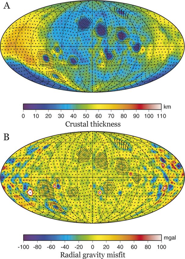
erenced to an equipotential surface at the mean radius of the Fig. 9. The net load acting on the lithosphere (A) with and (B) without the
crust–mantle interface. The first term accounts for the load due contribution of the mare basalts.
to surface topography, the second is the load resulting from re-
lief along the crust–mantle interface, and the third is the load of cale, or that the load associated with these lavas gave rise to a
the mare basalts. The shape of the equipotential surfaces at the small amount of lithospheric flexure.
mean surface radius and crust–mantle interface were estimated Some basins such as Orientale, Nectaris, Smythii, and Hum-
using first order theory, and the contribution resulting from the boldtianum, are still seen to be supporting a downward directed
centrifugal and tidal potentials was explicitly taken into consid- lithospheric load, even after the load of the mare basalts is re-
eration. moved. These excess loads are plausibly interpreted as resulting
Fig. 9A shows our estimated vertical load that is acting on from superisostatic uplift of the mantle that could have oc-
the lunar lithosphere (positive stresses are directed downward). curred as the basin floor rebounded following the excavation
As is seen, large portions of the lunar crust are consistent with stage of crater formation (see Neumann et al., 1996; Wieczorek
being isostatic (i.e., the net load is close to zero). In contrast and Phillips, 1999). Superisostatic uplift could conceivably be
many of the nearside impact basins are seen to be supporting a consequence of the brief time period where acoustic fluidiza-
large positive loads in their basin center, and some of these pos- tion operated following the impact event (Melosh, 1979). Al-
itive loads (most notably Orientale) are surrounded by negative ternatively, it is possible that this signature could be related to
loads. The negative annuli surrounding some basins are poten- voluminous basaltic intrusions in the crust, or errors associated
tially interpreted as being a result of lithospheric flexure. In with our mare basalt thickness model. However, if this were the
this scenario, the positive loads in the basin center have sim- case, the required amount of additional mare basalts would cor-
ply flexed the surrounding crust and lithosphere downward. respond to a layer about 4 km in thickness. As the crust is very
To determine whether the large lithospheric loads associ- thin beneath these basins, this hypothesis would imply that a
ated with the nearside impact basins are solely a result of large portion (about half) of the crust should be composed of
mare basaltic lava flows superposed on a completely rigid basaltic intrusions.
lithosphere, we subtract the load associated with the basalts and In Fig. 10, the maximum magnitude of the lithospheric load
plot this result in Fig. 9B. This naturally reduces the magni- including (solid squares) and excluding (open squares) the mare
tude of the net load where basalts are present. In particular, the basalts is plotted as a function of the basin excavation cavity
net load beneath Imbrium and Serenitatis is almost completely diameter. This figure demonstrates that there is no apparent cor-
erased, suggesting that these basins were in a state of isosta- relation between load magnitude and basin size. There is also
tic equilibrium before these lavas erupted. The slight negative no apparent correlation between load magnitude and basin age.
load associated with the Imbrium basin is either due to our mare One possible correlation is that the magnitude of the currently
basalt thickness model being somewhat overestimated at this lo- supported lithospheric load might be dependent on distance162 H. Hikida, M.A. Wieczorek / Icarus 192 (2007) 150–166
Fig. 10. The maximum magnitude of the lithospheric load including (solid squares) and excluding (open squares) the mare basalts as a function of the basin
excavation cavity diameter.
from the Procellarum KREEP Terrane (Wieczorek and Phillips, to tailor the spatial resolution of the crustal thickness model
1999). In particular, the higher temperatures that are expected where necessary, and it is possible to weight the gravity mea-
within the crust of this province might have helped relax devi- surements by their uncertainties in our inversion. While our
atoric stresses there. Consistent with this suggestion, we note resulting crustal thickness model is generally comparable to
that most basins supporting loads less than 10 MPa are located those of previous investigations, the spatial resolution of our
within, or on the edge of, the Procellarum KREEP Terrane, and model over the nearside basins is much higher, the misfit be-
that larger stresses are supported beneath basins removed from tween the observed and modeled gravity are lower, and our
this terrane. One exception to this rule is the Cruger–Sirsalis solution is more faithful to the inherent variability in resolution
basin. Nevertheless, given its location next to Oceanus Procel- of the gravity field.
larum, it is possible that this basin could possess mare basalts Using our crustal thickness model, we have reinvestigated
within its interior that were subsequently covered by ejecta the crustal structure of the large nearside impact basins. Fol-
from the adjacent Orientale basin, and which were not taken lowing the approach of Wieczorek and Phillips (1999), we have
into account in this analysis. Radar observations appear to be determined that the excavation cavities for most of the young
consistent with this hypothesis (Campbell and Hawke, 2005). impact basins possess a depth–diameter ratio of 0.083 ± 0.002.
The crustal thickness (excluding mare basalts) is close to zero
5. Conclusions
in the center of both the Orientale and Crisium basins, raising
the possibility that these impact events could have excavated
As a result of the lack of spacecraft tracking data over much
all the way through the crust and into the upper mantle. Given
of the farside of the Moon, the lunar farside gravity field is
much more poorly characterized than that of the nearside. In the uncertainties in our employed model parameters, the thin
particular, while spherical-harmonic models of the gravity field crust beneath the Humorum and Humboldtianum basins and the
have been developed up to degree 150, large portions of the far- shallow horizontal crust–mantle interface beneath the Nectaris
side possess spatial resolutions corresponding to about degree and Smythii basins is suggestive of these basins having exca-
15 (Konopliv et al., 2001). Given this highly variable spatial vated into the mantle as well. While the Imbrium and Seren-
resolution, geophysical investigations that employ the use of itatis basins appear to posses anomalous crustal signatures, it
global spherical-harmonic basis functions sometimes possess is likely that these were affected by post-impact modification
numerical instabilities that render global solutions unreliable. processes (i.e., viscous relaxation and/or magmatic infilling)
For the case of generating global crustal thickness models, this related to their formation within the Procellarum KREEP Ter-
can be partially mitigated by applying a spectral filter to the rane, a province that is highly enriched in incompatible and heat
Bouguer anomaly. However, as a result of the filtering opera- producing elements. If the excavation cavity of Imbrium and
tion, it is not possible to fit exactly the observed gravity field Serenitatis possessed the same geometry as the smaller basins,
and the solution everywhere possess the same spatial resolu- these would have excavated significant quantities of mantle ma-
tion. terials. Basins older than the Smythii basin possess little to no
In this paper, we have developed a method of inverting for crustal structure, and this is likely to be a consequence of high
the crustal thickness of the Moon in the space domain using the crustal temperatures and higher rates of viscous relaxation that
formalism of Werner and Scheeres (1997) that allows for the occurred early in the Moon’s evolution.
exact calculation of the gravity field exterior to a uniform den- The lithosphere surrounding many basins is found to be sup-
sity polyhedron. Given this space domain approach, we are able porting net vertical loads on the order of 30 MPa, even after theYou can also read