JLBOX V1.1: A JULIA-BASED MULTI-PHASE ATMOSPHERIC CHEMISTRY BOX MODEL - GMD
←
→
Page content transcription
If your browser does not render page correctly, please read the page content below
Geosci. Model Dev., 14, 2187–2203, 2021
https://doi.org/10.5194/gmd-14-2187-2021
© Author(s) 2021. This work is distributed under
the Creative Commons Attribution 4.0 License.

JlBox v1.1: a Julia-based multi-phase atmospheric
chemistry box model
Langwen Huang1,2 and David Topping2
1 Department   of Mathematics, ETH Zurich, Zurich, Switzerland
2 Department   of Earth and Environmental Science, The University of Manchester, Manchester, UK

Correspondence: David Topping (david.topping@manchester.ac.uk) and Langwen Huang (langwen.huang@math.ethz.ch)

Received: 13 October 2020 – Discussion started: 31 October 2020
Revised: 17 February 2021 – Accepted: 6 March 2021 – Published: 27 April 2021

Abstract. As our knowledge and understanding of atmo-             mixed-phase model shows significant improvements in per-
spheric aerosol particle evolution and impact grows, design-      formance for multi-phase and mixed VOC simulations and
ing community mechanistic models requires an ability to           potential for developments in a number of areas.
capture increasing chemical, physical and therefore numer-
ical complexity. As the landscape of computing software and
hardware evolves, it is important to profile the usefulness
of emerging platforms in tackling this complexity. Julia is       1   Introduction
a relatively new programming language that promises com-
putational performance close to that of Fortran, for example,     Mechanistic models of atmospheric aerosol particles are de-
without sacrificing the flexibility offered by languages such     signed, primarily, as a facility for quantifying the impact
as Python. With this in mind, in this paper we present and        of processes and chemical complexity on their physical and
demonstrate the initial development of a high-performance         chemical evolution. Depending on how aligned these models
community mixed-phase atmospheric 0D box model, JlBox,            are with the state of the science, they have been used for val-
written in Julia.                                                 idating or generating reduced-complexity schemes for use in
   In JlBox v1.1 we provide the option to simulate the chem-      regional to global models (Zaveri et al., 2008; Riemer et al.,
ical kinetics of a gas phase whilst also providing a fully cou-   2009; Amundson et al., 2006; Korhonen et al., 2004; Roldin
pled gas-particle model with dynamic partitioning to a fully      et al., 2014; Hallquist et al., 2009; Kokkola et al., 2018). This
moving sectional size distribution, in the first instance. Jl-    is based on the evaluation that “full” complexity schemes are
Box is built around chemical mechanism files, using exist-        too computationally expensive for use in large-scale models.
ing informatics software to parse chemical structures and         With this in mind, the community has developed a spectrum
relationships from these files and then provide parameters        of box models that focus on a particular process or experi-
required for mixed-phase simulations. In this study we use        mental facility (e.g. Riemer and Ault, 2019), or use a com-
mechanisms from a subset and the complete Master Chemi-           bination of hybrid numerical methods to capture process de-
cal Mechanism (MCM). Exploiting the ability to perform au-        scriptions for use in regional to global models (e.g. Zaveri
tomatic differentiation of Jacobian matrices within Julia, we     et al., 2008; Kokkola et al., 2018). Recent studies are also
profile the use of sparse linear solvers and pre-conditioners,    exploring coupling the latter with numerical techniques for
whilst also using a range of stiff solvers included within the    reducing systematic errors through assimilation of ambient
expanding ODE solver suite the Julia environment provides,        measurements (e.g. Sherwen et al., 2019).
including the development of an adjoint model. Case studies          With ongoing investments in atmospheric aerosol moni-
range from a single volatile organic compound (VOC) with          toring technologies, the research community continues to hy-
305 equations to a “full” complexity MCM mixed-phase sim-         pothesise and identify new processes and molecular species
ulation with 47 544 variables. Comparison with an existing        deemed important to improve our understanding of their im-
                                                                  pacts. This continually expanding knowledge base of pro-

Published by Copernicus Publications on behalf of the European Geosciences Union.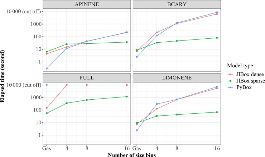
2188                 L. Huang and D. Topping: JlBox v1.1: a Julia-based multi-phase atmospheric chemistry box model

cesses and compounds, however, likewise requires us to ex-         Box in comparison with other models whilst presenting a
pand our aerosol modelling frameworks to capture this in-          narrative on required future developments. We present JlBox
creased complexity. It also raises an important question about     as a platform for a range of future developments, including
the appropriate design of community-driven process mod-            the addition of internal/external aerosol processes currently
els that can adapt to such increases in complexity, and also       not captured. It is our hope that the demonstration of Julia-
about how we ensure our platforms exploit emerging compu-          specific functionality in this study will facilitate this process.
tational platforms, if appropriate.
   In this paper we present a new community atmospheric 0D
box model, JlBox, written in Julia. Whilst the first version of    2   Model description
JlBox, v1.1, has the same structure and automatic model gen-
                                                                   The gas-phase reaction of chemicals in atmosphere follows
eration approach as PyBox (Topping et al., 2018), we present
                                                                   the gas kinetics equation:
significant improvements in a number of areas. Julia is a rel-
atively new programming language, created with the under-          d           X                   Y
standing that “Scientific computing has traditionally required        [Ci ] = − rj Sij , rj = kj        [Ci ]Sij ,                    (1)
                                                                   dt          j                 ∀i,S >0 ij
the highest performance, yet domain experts have largely
moved to slower dynamic languages for daily work” (Ju-             where [Ci ] is the concentration of compound i, rj is the re-
lia Documentation: https://julia-doc.readthedocs.io/en/latest/     action rate of reaction j , kj is the corresponding reaction rate
manual/introduction/, last access: 8 February 2021). Julia         coefficient, and Sij is the value of the stoichiometry matrix
promises computational performance close to that of For-           for compound i and j . The above ordinary differential equa-
tran, for example, without sacrificing the flexibility offered     tion (ODE), Eq. (1), fully determines the concentrations of
by languages such as Python (Perkel, 2019). In JlBox v1.1          gas-phase chemicals at any time given reaction coefficients
we evaluate the performance of a one-language-driven sim-          kj , a stoichiometry matrix {Sij } and initial values. All chem-
ulation that still utilises automated property predictions pro-    ical kinetic demonstrations in this study are provided by the
vided by UManSysProp and other informatics suites (Top-            MCM (Jenkin et al., 1997, 2002), but the parsing scheme
ping et al., 2018). The choice of programming language             allows for any mechanism provided in the standard Kinet-
when building new and sustainable model infrastructures is         ics PreProcessor (KPP) format (Damian et al., 2002). When
clearly influenced by multiple factors. These include issues       adding aerosol particles to the system, more interactions have
around training, support and computational performance to          to be considered in order to predict the state of the sys-
name a few. Python has seen a persistent increase in use           tem, including concentrations of components in the gas and
across the sciences, in part driven by the large ecosystem and     particulate phase. In JlBox v1.1 we only consider the gas–
community-driven tools that surrounds it. This was the main        aerosol partitioning to a fully moving sectional size distribu-
factor behind the creation of PyBox. Likewise, in this pa-         tion, recognising the need to use hybrid sectional methods
per we demonstrate that the growing ecosystem around Julia         when including coagulation (e.g. Kokkola et al., 2018). We
offers a number of significant computational and numerical         discuss these future developments in Sect. 5. We use bulk-
benefits to tackle known challenges in creating aerosol mod-       absorptive partitioning in v1.1 where gas-to-particle parti-
els using a one-language approach. Specifically, we make use       tioning is dictated by gas-phase abundance and equilibrium
of the ability to perform automatic differentiation of Julia       vapour pressures above ideal droplet solutions. This process
code using tools now available in that ecosystem. In JlBox         is described by the growth–diffusion equation provided by
we demonstrate the usefulness of this capability when cou-         Jacobson (2005) (pages 543, 549, 557, 560).
pling particle-phase models to a gas-phase model where de-
riving an analytical jacobian might be deemed too difficult.       d[Ci,k ]                eff             s

                                                                             = 4π Rk nk Di,k    [Ci ] − [Ci,k ] ,                     (2)
   In the following sections we describe the components in-          dt
cluded within the first version of JlBox, JlBox v1.1. In Sect. 2       s                 2mw,i
                                                                    [Ci,k ] = exp                                                     (3)
we briefly describe the theory on which JlBox is based, in-                          σ Rk ρi R∗ T
cluding the equations that define implementation of the ad-                                      [Ci,k ]                 pis R∗ T
joint sensitivity studies. In Sect. 3 we discuss the code struc-               ·                             P                    ,
                                                                                 [Ccore,k ] × core_diss + i [Ci,k ] NA
ture, including parsing algorithms for chemical mechanisms,
and the use of sparse linear solvers and pre-conditioners,               eff                     Di∗
                                                                     Di,k    =                                       ,              (4)
                                                                                            1.33Kn,i +0.71
whilst also using a range of stiff solvers included within                     1 + Kn,i         Kn,i +1    + 34 1−α
                                                                                                                 αi
                                                                                                                    i

the expanding ODE solver suite DifferentialEquations.jl. In
Sect. 4 we then demonstrate the computational performance          where [Ci,k ] is the concentration of compound i component
of JlBox relative to an existing community of gas-phase and                           s ] is the effective saturation vapour con-
                                                                   in size bin k, [Ci,k
mixed-phase box models, looking at a range of mechanisms           centration over a curvature surface of size bin k (consider-
from the Master Chemical Mechanism (MCM; Jenkin et al.,            ing Kelvin effect), Di,keff is the effective molecular diffusion

1997, 2002). In Sect. 5 we discuss the relative merits of Jl-      coefficient, Rk is the size of particles in size bin k, nk the

Geosci. Model Dev., 14, 2187–2203, 2021                                              https://doi.org/10.5194/gmd-14-2187-2021
L. Huang and D. Topping: JlBox v1.1: a Julia-based multi-phase atmospheric chemistry box model                                           2189

                                                                               dλ      ∂f (y; p)             ∂g
respective number concentration of particles, [Ccore,k ] is the                   =−             λ, λ(tF ) =    (tF )                         (6)
molar concentration of an assumed involatile core in v1.1 that                 dt         ∂y                 ∂y
may dissociate into core_diss components. For example, for                          ZtF
                                                                               ∂g       ∂f (y; p)
an ammonium sulfate core, core_diss is set to 3.0, mw,i is                        =               λ(t) dt                                     (7)
the molecular weight of condensate i, ρi is liquid-phase den-                  ∂p          ∂p
                                                                                       t0
sity, pis is pure component saturation vapour pressure, Di∗ is
the molecular diffusion coefficient, Kn,i is Knudsen’s num-                       JlBox implements the adjoint sensitivity algorithm with
ber, αi is accommodation coefficient, σ is the surface tension                 the help of an auto-generated Jacobian matrix ∂f (y; p)/∂y.
of the droplet, R∗ is the universal gas constant, NA is Avo-                   Users only need to supply the gradient function of the scalar
gadro’s number, and T is temperature.                                          function with respect to ODE states ∂g/∂y as well as the
   As we have to keep track of the concentration of every                      Jacobian function ∂f (y; p)/∂p of the RHS function with re-
compound in every size bin, this significantly increases the                   spect to parameters so as to get the sensitivity of the scalar
complexity of the ODE relative to the gas-phase model:                         function with respect to parameters ∂g/∂p at time tF . Both
                                                                               are provided automatically through the automatic differenti-
dy                                                                             ation provided by Julia.
   = f (y; p), y = (C1 , C2 , . . ., Cn ; C1,1 , C2,1 , . . ., Cn,m ),   (5)
dt

where y represents the states of the ODE, n is the number                      3    Implementation
of chemicals, m is the number of size bins, p is a vector of
parameters of the ODE, and f (y) is the RHS function implic-                   JlBox is written in pure Julia and is presently only dependent
itly defined by Eqs. (1) and (2). We extend the original ODE                   on the UManSysProp Python package for parsing chemical
state y with concentrations of each chemical on each size bin.                 structures into objects for use with fundamental property cal-
A simple schematic is provided in Fig. 1. Imagine there are                    culations during a pre-processing stage. The pre-processing
n = 800 components in the gas phase. In the configuration                      stage also includes extracting the rate function, stoichiometry
displayed in Fig. 1, the first 800 cells hold the concentration                matrix and other parameters from a file that defines the chem-
of each component in the gas phase. If our simulation has one                  ical mechanism using the common KPP format, followed by
size bin, the proceeding cells hold the concentration of each                  a solution to the self-generated ODEs using implicit ODE
component in the condensed phase. If our simulation has two                    solvers. Specifically, the model consists of six parts:
size bins, the proceeding 800 cells hold the concentration
of each component in the second size bin and so on. The                            1. Run a chemical mechanism parser.
gas-phase simulation of a mechanism with n = 800 chemi-
cals has to solve an ODE with 800 states, while the mixed-                         2. Perform rate expression formulation and optimisation.
phase simulation with m = 16 size bins will have 13 600
(= 800 + 800 × 16) states. Meanwhile, the size of the Jaco-                        3. Perform RHS function formulation.
bian matrix (required by implicit ODE solvers) will increase
                                                                                   4. Create a Jacobian of RHS function.
in a quadratic way from 800 × 800 to 13 600 × 13 600.
   Sensitivity analysis is useful when we need to investigate
                                                                                   5. Preparation and calculation for partitioning process.
how the model behaves when we perturb the model parame-
ters and initial values. One approach is to see how all the out-                   6. Adjoint sensitivity analysis where required.
puts change due to one perturbed value by simply subtracting
the original outputs from the perturbed outputs, or, in a local                   Figure 2 highlights the workflow of an implementation
sense, solving an ODE whose RHS is the partial derivative                      of JlBox, used as either a forward or adjoint model. As de-
of the respective parameter. However, this approach would                      tailed in the section on Code availability, JlBox was designed
be very expensive when we want the sensitivity of a scalar                     with both performance and ease of use in mind, where users
output with respect to all the parameters. This is often the                   can download, install and test it as a package from the Julia
case when doing data assimilation. The adjoint method can                      package manager in the command-line interface. To use the
efficiently solve the problem. Imagine there is some scalar                    model, one has to construct a configuration object containing
function g(y), and we would like to compute its sensitivity                    all the parameters and initial conditions that the model re-
against some parameters p. Introducing the adjoint vector                      quires and then supply it to JlBox’s run_simulation_*
λ(t) with the shape of g(y)’s gradient, the adjoint method                     function. The results are provided as a solution object from
could compute this in two steps (Damian et al., 2002):                         DifferentialEquation.jl providing a state vector
                                                                               at any time through interpolation (≥ 2 order), along with
  1. Solve the ODE Eq. (6) in a backward order.                                the respective name vector. Examples can be found in the
                                                                               example/ subfolder in the project repository which we re-
  2. Numerically integrate formula Eq. (7).                                    fer to in Sect. B.

https://doi.org/10.5194/gmd-14-2187-2021                                                           Geosci. Model Dev., 14, 2187–2203, 2021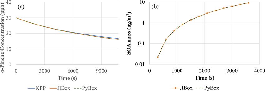
2190                   L. Huang and D. Topping: JlBox v1.1: a Julia-based multi-phase atmospheric chemistry box model

Figure 1. Array layout for ODE states y in Eq. (5).

Figure 2. Schematic illustrating the structure of JlBox v1.1, whether in forward or adjoint configuration.

3.1    Mechanism parsing and property predictions                        c C + d D represents a units of A and b units of B will
                                                                         react and produce c units of C and d units of D.
Like PyBox, JlBox builds the required equations to be solved                Upon reading each set of equations, JlBox will assign
by reading a chemical mechanism file. In the examples pro-               unique numbers for reactants and products if encountered for
vided here, we use mechanisms extracted from the Master                  the first time; then it will fill in the stoichiometry matrix Sij
Chemical Mechanism (MCM) to build the intended model                     with stoichiometry coefficients where i is the number of the
for simulation. A preview of a mechanism file is given in                equation (depicted at the beginning of each line) and j is
Listing 1.                                                               the number of the reactants and products. The stoichiome-
   There are two sections in each line of the mechanism file             try matrix is firstly built as a list of triplets (i, j, Sij ) for fast
separated by the : symbol: the first represents a single gas-            insertion of elements, and then it is transformed into the com-
phase chemical reaction where reactants before the = symbol              pressed sparse column (CSC) format, which is more memory
will react with each other with a fixed ratio and produce the            efficient for calculating the RHS of gas-kinetics.
products after the = symbol. For example, a A + b B =

Geosci. Model Dev., 14, 2187–2203, 2021                                                    https://doi.org/10.5194/gmd-14-2187-2021
L. Huang and D. Topping: JlBox v1.1: a Julia-based multi-phase atmospheric chemistry box model 2191
Listing 1. Example of the MCM file.
The latter part of a line of the chemical mechanism file,
after the symbol :, represents the expression of reaction Y
r j = kj [Ci ]Sij (8)
rate coefficient kj (y; p). The expression consists of pre-
∀i,Sij >0
scribed combinations of basic arithmetic operators + - *
/ **, basic math functions, photolysis coefficients J(1), Following this, the model calculates the rate of change
. . . , J(61), ambient parameters and intermediate variables (loss/gain) of reactants and products in each equation and
which have explicit expressions determined by the chemi- sums the loss/gain of the same species across different equa-
cal mechanism. The drawback of this approach is that pre- tions using the following:
processing is separated from simulation, and automatic code d X
generation could, in theory, introduce errors that are hard [Ci ] = − rj Sij . (9)
dt j
to debug. However, such a drawback is avoided in JlBox
with the help of Julia’s meta-programming, which assem- There are two ways to implement this. The first projects
bles the function for calculating reaction rate coefficients the structure to program instructions executed by the RHS
“on the fly”. Since the abstract representation of the func- function. The second stores it as data and the RHS function
tion is in the tree format, JlBox also does constant fold- loops through the data to calculate the result.
ing optimisation to the function where expressions are re- The first method is intended to statically figure out the
placed by their evaluated values if all of the values inside symbolic expressions of the loss and gain for each species as
the expressions are found to be constants. For example, the combinations of rate coefficients and gas concentrations, and
expression 1.2*EXP(1000/TEMP) will be replaced by to generate the RHS function line by line from the relevant
34.340931863060504 given a constant temperature at expressions. This method is straightforward and fast, espe-
298.15 K. To further reduce computation, when a reaction cially for small cases. However, it consumes lots of memory
rate coefficient is constant, the related expression is deleted and time for compiling when the mechanism file is large (i.e.
from the function which is called at every time step to up- > 1000 equations).
date the coefficients, and the respective initial value of the The other approach is to use spare matrix manipulation
coefficient is set to be the constant. because of the sparse structure of the stoichiometry ma-
The gas–aerosol partitioning process requires additional trix in atmospheric chemical mechanisms. Considering equa-
pre-processing of several parameters of each compound re- tion numbers as columns, compounds numbers as rows and
quired by the growth equation. These are listed in Eqs. (2) to signed stoichiometry (positive for products and negative for
(4). Python packages UManSysProp (Topping et al., 2018) reactants) as values, most columns of the stoichiometry ma-
and OpenBabel (O’Boyle et al., 2011) are called during the trix have limited (usually ≤ 4) nonzero values because most
pre-processing stage to calculate thermodynamic properties equations have a limited number of reactants and products.
required by those parameters. Therefore, the accumulated rate of change of each compound
can be expressed as a sparse matrix–vector product of the
3.2 Gas kinetics and gas–aerosol partitioning process stoichiometry matrix and the rates of equations vector while
the rates of equations vector can be calculated by loops with
When solving the ODE, the RHS function of the gas-phase
cached indices. This method has comparable speed to the
kinetics firstly updates the non-constant rate coefficients
previous one and consumes much less memory when com-
kj (y; p) and then constructs the reaction rate rj from concen-
piling and running.
trations of compounds [Ci ], their stoichiometry matrix (Sij ),
The gas–aerosol partitioning component of JlBox simu-
and rate coefficients kj .
lates the condensational growth of aerosols in discrete size
https://doi.org/10.5194/gmd-14-2187-2021 Geosci. Model Dev., 14, 2187–2203, 20212192 L. Huang and D. Topping: JlBox v1.1: a Julia-based multi-phase atmospheric chemistry box model
bins where each particle has the same size. Please note that backward differentiation formula (BDF) types of solvers
as we use a fully moving distribution in v1.1, when we fur- as our problem is numerically stiff. Most of the available
ther refer to a size bin we retain a discrete representation with solvers are adaptive meaning that they would choose every
no defined limits per bin. time step in an adaptive sense to achieve some absolute
and relative errors given by the user. Higher error tolerance
4 allows larger time steps, resulting in faster simulation time
π nk ρk Rk3 = mk (10)
3 X and vice versa. The error tolerance could also influence
mk = mcore,k + mi,k the convergence of fully implicit ODE solvers due to the
i non-linear nature of the ODE, so it may fail to converge if
mw.i [Ci,k ] the tolerance is too high. Note that native Julia ODE solvers
mi,k =
NA in the OrdinaryDiffEq.jl sub-package make use of
X mi,k
!−1 the parallel (dense) linear solver while the CVODE_BDF
mcore,k solver in Sundials.jl sub-package does not. This could
ρk = +
i
mk ρi mk ρcore mean that the native TRBDF2 solver could be faster than
CVODE_BDF on multiprocessor machines, although they
JlBox computes the rate of loss/gain for gas-phase and adopt similar algorithms. This would need to be profiled
condensed-phase substances through all size bins. Firstly, for across a range of examples.
each size bin k, the corresponding concentrations of each Since all the states in the ODE (Eqs. 1, 2) represent the at-
compound in the condensed phase {[Ci,k ]|∀i} are summed. mospheric abundance of compounds in each phase, it is im-
Then the model calculates all the values required by the RHS portant to preserve the non-negativeness of those states. This
of Eq. (2). As we adopted the moving bin scheme in v1.1, can be ensured by rejecting any states with negative figures
it keeps track of the bin sizes Rk as they grow during the and shrinking the time step. Users can specify whether to en-
process following formulas Eq. (10) where for each size bin able it in the configure object, and it is only available in native
k, mk denotes mass of all the particles, mi,k denotes con- Julia solvers in the OrdinarDiffEq.jl subpackage.
densed mass of compound i, mcore,k denotes the mass of in- The Jacobian matrix of the RHS ∂f (y; p)/∂y is needed in
organic core of the particles, and ρcore denotes the density of implicit ODE solvers as well as in adjoint sensitivity analy-
inorganic core. Finally, the rate of change of a given species sis. The accuracy of the Jacobian matrix, however, has vari-
d[Ci,k ]/dt is summed across all bins to give the correspond- able requirements in each case. For implicit ODE solvers,
ing loss/gain of gas-phase concentrations according to con- when doing forward simulations, the accuracy of the matrix
servation law. only affects the rate of convergence instead of the accuracy of
d X Xd the result. Some methods like BDF and Rosenbrock–Wanner,
[Ci ] = − rj Sij − [Ci,k ] (11) by design, could tolerate inaccurate Jacobian matrices (Wan-
dt j k
dt
ner and Hairer, 1996, p114). Meanwhile, for adjoint sensi-
The combination of the gas-phase Eq. (9) and condensed- tivity analysis, accurate Jacobian matrices are needed as they
phase Eq. (11) rate of change expressions provides the over- explicitly appear in the RHS function of Eq. (6).
all RHS function Eq. (5) of a multi-phase. JlBox implements an analytical Jacobian function for both
Please note we explicitly simulate the partitioning of wa- gas kinetics and the partitioning process as well as those
ter between the gaseous and condensed phase following ev- generated using finite differentiation and automatic differ-
ery other condensate. We appreciate this may significantly entiation. Theoretically, an analytical Jacobian is the most
reduce the run-time of the box model. However, in this in- accurate and efficient approach but can be laborious to im-
stance we wish to retain the explicit nature of the partition- plement due to the nature of the equations involved and
ing process before applying any simplifications, as we briefly therefore error-prone due to manual imputation. The finite-
discuss in Sect. 5.2 difference approximation can have low numerical accuracy
and high-performance costs due to multiple evaluations of
3.3 Numerical methods and automatic differentiation the RHS function, although it is the simplest to implement
and is applicable to most functions. Automatic differentiation
JlBox uses the DifferentialEquations.jl shares the advantages of both methods mentioned previously;
library to solve the ODE, assembling the it has the convenience of automatically generating a Jaco-
RHS function in a canonical way: function bian matrix from the Julia-based model, much like the finite-
dydt!(dydt::Array{L. Huang and D. Topping: JlBox v1.1: a Julia-based multi-phase atmospheric chemistry box model 2193
must be fully written in the Julia language, and this dictates stitution that sometimes needs to be updated to retain prox-
any additional work that might be required. JlBox uses the imity with the changing Jacobian.
ForwardDiff.jl library to perform auto-differentiation. In JlBox, the functions for solving P−1 x = b and updat-
The library introduces the dual-number trick with the help of ing P are specified by “prec” and “psetup” arguments in-
Julia’s multiple dispatch mechanism. side the CVODE_BDF solver. JlBox provides default prec
To improve performance and reduce memory consump- and psetup as a tri-diagonal pre-conditioner following
tion, JlBox has special treatments for computing the Ja- the approach used in AtChem (Sommariva et al., 2020). In
cobian of mixed-phase RHS. Firstly, the gas kinetic part psetup, a full Jacobian is calculated in sparse format fol-
∂fi /∂yj |1≤i,j ≤n is produced analytically because it is sparse lowed by taking its tridiagonal values forming the approxi-
and has simple analytical form, while auto-differentiation mated tridiagonal M. A LU factorisation is then calculated
tools will waste lots of memory and time as they treat it as using the Thomas algorithm and stored in a cache so that
a dense matrix. Secondly, according to Eq. (11), one part of prec can solve the linear equation quickly.
the Jacobian could be expressed as the sum of another part:
3.5 Adjoint sensitivity analysis
∂fi
1≤i≤n,n+1≤j ≤n+nm (12)
∂yj In this section we demonstrate the ability to build and de-
ploy an adjoint model. Using it to quantify sensitivity typ-
!
∂ X d
= − yk ically relies on experimental data and processes that will
∂yj dt
ni+1≤k≤(n+1)i be incorporated in future versions. Nonetheless, the exam-
X ∂fk ple given in Sect. 4.2 demonstrates the ability to evaluate
= − , the sensitivity of predicted secondary organic aerosol to all
ni+1≤k≤(n+1)i
∂yj
gas-phase kinetic coefficients. An adjoint sensitivity analysis
which could also reduce computation. We only have to com- computes the derivatives of a scalar function g(y) of the ODE
pute the Jacobian of Eq. (2) using methods mentioned previ- states with respect to some parameters p of the RHS func-
ously. For comparison of performance and accuracy, JlBox tion f (y; p). The actual computation reformulates solving
implements two auto-differentiated Jacobians for aerosol the ODE Eq. (6) in a backward order and numerically inte-
processes called “coarse_seeding” and “fine_seeding” with grating formula Eq. (7). It is worth noting that the equation is
and without the optimisations mentioned above. According in the linear form, so using an implicit method that linearises
to benchmark results presented in Appendix Table B1, it was the RHS function like the Rosenbrock method may give a
found those optimisations could significantly reduce memory good result. The Rosenbrock method explicitly includes the
usage without effecting the performance. Jacobian function as an estimation of the RHS function. In
this case, such an estimation is an exact representation which
3.4 Sparse linear solvers and pre-conditioners enables longer time steps. The BDF may also benefit from
this for the same reason, with the number of Newton steps
As the size of the Jacobian matrices grow quickly (O(n2 )) reduced to one or two. As the Jacobian matrix is frequently
following the growth of number of states n, it becomes in- called, a fast and accurate Jacobian function is needed. With
creasingly slow when simulating a multi-phase model on the this in mind, the special treatment of automatic differenti-
full MCM which has 47 544 states when using 16 size bins. ation mentioned in Sect. 3.3 delivered a 10× improvement
The majority of time is spent in solving the dense linear equa- in performance compared with the one that simply wraps the
tion Mx = b where M = I − γ J, J is the Jacobian matrix, γ RHS with the AD function. For the second step, we adopt the
is a scalar set by ODE solver, and x and b are some vectors. adaptive Gauss–Kronrod quadrature to calculate the formula
Following the Kinetic PreProcessor (KPP) and AtChem accurately.
model approach (Sommariva et al., 2020; Damian et al., Solving the ODE Eq. (6) in a backward manner poses a
2002), as the Jacobian is quite sparse JlBox introduces significant problem as we need to evaluate (an accurate) Ja-
the option to use sparse linear solvers provided by cobian matrix in a backward order (from tF to t0 ) which re-
DifferentialEquations.jl. Specifically JlBox is quires accessing the states y(t) at given time points in back-
optimised for the iterative sparse linear solver GMRES in ward order. The only way to achieve that is to store a se-
CVODE_BDF by providing pre-conditioners which could ries of states yi at some checkpoints ti . The stored states
drastically reduce the number of iterations of iterative sparse alone are sufficient for using ODE solvers with a fixed time
linear solvers like GMRES. Theoretically, a pre-conditioner step, but an adaptive ODE solver is needed for better er-
P is a rough approximation of the matrix M so that P−1 M has ror control which requires accessing y(t) at an arbitrary
less condition number than M. It is “rough” in the sense that time t. Thus we need to interpolate those states into dense
the pre-condition process of solving P−1 x = b is easier. In outputs. Since the time derivative of y is easily accessible
practice, the pre-conditioner P is stored in lower–upper (LU) in the form of dy/dt = f (y), we can use Hermite inter-
factored form so that solving P−1 x = b is a simple back sub- polation or higher order interpolation to enhance the accu-
https://doi.org/10.5194/gmd-14-2187-2021 Geosci. Model Dev., 14, 2187–2203, 20212194 L. Huang and D. Topping: JlBox v1.1: a Julia-based multi-phase atmospheric chemistry box model
racy of the interpolation. JlBox utilises the solution object Table 1. Initial conditions and solver configurations.
of DifferentialEquations.jl (which internally im-
plements Hermite interpolation) to provide y(t) at any given Mechanism α-Pinene subset of MCM
point t0 ≤ t ≤ tF . Initial condition 18 ppm ozone, 30 ppm α-pinene
Start time 12:00 GMT (noon)
Temperature 288.15 K
4 Model output
Simulation Gas phase only Mixed phase
The goal of JlBox is to provide a high-performance mech- Relative humidity Ignored 50 %
anistic atmospheric aerosol box model that also retains the Simulation period 10 800 s 3600 s
flexibility and usability of Python implementations, for ex- No. of states 305 2801 (305 + 16 × 156)
ample. Not only should it have comparable performance, Absolute tolerance 10−3 10−2
if not run faster, than other models for a given scenario, it Relative tolerance 10−6 10−4
should have the capacity for integrating benchmark chemi-
cal mechanisms with coupled aerosol process descriptions.
In this section we validate the output of JlBox against PyBox PyBox and KPP are performed on a PC with a CPU of 8-core
since the model process representations are identical, whilst AMD Ryzen 1700X at 3.6 GHz and 16 GB RAM.
also investigating the relative performance as the “size” of Figure 3 clearly shows that JlBox and PyBox produced
the problem scales. identical results, as designed. Although very close, there is
around 1 % deviation between the KPP-generated model and
4.1 Verification against existing box models the other two models. A possible explanation includes dif-
ferences between ODE solvers as JlBox and PyBox used
To test the numerical correctness of JlBox, we ran our model CVODE while KPP used LSODEs. For mixed-phase simu-
together with existing box model including PyBox and KPP lations, JlBox and PyBox again generate identical values for
with identical scenarios. JlBox is designed as a more efficient secondary organic aerosol mass, as expected.
version of PyBox, so it is expected to have identical results
in both gas- and mixed-phase scenarios. Meanwhile, gas- 4.2 Evaluation of adjoint sensitivity analysis
phase models constructed from the widely used KPP soft-
ware could provide some guarantee that the results from Jl- A demonstration of an adjoint sensitivity analysis is con-
Box is useful. However, aerosol processes are not available ducted to calculate the partial derivative of secondary organic
in KPP; as a result we could only compare outputs of gas aerosol (SOA) mass at the end of the simulation with re-
kinetics. We prepared two test scenarios with gas-phase sim- spect to the rate coefficients of each equation in the mech-
ulation only and multi-phase simulation. The settings of the anism. The configurations of the simulation are the same as
simulations are listed in Table 1. Additionally, in the multi- the mixed-phase α-pinene scenario (Table 1) presented in the
phase simulation, we set the initial aerosol to be an ideal previous section.
representation of an ammonium sulfate solution satisfying a The results presented in Table 2 highlighted the top 10 (in
lognormal size distribution with an average geometric mean terms of absolute magnitude) estimated deviations of SOA
diameter of 0.2 micrometres and a standard deviation of 2.2, mass dSOA under a 1 % change of rate coefficients because
discretised into 16 bins. The bins are linearly separated in the derivate itself (dSOA/dratecoeff) is not comparable due
log-space where a fixed volume ratio between bins defines to different units involved. The reactions between α-pinene
the centre of the bin and bin width. The upper and lower and ozone have the most substantial effect. The order of the
size range and required number of bins define the centre (ra- equations simply highlights the flow of α-pinene to its sub-
dius) of each bin accordingly. The saturation vapour pressure sequent products. This could be attributed to the fact that the
threshold of whether to include the gas-to-particle partition- system has not reached the equilibrium state (also illustrated
ing of a specific chemical is chosen to be 10−6 atm based in the growth of SOA mass in Fig. 3). Another interesting
on an extremely low absorptive partitioning coefficient for a point is that competing reactions have similar sensitivities
wide range of pre-existing mass loadings. For all simulations but opposite signs to the reactions of APINOOB, APINOOA,
presented in this paper we use the vapour pressure technique and APINENE + OH. The competing reactions between α-
of Joback and Reid (1987). Whilst known to systematically pinene and ozone is an outlier with a ratio of 5 between the
under predict saturation vapour pressures for species of at- two. A plausible explanation is that for those reactions with
mospheric interest (Bilde et al., 2015), we use it for illustra- opposite sensitivities, the products of one leads to little or
tive purposes here, and any of the methods included within no SOA while the other contributes more, so when the for-
UManSysProp can be called within JlBox. For gas-phase- mer reaction is accelerated due to its perturbed rate coeffi-
only simulations, we use α-pinene as an indicative VOC cient, it reduces the ability of the latter reaction to produce
degradation scheme. The simulations to compare JlBox with SOA. As a result, the two reactions have opposite sensitiv-
Geosci. Model Dev., 14, 2187–2203, 2021 https://doi.org/10.5194/gmd-14-2187-2021L. Huang and D. Topping: JlBox v1.1: a Julia-based multi-phase atmospheric chemistry box model 2195
Figure 3. Comparison of gas-only (a) and multi-phase (b) simulation.
ities. For the reactions of APINENE and O3, it is possible and 7 GB memory each to exploit parallelism between differ-
that the APINOOA and APINOOB pathways both produce ent initial conditions. This was chosen as a PC would have to
SOA, and the first produces more than the second one. When run them in sequential order making it too time consuming.
the rate coefficient of the second reaction is increased, the The elapsed time taken by JlBox is plotted in Fig. 4. The
decrease in SOA due to less APINOOA does not offset the average time is around 7 h which is approximately 1/10 of
increase in SOA due to more APINOOB, which leads to a simulation time. In addition, the maximum memory con-
smaller but still positive sensitivity of SOA. As we state ear- sumption is 8216 MB and average consumption is 4273 MB.
lier, a deeper analysis with alternative options for saturation This represents a significant reduction when compared to
vapour pressures and process inclusion may reveal important the memory required to store a Jacobian matrix in a dense
dependencies. double-precision format. Note that the Euler cluster pro-
vides three types of CPU nodes equipped with Intel XeonE3
4.3 Performance on large-scale problems 1585Lv5, XeonGold 6150 and AMD EPYC 7742 and the
simulation jobs are distributed to all three kinds of node.
In this section we demonstrate the performance of JlBox Although XeonE3 has better single-core performance com-
on “large-scale” problems where both KPP and PyBox fail pared to the other two, the time variations between different
to solve due to constraints imposed by the model work- scenarios far exceeds the variations due to the difference in
flow and language dependencies as shown in Appendix B. processors.
We define “large-scale” problems as those beyond single Figure 5 shows the generation of SOA mass in the 72 h
VOCs or gas-phase-only simulations. Equipped with a sparse period. JlBox captures a diurnal change of photolysis rate as
linear solver and auto-generated tridiagonal preconditioner, is depicted in experiment A. We remind the reader that we
JlBox is ideal for simulating larger mechanisms than we have no depositional loss, or variable emissions, and that we
present above. With this in mind, the largest possible mecha- are using the boiling point method of Joback and Reid (1987)
nism accessible from the MCM suite is selected, which con- for estimating saturation vapour pressures. We also present a
tains 16 701 chemical equations and 5832 species. Moreover, time series plot (Fig. 6) for experiment A1 with the high-
we performed 72 h mixed-phase simulations with 16 mov- RH scenario. Small size bins went through condensational
ing bins. This means that JlBox has to solve a system of growths within this first few hours as expected from the gas–
stiff ODEs of 47 544 variables that requires solving matrices aerosol partitioning process.
of 47 544 × 47 544 at each time step. The initial conditions
are taken from an existing representative chamber study on
mixed VOC systems (Couvidat et al., 2018, Tables 1 and 2) 5 Discussion
(see Appendix A) with 16 experiments in two sets. We use
average values of temperature where ranges are provided. 5.1 Comparison with other models
In addition, instead of using the relative humidity selected
in those studies, we performed perturbed simulations with JlBox is developed based on the PyBox model (Topping
a low-relative-humidity (RH) scenario (10 %) and high-RH et al., 2018): they have similar structures, rely on the same
scenario (80 %) respectively to investigate possible depen- methods for calculating pure component properties and pro-
dence on stiffness according to variable partitioning from the vide almost identical results. Despite these similarities, we
gas to the condensed phase. All the simulations were exe- feel JlBox has made significant improvements over PyBox in
cuted on the ETH Zurich Euler cluster, requesting 4 cores terms of readability, functionality, scalability and efficiency
https://doi.org/10.5194/gmd-14-2187-2021 Geosci. Model Dev., 14, 2187–2203, 20212196 L. Huang and D. Topping: JlBox v1.1: a Julia-based multi-phase atmospheric chemistry box model
Table 2. Sensitivities of SOA mass with respect to gas-phase rate coefficients. The units of the last two columns depend on the number of
reactants.
Reaction dSOA (µg m−3 ) dSOA/dratecoeff Rate coeff.
APINENE + O3 = APINOOA 0.157379287 3.003 × 10¹⁷ 5.240 × 10⁻¹⁷
APINENE + O3 = APINOOB 0.032264464 9.236 × 10¹⁶ 3.493 × 10⁻¹⁷
APINOOB = C96 O2 + OH + CO 0.006269052 1.254 × 10⁻⁶ 5.000 × 10⁵
APINOOB = APINBOO −0.00626905 −1.254 × 10⁻⁶ 5.000 × 10⁵
APINOOA = C109 O2 + OH 0.005857979 1.302 × 10⁻⁶ 4.500 × 10⁵
APINOOA = C107 O2 + OH −0.00585798 −1.065 × 10⁻⁶ 5.500 × 10⁵
C107O2 = C107 OH 0.005301915 −1.257 × 10² 4.218 × 10⁻³
APINENE + OH = APINBO2 0.005155068 2.643 × 10¹⁰ 1.950 × 10⁻¹¹
APINAO2 = APINBOH 0.005082219 8.207 × 10² 6.192 × 10⁻⁴
APINENE + OH = APINCO2 −0.00460746 −1.112 × 10¹¹ 4.144 × 10⁻¹²
Figure 4. Elapsed time of 72 h mixed-phase simulations. The initial conditions used for each case are listed in Appendix A.
from both a programming and algorithmic sense (Table 3). to build the adjoint model of a fully coupled process model
The Julia programming language makes the most signifi- which explicitly requires the Jacobian matrix for the entire
cant contribution to those improvements in that it promises model, let alone to extend the model with more processes.
a high-performance environment, close to Fortran, without Besides, the adaptation of sparse matrices for gas kinetics
sacrificing the flexibility of Python. For example, the directly reduced the compilation cost to a small constant value en-
translated partitioning code in JlBox can run at a compara- abling the JlBox to simulate large-scale mechanisms such as
ble speed to the individual Fortran routines in PyBox, and the entire MCM, which for PyBox typically remains limited
the multiple dispatching mechanism makes it trivial for im- by memory.
plementing the automatic differentiation. As a result, JlBox Compared to other models like KPP (Damian et al., 2002)
elegantly solves the “two-language problem” without com- and AtChem (Sommariva et al., 2020), JlBox is unique due
promising anything by writing everything in Julia. It spares to its ability to perform coupled mixed-phase simulation ef-
users from editing “code in code” like PyBox and makes it ficiently, especially on large mechanisms such as the full
easier to maintain the code base and to extend the model. MCM where the vanilla KPP variant often fails to compile.
The homogeneous code base of JlBox also enables a conve- JlBox is written in pure standard Julia without any string ma-
nient migration to other devices like GPUs considering there nipulation to codes, in contrast to KPP and AtChem, which
is already a GPU backend for Julia. enables full IDE support making it more developer friendly.
As for algorithmic advances, the automatic differentiation
method for generating Jacobian matrices is not only the most 5.2 Future development
effective addition but also a fundamental one. It is an accurate
and convenient way to calculate the Jacobian matrix which
There are a number of processes and algorithmic implemen-
only requires an RHS function fully written in Julia. With Ja-
tations not included in this version of JlBox that would be
cobian matrices available, the number of RHS evaluations is
useful for further use in a scientific capacity. These include
dramatically reduced since the implicit ODE solver no longer
coagulation, hybrid sectional methods and auto-oxidation
needs to estimate the Jacobian matrix using finite differences.
products schemes to name a few (Ehn et al., 2014; Hallquist
Also, without automatic differentiation, it will not be so easy
et al., 2009; Riemer et al., 2009). As we state earlier, the
Geosci. Model Dev., 14, 2187–2203, 2021 https://doi.org/10.5194/gmd-14-2187-2021L. Huang and D. Topping: JlBox v1.1: a Julia-based multi-phase atmospheric chemistry box model 2197
Figure 5. Time series plot of SOA mass from the same case studies used in profiling total simulation time. In this study, as noted in the
text, we use a predictive technique that under-predicts the saturation vapour pressure to create the maximum number of viable condensing
products.
Table 3. Comparison between JlBox and PyBox.
PyBox JlBox Advantage of JlBox
Language Python and Numba or Fortran Pure Julia Less code, easier to maintain
and extend
Parallelization OpenMP Parallel Linear Solver N/A
Code generation Printing string Meta-programming: generating Free syntax check, less human
the abstract syntax tree (AST) error, easier to maintain
Gas kinetics Static code generation Sparse matrix manipulation Much less compiling time,
much less memory consump-
tion
Property calculation Python code calling Translated Julia code calling N/A
UManSysprop UManSysprop (Python library)
Partitioning Fortran code Translated Julia code Simpler automatic differentia-
tion
RHS function Python code calling Julia code Faster, less memory consump-
Fortran/Numba tion
ODE solver CVODE_BDF CVODE_BDF or native solvers More selections and faster
Sparse Jacobian N/A Support with GMRES linear Enable large-scale mixed-phase
solver simulation
Jacobian matrix Handwritten Fortran code for Handwritten/automatic differ- Less human error, much eas-
gas kinetics entiated/finite differentiated ier to extend the model, faster
Jacobian for gas kinetics and mixed-phase simulation, en-
partitioning, automatic/finite abling local sensitivity analysis
differentiation can be applied based on a Jacobian
to any additional modules
Sensitivity analysis N/A Adjoint sensitivity analysis Adjoint sensitivity analysis
purpose of this development stage was to create and pro- could, and will, provide options for implementing simplified
file the first Julia implementation of an aerosol box model approaches to aerosol process, such as operator splitting, and
for the scientific community that would demonstrably ex- assume instantaneous equilibration for water in a range of
ploit the exciting potential this emerging language has to sub-saturated humid conditions. Indeed, these methods have
offer. In version 1.0 we provide a fully coupled model. We proven to provide robust mechanisms for mitigating compu-
https://doi.org/10.5194/gmd-14-2187-2021 Geosci. Model Dev., 14, 2187–2203, 20212198 L. Huang and D. Topping: JlBox v1.1: a Julia-based multi-phase atmospheric chemistry box model Figure 6. Time series plot of size bins for experiment A1 with the high-RH scenario. tational efficiency barriers if implemented correctly. How- ever, our ethos with JlBox is to build and develop a plat- form for a benchmark community box model that exploits the aforementioned benefits that Julia provides. This includes the ability to exploit existing and emerging hardware and software platforms as we try to tackle the growing chem- ical and process complexity associated with aerosol evolu- tion. We hope that, with version 1.0, the community can help develop and expand this new framework. Quantifying the importance, or not, of process and chem- ical complexity requires a multifaceted approach. With the proliferation of data-science-driven approaches across most scientific domains, Reichstein et al. (2019) note that the next generation of earth system models are likely to merge ma- chine learning (ML) and traditional process-driven models to attempt to solve the aforementioned challenges in com- plexity whilst exploiting the rich and growing datasets of global observations. Julia is being used in the development of ML frameworks, with libraries such as Flux-ML enabling researchers to embed process-driven models within the back propagation pipeline (Innes, 2018). This opens up the possi- bility to develop observation-driven parameterisations in hy- brid mechanistic-ML frameworks, which helps with the issue around provenance in ML parameterisation developments. JlBox will continually grow and we encourage uptake and further developments. Geosci. Model Dev., 14, 2187–2203, 2021 https://doi.org/10.5194/gmd-14-2187-2021
L. Huang and D. Topping: JlBox v1.1: a Julia-based multi-phase atmospheric chemistry box model 2199
Appendix A: Initial condition of Sect. 4.3
Table A1. Initial condition for anthropogenic VOC experiments from Couvidat et al. (2018). Concentrations in ppb, temperature (T ) in
Kelvin and relative humidity in %.
Experiment Toluene o-Xylene TMB Octane NO NO2 HONO T RH
A1 102 22 153 85 19 0 99 299–305 10–16
A2 200 49 300 155 23 0 75 302–305 9–18
A3 48 11 106 42 23 0 71 302–307 6–14
A4 98 24 160 79 37 0 156 297–307 6–13
A5 97 21 146 81 4 8 52 297–308 7–14
A6 93 22 146 78 21 0 94 300–308 0.4
A7 107 26 160 89 21 0 89 306–309 7–10
A8 116 29 19 10 57 0 119 302–305 15–18
A9 81 21 118 65 31 0 90 299–303 28–37
Table A2. Initial condition for biogenic VOC experiments from Couvidat et al. (2018). Concentrations in ppb, temperature (T ) in Kelvin and
relative humidity in %.
Experiment Isoprene α-Pinene Limonene NO NO2 HONO SO2 T RH
B1 107 66 58 34 128 99 0 302–307 0.5–3
B2 92 50 50 48 0 87 0 298–300 30–26
B3 122 71 40 41 0 53 0 297–300 19–22
B4 0 63 65 32 0 101 0 294–298 8–13
B5 99 59 53 150 0 307 0 295–297 8–11
B6 87 50 51 244 89 40 513 295–300 15–19
B7 55 79 76 198 0 165 461 302–305 20–30
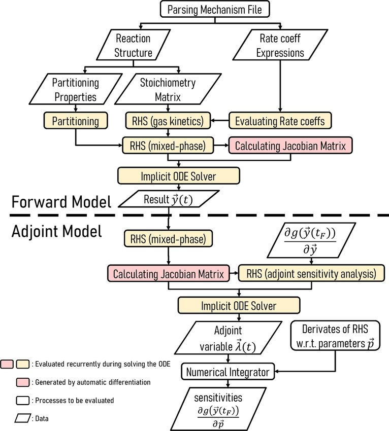
https://doi.org/10.5194/gmd-14-2187-2021 Geosci. Model Dev., 14, 2187–2203, 20212200 L. Huang and D. Topping: JlBox v1.1: a Julia-based multi-phase atmospheric chemistry box model Appendix B: Performance benchmarking In Table B1, we measured the elapsed time and total allo- cated memory of simulations using varying ODE solvers and techniques of computing the Jacobian matrix mentioned in Sect. 3.3. We chose two ODE solvers: CVODE_BDF and TRBDF2. CVODE_BDF is part of the Sundials suite devel- oped by Lawrence Livermore National Laboratory. It is a widely used high-performance ODE solver suitable for large- scale stiff ODE problems. TRBDF2 is a Julia-native library implemented in OrdinaryDiffEq.jl. It uses the clas- sical TRBDF2 scheme (Hosea and Shampine, 1996) while benefiting from a high-performance linear solver provided by the Julia community. In Table B2 the elapsed time of PyBox, JlBox and KPP are measured, with initial conditions and parameters in Sects. 4.1 and 4.2. We fine tuned JlBox on its ODE solver options to achieve the best performance. For the APINENE mechanism, CVODE with dense Jacobian was found to be the fastest on the gas-phase-only simulations, CVODE with sparse Jaco- bian was fastest for the multi-phase simulation, while the Julia-native TRBDF2 solver runs better on the adjoint sen- sitivity analysis. For the full MCM, due to memory restric- tions, the only practical option is to use the CVODE ODE solver with the FGMRES sparse linear solver. As shown in Fig. 6, we conducted simulations with vary- ing size bins and mechanism complexity to further illustrate the scaling property of JlBox compared with PyBox. We built simulations around two additional mechanisms that represent beta-caryophyllene and limonene (referred to using identi- fiers BCARY and LIMONENE respectively), which are sub- sets of the full MCM. The configurations of simulations are set to be identical to those provided in Table 1. The results in Table B2 and Fig. 6 show that the sparse multi-phase JlBox (referred to as “JlBox sparse”) performs much better than PyBox, especially for large simulations, because the perfor- mance reliance on using a sparse Jacobian scales roughly linearly with the number of size bins.The same is not true when using a dense Jacobian within JlBox (referred to as “Jl- Box dense”). For gas-phase-only simulations, interestingly the simulation overhead of JlBox is larger than PyBox for simulations of a single VOC but outperforms PyBox when simulating the entire MCM. Indeed, in this scenario, PyBox ran out of memory in our simulations. Geosci. Model Dev., 14, 2187–2203, 2021 https://doi.org/10.5194/gmd-14-2187-2021
L. Huang and D. Topping: JlBox v1.1: a Julia-based multi-phase atmospheric chemistry box model                                  2201

Table B1. Elapsed time and total allocated memory of the multi-phase APINENE simulation in Sect. 4.1 with different ODE solvers and
Jacobian matrix evaluation techniques.

                                                       Elapsed time (seconds)/total allocated memory
                                  Jacobian type            TRBDF2                          CVODE
                                  Fine seeding         38.8/2.82 GB                    340/1.30 GB
                                  Coarse seeding       40.3/8.62 GB                    350/14.8 GB
                                  Fine analytical      35.8/2.66 GB                    390/1.43 GB
                                  Coarse analytical    40.5/2.58 GB                    357/721 MB
                                  Finite difference    48.4/13.1 GB                    393/25.5 GB

Table B2. Performance comparison of PyBox, JlBox and KPP based on elapsed time of forward and adjoint simulation in Sects. 4.1 and 4.2
and simulation of full MCM with the same initial condition.

                                                                       Elapsed time (seconds)
                      Mechanism, simulation type             PyBox     JlBox   JlBox adjoint                KPP
                      APINENE, gas only                          0.3     4.5           N/A                    0.5
                      APINENE, mixed phase                      230       37             45                  N/A
                      Full MCM, gas only              out of memory       60           N/A      failed to compile
                      Full MCM, mixed phase           out of memory    1199        > 10 000                  N/A

Figure B1. Performance comparison between JlBox and PyBox with different numbers of size bins and mechanisms.

https://doi.org/10.5194/gmd-14-2187-2021                                                 Geosci. Model Dev., 14, 2187–2203, 2021
2202 L. Huang and D. Topping: JlBox v1.1: a Julia-based multi-phase atmospheric chemistry box model
Code availability. The exact code for JlBox v1.1 used in this paper Review statement. This paper was edited by Sylwester Arabas and
can be found on Zenodo at https://doi.org/10.5281/zenodo.4519192 reviewed by two anonymous referees.
(Huang, 2021a). The generated KPP α-pinene model can be found
at https://doi.org/10.5281/zenodo.4075632 (Huang, 2020). The Jl-
Box project GitHub page can be found at https://github.com/
huanglangwen/JlBox (Huang, 2021b). We also provide scripts for References
building Docker containers to build and run the exact versions
of PyBox (v1.0.1), KPP (v2.1) and JlBox (v1.1) to reproduce Amundson, N. R., Caboussat, A., He, J. W., Martynenko, A. V.,
results provided in this paper. This includes the use of Uman- Savarin, V. B., Seinfeld, J. H., and Yoo, K. Y.: A new inor-
SysProp (v1.01) and OpenBabel (v2.4.1). Those scripts can be ganic atmospheric aerosol phase equilibrium model (UHAERO),
found at https://github.com/huanglangwen/reproduce_model (last Atmos. Chem. Phys., 6, 975–992, https://doi.org/10.5194/acp-6-
access: 8 February 2021), with instructions on how replicate 975-2006, 2006.
the simulations conducted in this paper. The full specification Bilde, M., Barsanti, K., Booth, M., Cappa, C. D., Donahue, N. M.,
of dependencies of JlBox used in this paper can be found in Emanuelsson, E. U., McFiggans, G., Krieger, U. K., Marcolli, C.,
jlbox\manifest_details.txt in that repository. An archived copy of Topping, D., Ziemann, P., Barley, M., Clegg, S., Dennis-Smither,
the same repository and information can be found on Zenodo at B., Hallquist, M., Hallquist, Å. M., Khlystov, A., Kulmala, M.,
https://doi.org/10.5281/zenodo.4543713 (Huang, 2021c). JlBox is Mogensen, D., Percival, C. J., Pope, F., Reid, J. P., Ribeiro Da
an open-source model, licensed under a GPL v3.0. It has been de- Silva, M. A., Rosenoern, T., Salo, K., Soonsin, V. P., Yli-Juuti,
veloped to ensure compatibility with Julia v1, Sundials.jl and Ordi- T., Prisle, N. L., Pagels, J., Rarey, J., Zardini, A. A., and Riip-
naryDiffEq.jl where detailed dependency information is available inen, I.: Saturation Vapor Pressures and Transition Enthalpies
in the reproduction repository. As noted on the project GitHub of Low-Volatility Organic Molecules of Atmospheric Relevance:
page, JlBox can also be installed through the Julia package man- From Dicarboxylic Acids to Complex Mixtures, Chem. Rev.,
ager which deals with all required dependencies. The PyBox project 115, 4115–4156, https://doi.org/10.1021/cr5005502, 2015.
page can be found at https://doi.org/10.5281/zenodo.1345005 Couvidat, F., Vivanco, M. G., and Bessagnet, B.: Simulating
(Topping, 2021) (https://github.com/loftytopping/PyBox, last ac- secondary organic aerosol from anthropogenic and biogenic
cess: 8 February 2021). PyBox is an open-source model, li- precursors: comparison to outdoor chamber experiments, ef-
censed under GPL v3.0. The KPP project page can be found fect of oligomerization on SOA formation and reactive up-
at http://people.cs.vt.edu/asandu/Software/Kpp/ (last access: 16 take of aldehydes, Atmos. Chem. Phys., 18, 15743–15766,
February 2021). KPP is an open-source project, licensed un- https://doi.org/10.5194/acp-18-15743-2018, 2018.
der GPL v2.0. The UmanSysProp project page can be found Damian, V., Sandu, A., Damian, M., Potra, F., and Carmichael,
at https://doi.org/10.5281/zenodo.4110145 (Shelley and Topping, G. R.: The kinetic preprocessor KPP - A software environ-
2021) (https://github.com/loftytopping/UmanSysProp_public, last ment for solving chemical kinetics, Computers and Chemi-
access: 8 February 2021). UManSysProp is an open-source project, cal Engineering, 26, 1567–1579, https://doi.org/10.1016/S0098-
licensed under GPL v3.0. 1354(02)00128-X, 2002.
Ehn, M., Thornton, J. A., Kleist, E., Sipilä, M., Junninen, H.,
Pullinen, I., Springer, M., Rubach, F., Tillmann, R., Lee, B.,
Author contributions. JlBox was written and evaluated by LH. DT Lopez-Hilfiker, F., Andres, S., Acir, I. H., Rissanen, M., Joki-
provided guidance on comparisons with PyBox, including mapping nen, T., Schobesberger, S., Kangasluoma, J., Kontkanen, J.,
the same structure to JlBox, and helped in the effective design and Nieminen, T., Kurtén, T., Nielsen, L. B., Jørgensen, S., Kjaer-
sustainability of JlBox. gaard, H. G., Canagaratna, M., Maso, M. D., Berndt, T., Petäjä,
T., Wahner, A., Kerminen, V. M., Kulmala, M., Worsnop,
D. R., Wildt, J., and Mentel, T. F.: A large source of low-
volatility secondary organic aerosol, Nature, 506, 476–479,
Competing interests. The authors declare that they have no conflict
https://doi.org/10.1038/nature13032, 2014.
of interest.
Hallquist, M., Wenger, J. C., Baltensperger, U., Rudich, Y., Simp-
son, D., Claeys, M., Dommen, J., Donahue, N. M., George, C.,
Goldstein, A. H., Hamilton, J. F., Herrmann, H., Hoffmann, T.,
Acknowledgements. This work was supported by the EPSRC Iinuma, Y., Jang, M., Jenkin, M. E., Jimenez, J. L., Kiendler-
UKCRIC Manchester Urban Observatory (University of Manch- Scharr, A., Maenhaut, W., McFiggans, G., Mentel, T. F., Monod,
ester) (grant number: EP/P016782/1). The authors would like to ac- A., Prévôt, A. S. H., Seinfeld, J. H., Surratt, J. D., Szmigiel-
knowledge the assistance given by Research IT at the University of ski, R., and Wildt, J.: The formation, properties and impact of
Manchester. The authors would also like to acknowledge the ETH secondary organic aerosol: current and emerging issues, Atmos.
Zurich Euler cluster for supporting large-scale simulations. Chem. Phys., 9, 5155–5236, https://doi.org/10.5194/acp-9-5155-
2009, 2009.
Hosea, M. and Shampine, L.: Analysis and implementation of
Financial support. This research has been supported by the En- TR-BDF2, in: Method of Lines for Time-Dependent Problems,
gineering and Physical Sciences Research Council (grant no. Appl. Numer. Math., 20, 21–37, https://doi.org/10.1016/0168-
EP/P016782/1). 9274(95)00115-8, 1996.
Huang, L.: KPP archived generated schema for APINENE v0.1,
Zenodo, https://doi.org/10.5281/zenodo.4075632, 2020.
Geosci. Model Dev., 14, 2187–2203, 2021 https://doi.org/10.5194/gmd-14-2187-2021You can also read