SUIHTER: A new mathematical model for COVID-19. Application - arXiv.org
←
→
Page content transcription
If your browser does not render page correctly, please read the page content below
SUIHTER: A new mathematical model for COVID-19. Application
                                                 to the analysis of the second epidemic outbreak in Italy
                                                 Nicola Parolini1 , Luca Dede’1 , Paola F. Antonietti1 , Giovanni Ardenghi1 , Andrea
                                                 Manzoni1 , Edie Miglio1 , Andrea Pugliese2 , Marco Verani1 , and Alfio Quarteroni1,3
                                                          1
arXiv:2101.03369v2 [q-bio.PE] 12 Jan 2021

                                                            MOX, Department of Mathematics, Politecnico di Milano, Italy
                                                              2
                                                                Department of Mathematics, University of Trento, Italy
                                            3
                                              Institute of Mathematics, École Polytechnique Fédérale de Lausanne (EPFL), Switzerland
                                                                                (Professor Emeritus)

                                                                                       January 13, 2021

                                                                                            Abstract
                                                     The COVID-19 epidemic is the last of a long list of pandemics that have affected humankind
                                                 in the last century. In this paper, we propose a novel mathematical epidemiological model named
                                                 SUIHTER from the names of the seven compartments that it comprises: susceptible uninfected
                                                 individuals (S), undetected (both asymptomatic and symptomatic) infected (U), isolated (I),
                                                 hospitalized (H), threatened (T), extinct (E), and recovered (R). A suitable parameter calibra-
                                                 tion that is based on the combined use of least squares method and Markov Chain Monte Carlo
                                                 (MCMC) method is proposed with the aim of reproducing the past history of the epidemic in
                                                 Italy, surfaced in late February and still ongoing to date, and of validating SUIHTER in terms of
                                                 its predicting capabilities. A distinctive feature of the new model is that it allows a one-to-one
                                                 calibration strategy between the model compartments and the data that are daily made avail-
                                                 able from the Italian Civil Protection. The new model is then applied to the analysis of the
                                                 Italian epidemic with emphasis on the second outbreak emerged in Fall 2020. In particular, we
                                                 show that the epidemiological model SUIHTER can be suitably used in a predictive manner to
                                                 perform scenario analysis at national level.

                                            1    Introduction
                                            The Coronavirus pandemic of coronavirus disease 2019 (COVID-19) is a tremendous threat to
                                            global health. Since the outbreak in early December 2019 in China, more than 1 834 573 global
                                            deaths have been registered, while the estimated total number of confirmed cases is 84 511 153 up to
                                            January 2nd, 2020 [1]. The real number of people infected is unknown, but probably much higher.
                                                In this scenario, predicting the trend of the epidemic is of paramount importance to mitigate
                                            the pressure on the health systems and activate control strategies (e.g. quarantines, lock-downs,
                                            and suspension of travel) aiming at containing the disease and delaying the spread.
                                                As these predictions have vital consequences on the different actions taken from governments
                                            to limit and control the COVID-19 pandemic, the recent period has seen considerable flowering
                                            of epidemiological mathematical models; see, e.g, [6, 13, 19, 20, 26, 32]. However, estimates and

                                                                                                 1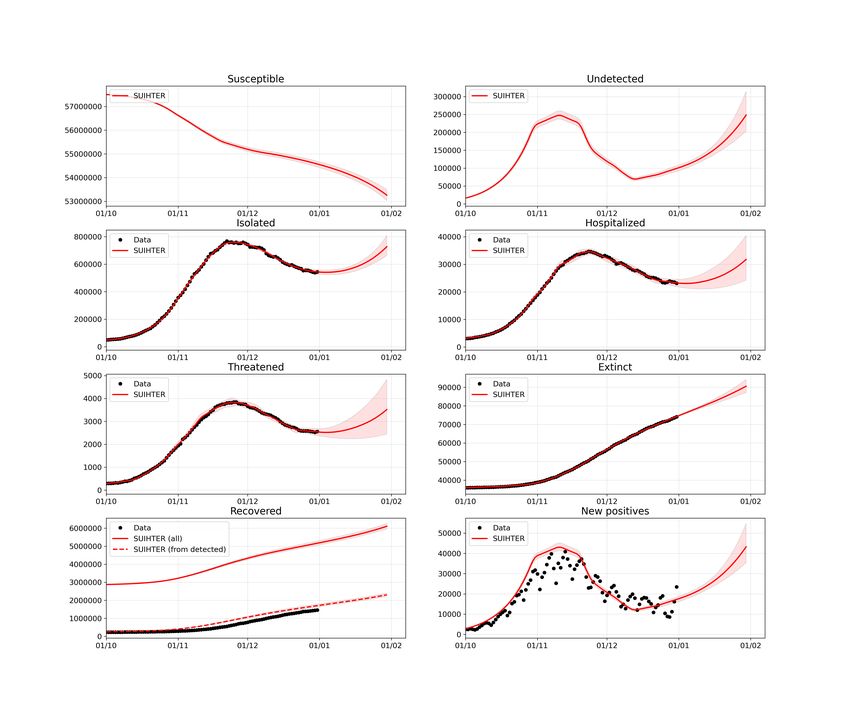
scenarios emerging from modeling highly depend on different factors, ranging from epidemiological
assumptions to, perhaps most importantly, the completeness and quality of the data based on
which models are calibrated. Since the beginning of the COVID-19 emergency, the quality of data
on infections, deaths, tests, and other factors have been spoiled by under-detection or inconsistent
detection of cases, reporting delays, and poor documentation. This inconvenient has affected, and
still is to date hampering, the intrinsic predictive capability of mathematical models.
     Despite the lack or incompleteness of the available data, which makes modeling the current
COVID-19 outbreak challenging, mathematical models are still vital to establish predictions within
reasonable ranges, and can be adapted to incorporate the effects of public health authority in-
terventions in order to estimate in advance their effectiveness and their impact on the COVID-19
spread. Building upon the celebrated SIR (susceptible (S), infectious (I), and recovered (R)) model
proposed in 1927 by Kermack and McKendrick [22], several generalizations have been formulated
over the years by enriching the number of compartments, e.g. Susceptible – Exposed – Infectious
– Recovered (SEIR), Susceptible - Infectious - Susceptible (SIS), Susceptible - Exposed - Infected
- Recovered - Deceased (SEIRD), Susceptible – Exposed – Infectious – Asymptomatic – Recovered
(SEIAR), Susceptible - Infectious - Susceptible - Recovered (SIRS), Susceptible - Exposed - Infec-
tious - Quarantined - Recovered (SEIQR), Maternally - derived immunity - Susceptible – Exposed
– Infectious – Recovered (MSEIR), ... ; we refer to, e.g., [7, 21, 28] for an overview. Overall, these
models have been abundantly applied to locally analyze COVID-19 outbreak dynamics in various
countries (see, e.g., [23, 25, 26, 27]).
     However, the peculiar epidemiological traits of the COVID-19 ask for models better able to
accurately portray the mutable dynamic characteristics of the ongoing epidemic, with particular
emphasis on two critical aspects: (i) the crucial rôle played by the undetected (both asymptomatic
and symptomatic) individuals; (ii) the number of individuals that require Intensive Care Unit
(ICU) admission . This latter aspect is of paramount importance in designing realistic scenarios
that incorporate the pressure of the epidemic on the national health systems.
     In this paper we introduce a new mathematical model, named SUIHTER, based on the initials
of the seven compartments that it comprises: susceptible uninfected individuals (S), undetected
(both asymptomatic and symptomatic) infected (U), isolated (I), hospitalized (H), threatened (T),
extinct (E), recovered (R). It is a system of coupled ordinary differential equations (ODEs) that
are driven by a set of parameters that are indeed piecewise constant time dependent functions.
A first set of parameters denote the transmission rates due to contacts between susceptible and
undetected, quarantined or hospitalized subjects. A second set of parameters mimics the rates
at which I (isolated) and H (hospitalized) individuals develop clinically relevant or life-threatening
symptoms. A further parameter indicates the probability rate of detection of previously undetected
infected individuals. Another set of parameters indicates the rate of recovery for the four classes
of infected subjects. Finally, a last parameter denotes the mortality rate.
     This new model has been conceived to face some of the limitations that can be found in exist-
ing epidemiological models applied to the COVID-19 pandemic. On the one hand, some studies
adopt simple SIR-like models [23, 26, 27], which have the advantage of having a limited number of
parameters to be calibrated, but pay the price of being unable to track the dynamics of different
categories of infected individuals. On the other hand, the sophisticated multi-compartmental mod-
els (see e.g. [6, 20]) have been proposed to account for the state-of-the-art knowledge of the clinical
characterization for different classes of infected individuals according to the actual level of disease
severity. However, it is not always possible (and, even when possible, it is not easy) to associate

                                                  2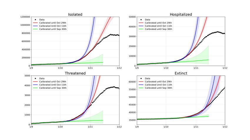
the multiple infected compartments to the available data. The SUIHTER model has been designed
with the objective of creating the most compact model able to predict the different categories of
infectious individuals which are considered relevant by the policy makers. The model adopts a
two-step calibration process based on a preliminary estimation of the model parameters that uses a
Least Squares minimization, followed by a Bayesian calibration performed through a Markov Chain
Monte Carlo algorithm. The model has been adopted to simulate the second COVID-19 epidemic
outbreak in Italy arisen in Fall 2020 (and still ongoing). In particular, we have investigated the
capability of the model in forecasting with an adequate advance notice the activation of exponential
growth at the beginning of a new outbreak, as well as the occurrence of a peak for the most relevant
compartments. Results of the calibration, simulation by SUIHTER and predictions for few Italian
regions, namely Lombardy, Emilia-Romagna and Lazio, are also reported.
    The outline of the paper is as follows: in Section 2 we introduce the SUIHTER mathematical
model; Section 3 is devoted to the description of the calibration procedure, Section 4 contains the
numerical results along with their discussion. In Section 5, we draw our conclusions and we discuss
some model’s limitations.

2    Mathematical model
The spread of COVID-19 had made it clear that it is of paramount importance to include in
epidemiological models a compartment describing the dynamics of infected individuals that are
still undetected. This is, e.g., the case of [20]. However, some compartments presented in [20]
(undetected asymptomatic infected and undetected symptomatic infected) are virtually impossible
to be validated since these classes of individuals cannot be traced in public databases (cf. [2]). For
this reason, building upon [20] we propose a new model more suited to taking full advantage of
publicly available data. In particular, our model is described by the following system of ordinary
differential equations

                                    βU U (t) + βI I (t) + βH H (t)
                    Ṡ (t) = −S (t)                                ,
                                                   N
                                   βU U (t) + βI I (t) + βH H (t)
                    U̇ (t) = S (t)                                − (δ + ρU ) U (t) ,
                                                 N
                    I˙ (t) = δU (t) − (ρI + ωI +γI ) I (t) +θH H (t),
                                                                                                  (1)
                    Ḣ (t) = ωI I (t) − (ρH + ωH +θH +γH )H(t)+θT T (t),

                    Ṫ (t) = ωH H (t) − (ρT + θT + γT ) T (t) ,

                    Ė (t) = γI I (t)+γH H (t)+γT T (t) ,

                    Ṙ (t) = ρU U (t) + ρI I (t) + ρH H (t) + ρT T (t)

where the compartments of the model are defined as follows (see Figure 1):

    • S: number of susceptible (uninfected) individuals;

    • U : number of undetected (both asymptomatic and symptomatic) infected individuals;

    • I: number of isolated (quarantined) individuals;

                                                   3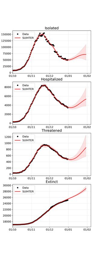
Figure 1: Interactions among compartments in SUIHTER model

   • H: number of hospitalized individuals, respectively;

   • T : number of threatened (acutely symptomatic infected, detected) individuals;

   • E: number of extinct individuals;

   • R: number of recovered individuals,

and N = S + U + I + H + T + E + R denotes the total population (assumed constant).
    The model is characterized by the following 15 parameters, some of which are possibly chosen
as time dependent piece-wise polynomial functions:

   • βU , βI , βH denote the transmission rates due to contacts between a susceptible subject and
     an undetected infected, a quarantined, or a hospitalized subject, respectively;

   • ωI denotes the rate at which I-individuals develop clinically relevant symptoms, while ωH
     denotes the rate at which H-individuals develop life-threatening symptoms;

   • θH and θT denote the rates at which H and T -individuals improve their health conditions
     and return to the less critical I and H compartments, respectively;

   • δ denotes the probability rate of detection, relative to undetected infected individuals;

   • ρU , ρI , ρH and ρT denote the rate of recovery for the four classes of infected subjects;

                                                 4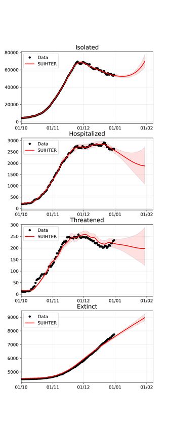
• γI , γH and γT denote the mortality rates for the individuals isolated at home, hospitalized
      and hosted in ICUs, respectively.

    In mathematical epidemiology a fundamental quantity is the basic reproduction number (denoted
by R0 ), which is used to measure the transmission potential of a disease. It represents the average
number of secondary infections produced by a typical case of an infection in a population where
everyone is susceptible (see [7, 28]). For our model, by using a similar argument to the one adopted
in the proof of Proposition 1 in [20], we find

                                  βU     δ βI (r3 r4 − θT ωH ) + βH ωI r4
                           R0 =        +                                     ,                   (2)
                                   r1    r1 r2 r3 r4 − r4 θH ωI − r2 θT ωH
 where r1 = δ + ρU , r2 = ρI + ωI + γI , r3 = ρH + ωH + θH + γH , and r4 = ρT + θT + γT . For the
sake of comparison (cf. Eq. (32) in [20]), we observe that in the present context the characteristic
polynomial q(s) of the Jacobian matrix associated to the linearization of (1) around the equilibrium
configuration (S̄, 0, 0, 0, 0, Ē, R̄) with S̄ + Ē + R̄ = N is

                              q(s) = s3 p(s)      with p(s) = D(s) − S̄N (s)

where

           D(s) = (s + r1 )(s + r2 )(s + r3 )(s + r4 ) − (s + r1 )θH ωI − (s + r1 )(s + r2 )θT ωH
and

N (s) = (s + r4 ){βU [(s + r2 )(s + r3 ) − ωI θH ] + βI δ(s + r3 ) + βH δωI } − βU ωH θT (s + r2 ) − βI δθT ωH .

    From the mathematical point of view, the reproduction number R0 plays the role of a threshold
value at the outset of the epidemic. If R0 > 1, the disease spreads in the population; if R0 < 1,
the number of infected gradually declines to zero. Note that all factor in Eq. (2) are, as expected,
actually positive. Furthermore, the expression (2) considerably simplifies assuming, as in the main
analysis of the paper, that θH = θT = βH = 0.
    Our SUIHTER model, as other compartmental models, corresponds to a particular case of an
integral model with arbitrary distribution of infectious time, for which R0 is well-known [14].

3     Parameter calibration
Model calibration through data fitting is essential to reproduce the past history of the epidemic
and to perform short-term forecasts by inferring the epidemiological characteristics of COVID-19.
    Here we use reported isolated, hospitalized, threatened and extinct cases data to estimate the
parameters of the proposed SUIHTER model. In particular, we perform the calibration in two
steps. Firstly, we find a set of parameter values using an (ordinary) least squares (LS) estimator.
Then, we perform a Bayesian calibration using a Markov Chain Monte Carlo (MCMC) algorithm,
starting from a prior distribution of the parameters centered about the LS estimate. Calibration
of epidemiological models has been already performed in a Bayesian framework, following the
pioneering paper by O’Neill and Roberts [31], for several infectious diseases [9, 15, 24]. In the
case of COVID-19 epidemic, Bayesian inference has been performed using simpler SIR [33, 37],
meta-community SEIR-like [6, 17, 19, 25] and SEIAR [32] models, in this latter case aiming at

                                                       5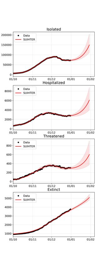
estimating nine parameters – including a dynamic, time-dependent contact rate β(t) – during the
first outbreak of the COVID-19 epidemic. In addition to model calibration, our analysis also
provides a numerical assessment of the predictive capability of the model, in forecasting with an
adequate advance notice both (i) the activation of an exponential growth at the beginning of the
outbreak, and (ii) the occurrence of a peak for the most relevant compartments.
     System (1) can be recast in the following general form describing a system of ODEs for a
state vector Y with ne components (or compartments): find Y(t) : [tI , tF ] → Rne with Y(t) =
[Y1 (t), . . . , Yne (t)]T such that

                                         Y0 (t) = F(t, Y(t); p(t)) t ∈ (tI , tF ]                                          (3)
                                         Y(tI ) = Y0 .                                                                     (4)

The evolution of the system depends on npar time-dependent parameters, collected into the function
p(t) : (tI , tF ] → Rnp . The initial conditions Y0 ∈ Rne are assumed to be known.
    Let us partition the interval I = [tI , tF ] into nph phases, corresponding to different epidemic
stages due to, e.g., partial restrictions (such as lock-down measures) or different containment rules
introduced by the Government or by the local Authorities. Moreover, assume that on each phase,
the value of the npar model parameters is constant (but unknown), so that we can introduce the
following set of admissible parameters

                         Pad = {p(t) : p(t)|Ik = pk ∈ [pL,k , pU,k ], k = 1, . . . , nph }                                 (5)

where pL,k , pU,k are given constant vectors. For the sake of notation, let us denote by p ∈ Rnp
the vectors of unknown parameters to be estimated, with np = npar nph , and let Y = Y(t, p)
highlight the dependence of the states on the parameters. Consequently, Pad is the np -dimensional
hypercube delimited by the constraints (5). Additional constraints on the parameters are assumed,
by imposing that some of them are constant on all phases.
    We consider nme measurements of ncom = 4 < ne compartments at equispaced times tj = j∆t,
j = 0, . . . , nme − 1 over the interval I = [tI , tF ], with t0 = tI , tnme −1 = tF ; in total, we have
                                                                       me −1
ncom × nme = 4 × nme reported data, say D̂(t) = {ŶI,H,T,E (tj )}nj=0        ∈ R4×nme , that is,

              ˆ 0 ), Ĥ(t0 ), T̂ (t0 ), Ê(t0 ))T , . . . , (I(t
    D̂(t) = {(I(t                                            ˆ nme −1 ), Ĥ(tnme −1 )), T̂ (tnme −1 ), Ê(tnme −1 ))T }.

   The first stage of the calibration process is then performed by seeking a LS estimate of the
parameters vector, given by the solution of the following minimization problem,

                                             p̂ = arg min {J (p)}                                                          (6)
                                                        p∈Pad

where
                                       X−1
                                      nme          X
                           J (p) :=                         αk (tj )kYk (tj , p) − Ŷk (tj )k22                            (7)
                                        j=0 k={I,H,T,E}

being Y(tj ) the solution of (3)-(4) evaluated at a certain given instant tj , j = 0, . . . , nme − 1
and k · k2 the usual Euclidean vector norm. Here, we denote by Yk , k = {I, H, T, E} the com-
ponents of the vector Y corresponding to the compartments I, H, T , and E, respectively, and by
D(t, p) = {Yk (t, p), k = {I, H, T, E}} the model outcome used for its calibration. For a balanced

                                                             6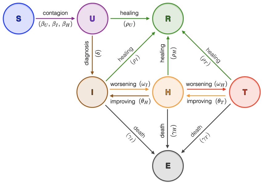
distribution of the error across the different compartments, whose amplitudes vary along time, the
dynamical weight coefficients are defined as αk (tj ) = 1/Ŷk (tj ).
    We considered the official epidemiological data supplied daily by the Italian Civil Protection,
hereafter called “raw data” and freely available at https://github.com/pcm-dpc/COVID-19, [2].
The accuracy of these data is highly questioned, in particular concerning the estimate of the total
number of infection (strongly dependent on the daily screening effort). The ncom = 4 time series
selected for model calibration (Isolated, Hospitalized, Threatened and Extincts) are those consid-
ered more reliable among the data daily supplied by the authorities. One of the key features of
the proposed SUIHTER model is indeed the one-to-one correspondence of the compartments with
the categories for which reliable data, as the ones provided on a daily-basis by the Italian Civil
Protection, are available [2].
    When nph phases are considered, equation (6) leads to the optimization of np = 15nph pa-
rameters in total. Namely, for each phase of the epidemic, we have the 15 parameters given by
[βU , βI , βH , ωI , ωH , δ, ρU , ρI , ρH , ρT , θH , θT , γI , γH , γT ].
    Unfortunately, so many parameters make the calibration process problematic. In what follows,
we calibrate our model under the following simplifying assumptions:
   • βI is taken proportional to βU , i.e. βI = αβU , α ∈ R being an additional constant parameter
     to be calibrated;
   • βH , θH , θT and γH are set to zero;
   • δ, ρU , ρI , ρH , ρT , γI ∈ R are constant on [tI , tF ].
With these restrictions, the total number of parameters to be calibrated is reduced to 4nph + 7.
    The first stage of the calibration process has been performed by solving the minimization prob-
lem (6) numerically. We have used a parallel version of the limited memory Broyden-Fletcher-
Goldfarb-Shanno algorithm with box constraints (L-BFGS-B), see [39] for details.
    The second stage of the calibration process aims at quantifying uncertainties and has been
carried out employing a Bayesian framework, since the latter provides probability densities of the
input parameters that can be propagated through the model.
    Bayesian inference allows us to construct a probability distribution function (PDF) for the
unknown parameters merging prior information and available data, these latter entering in the
expression of the likelihood function. The posterior PDF can then be obtained through the Bayes
theorem on conditional probabilities. For the case at hand, we quantify the likelihood of the
parameter vector p and model outcome D(t, p) in correlation to the reported cases D̂(t) as

                                      π(D̂(t) | p) ∼ N (D(t, p), σ 2 I)

where I ∈ R4×4 is the identity matrix and the (unknown) variance σ 2 is assumed to be constant
for each compartment.
    Using Bayes’ theorem, we obtain the posterior distribution of the parameters p accounting for
the prior knowledge on the parameters and the reported cases, as
                                        π(D̂(t) | p)π(p)             π(D̂(t) | p)π(p)
                       π(p | D̂(t)) =                      =R                             ,
                                            π(D̂(t))             P   π(D̂(t) | p)π(p)dp
where π(p) denotes the prior distribution for the parameters. Here, we assume that the prior PDF
for p is uniform, centered at the LS estimate p̂j obtained during the former calibration stage, on a

                                                       7
range [0.9p̂j , 1.1p̂j ]. An alternative, more common and rigorous procedure, would require to specify
informative priors for the parameters, starting from key epidemiological features, as done, e.g., in
[19]. However, given the large numbers of parameters to be estimated – some of which do not
find explicit counterparts in epidemiological literature – we have assumed uniform priors, centered
about the LS estimates, as a practical shortcut to overcome the difficulty in specifying the prior
distribution. In terms of predictive capability of the model, numerical results provided in Section
4 allows us to assess the proposed approach.
Since we cannot obtain the posterior distribution over the model parameters p analytically,
we adopt approximate-inference techniques based on Monte Carlo (MC) methods, which aim at
generating a sequence of random samples from a Markov chain whose distribution approaches the
posterior distribution asymptotically, whence the name of Markov chain Monte Carlo (MCMC)
[35]. In particular, we have used the delayed rejection adaptive Metropolis (DRAM) algorithm
implemented in pymcmcstat, see [29] for the details. The first 10 000 samples of the chain serve
to tune the sampler and are later discarded (burn-in period). We use the next 90 000 samples to
approximate the posterior distribution for the parameters p.
From the generated chains, we draw NM C samples of the parameters p1 , . . . , pNM C that we
use to perform forward propagation of uncertainty through the model, and to compute predictive
envelopes of the SUIHTER model compartments (or predictive distributions).
We report the MC samples of the trajectories on the time interval (tI , tf or ], including a forecast
window (tF , tf or ] that extends beyond the time window (tI , tF ] where data have been reported, to
assess the predictive capability of the model.
4 Results and discussion
In this section we present three batteries of numerical results assessing the forecasting capabilities
of the SUIHTER model. Our analysis focuses on the second wave of the epidemic that started at the
end of the Summer of 2020 and, at the time of this writing, is still affecting Italy. In Section 4.1, we
present the simulation of the second wave obtained with the SUIHTER model using for its calibration
all the data between August 20th and December 31st. By limiting the time range of the data used
for the calibration, we also investigate the model capability in forecasting the peaks of the different
compartments (see Section 4.2) and the exponential outbreak in the early phase of the second wave
(see Section 4.3).
Our results at the national level for the second outbreak have been obtained by initializing
the Isolated, Hospitalized, Threatened and Extinct compartments with the data provided by the
Dipartimento della Protezione Civile [2] at August 20th. The remaining compartments – i.e. Sus-
ceptible, Undetected and Recovered for which data are unavailable – have been instead initialized
with the values obtained by running (and calibrating) the SUIHTER model from February 24th up
to August 20th (first outbreak and its tail) with initial values set as S = 60 483 174, U = 500,
I = 94, H = 101, T = 96, E = 7 and R = 1 on February 24th. The initial values for the second
outbreak are therefore S = 57 630 019, U = 9 286, I = 15 063, H = 883, T = 68, E = 35 418 and
R = 2 793 236 on August 20th. Note that this would imply that, by the end of the first wave,
around 4.6% of the Italian population had been infected. A serosurvey organized by ISTAT and
ISS had estimated that 2.5% of the Italian population had been infected [30, 36]; the survey how-
ever had a low compliance, so that its results may be biased. A corresponding survey in Spain
[34] with a much higher compliance rate estimated seropositivity to 4.6% or 5%, depending on the
8methodology used for the seroprevalence analysis. Thus, the value obtained for August 20th looks
rather reasonable.
4.1 Simulation of the second epidemic wave
The SUIHTER model has been used to simulate the second epidemic outbreak, starting from August
20th until December 31st, 2020. The different phases in which the parameters can take different
values have been identified according to the occurrence of some critical events:
• September 24th: all schools at the national level reopened after the summer (and spring
lockdown) closure (schools calendars vary by grades and by region level in Italy);
• October 8th: new rules imposing the mandatory use of masks in all locations (either indoor
or outdoor) accessible to public;
• October 26th: confinement rules including distance learning for most secondary schools, lim-
itations on the activity of shops, bars and restaurants, strong limitation of sport and leisure
activities1 ;
• November 6th: stricter confinement rules including distance learning from 9th grade, further
restrictions on commercial activities, limitations on the circulation outside the own munici-
pality (for some Italian regions, classified as red regions)2 ;
• November 15th: additional confinement rules as more regions turned to red color 3 ;
• November 19th: additional confinement rules as more regions turned to red color4 ;
• November 29th: relaxation of confinement rules in some regions turned to orange color5 ;
• December 11th: relaxation of confinement rules in some regions turned to yellow color6 ;
• December 21st: stricter confinement rules are introduced for Christmas holidays7 .
Considering a time lag of 4 days (to account for the incubation period) [18], the corresponding
phases on which the model parameters are defined and possibly changing) are:
• Phase 1: August 20th - September 28th;
• Phase 2: September 29th - October 11th;
• Phase 3: October 12th - October 29th;
• Phase 4: October 30th - November 9th;
1
DPCM October 24, 2020, http://www.governo.it/sites/new.governo.it/files/DPCM_20201024.pdf
2
DPCM November 4, 2020, https://www.gazzettaufficiale.it/eli/gu/2020/11/04/275/so/41/sg/pdf
3
http://www.salute.gov.it/imgs/C_17_notizie_5171_0_file.pdf
4
http://www.regione.abruzzo.it/system/files/atti-presidenziali/ordinanze/2020/ordinanza-n-102.
pdf
5
http://www.salute.gov.it/imgs/C_17_notizie_5197_0_file.pdf
6
https://www.gazzettaufficiale.it/eli/id/2020/12/12/20A06975/sg
7
DPCM December 21, 2020, https://www.gazzettaufficiale.it/eli/id/2019/02/07/19A00753/sg
9• Phase 5: November 10th - November 18th;
• Phase 6: November 29th - November 23rd;
• Phase 7: November 24th - December 3rd;
• Phase 8: December 4th - December 15th;
• Phase 9: December 16th - December 25th;
• Phase 10: December 26th - December 31st.
As mentioned in Section 3, the compartments employed for calibration are only those with more
reliable data, namely Isolated (I), Hospitalized (H), Threatened (T) and Extinct (E) individuals.
We performed the model calibration by employing the MCMC parameter estimation procedure
described in Section 3, over the 10 phases using the data over the full time range between August
20th and December 31st. The simulations were run for the subsequent 30 days beyond the date
associated to the last set of data used for the calibration forecasting the evolution of the epidemic
until end of January 2021. For the new additional phase the values of the parameters are obtained
by linearly extrapolating the two (constant) values of the corresponding parameter of the last two
phases, located at the final day of each phase, namely phases 9 and 10.
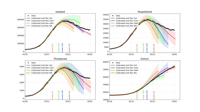
In Figure 2, we report the expected values for the time evolution of the 7 compartments of
the SUIHTER model as well as the time evolution of additional compartment of the Daily new
positive, which corresponds to δ U (t), and the corresponding 90% prediction intervals obtained by
propagating input uncertainties through the model.
We can notice that the calibrated compartments (Isolated, Hospitalized, Threatened and Ex-
tinct) fit very accurately the data time series. Two additional compartments for which data are
available but not used for the calibration, namely the Recovered and the Daily new positives, are
used to assess the accuracy of the model. In particular, since the available data for the Recovered
cases do not include the undetected cases that recovered before being detected, a novel compartment
Z t
RD (t) = (ρI I(τ ) + ρH H(τ ) + ρT T (τ )) dτ,
tI
collecting the individuals recovered after being detected is used for comparison, showing a good
match with the data. Moreover, the time history of the Daily new positives is also in reasonable
agreement with the data, proving that the model is able to capture the main dynamics of the system
also for those quantities that are not directly driven by the data calibration. Our calibration
indicates that from the rise of the second outbreak to December 31st, 2020, 4 410 025 ± 113 231
individuals have been infected, of which 66.4% ± 0.7% has been detected. In addition, the case
fatality ratio (the ratio between the total number of deceased and diagnosed individuals over the
period) is 2.6% ± 0.1%; instead, the infection fatality ratio (the ratio between the total deceased
and infected individuals, the latter either detected or undetected) to be around 1.6% ± 0.1%. This
latter figure is compatible with the infection fatality ratio estimated as 2.23% in [8] for the first
Italian outbreak. We also observe that our calculated estimates are likely to be underestimated as
the second outbreak is still ongoing at the present time and compartments of isolated and extinct
individuals become populated at different time scales.
10Figure 2: Expected values (solid lines) and 90% prediction intervals (shaded areas) for the 7
compartments of the SUIHTER model plus the additional Daily new positives compartment.
The mean values and the standard deviations computed by the MCMC calibration are reported
in Table 1 for the parameters that are constant over the simulation and in Table 2 for the param-
eters that are free to change in each phase. The former parameters and time dependent functions
represent rates that can be used to interpret the dynamics of the second Italian outbreak. For
example, large values of βU indicate sustained transmission rates at the corresponding phases. Val-
ues of healing rates ρI , ρH and ρT are proportional to the probability of healing for individuals in
the compartments I, H and T, but are inversely proportional to the corresponding average time of
healing; the rate ρI also incorporates the healing on isolated individuals who are however asymp-
tomatic. To better understand the role of the parameters, note that if they were constant, ρI ρ+ω I
I
would represent the probability for an isolated individual to recover without being hospitalized, and
11Mean Std Dev
α 0.01085 0.00059
δ 0.17420 0.00278
γI 2.43e-4 1.37e-6
ρU 0.07392 0.00274
ρI 0.03062 0.00132
ρH 0.06948 0.00226
ρT 0.07863 0.00304
Table 1: Mean values and standard deviations of the constant parameters
βU ωI ωH γT R0
Phase Mean Std Dev Mean Std Dev Mean Std Dev Mean Std Dev Mean Std Dev
1 0.26402 0.002019 0.00642 0.000317 0.01517 0.000804 0.07238 0.002805 1.119 0.0052
2 0.35072 0.003113 0.00843 0.000460 0.02251 0.001167 0.12388 0.004607 1.482 0.0144
3 0.34635 0.002448 0.00999 0.000402 0.02494 0.001156 0.09046 0.003339 1.460 0.0115
4 0.27296 0.004197 0.00753 0.000339 0.02983 0.001260 0.15781 0.002524 1.154 0.0196
5 0.24914 0.003912 0.00540 0.000264 0.02872 0.001226 0.17076 0.004714 1.058 0.0183
6 0.17528 0.004656 0.00481 0.000266 0.03088 0.001476 0.19419 0.006230 0.743 0.0219
7 0.21801 0.003305 0.00388 0.000192 0.02985 0.001292 0.19134 0.005199 0.926 0.0156
8 0.19450 0.003049 0.00370 0.000194 0.02859 0.001210 0.19086 0.004291 0.827 0.0143
9 0.26871 0.005721 0.00349 0.000183 0.02782 0.001275 0.19319 0.005484 1.143 0.0271
10 0.28086 0.004685 0.00402 0.000219 0.02889 0.001400 0.19082 0.003435 1.193 0.0222
Table 2: Mean values and standard deviations of the parameters that changes over the phases and
the corresponding R0
similarly ρHρ+ω
H
H
represents the probability for a hospitalized individual to recover without being
transferred to ICUs. In the same way, γTγ+ρ T
T
represents the probability of dying for an individual
δ
in ICUs, and δ+ρU represents the probability that an infected individual is detected.
Finally, Table 2 also reports the value of the basic reproduction number R0 calculated as in
Eq.(2) for the SUIHTER model. The calculation uses the model parameters reported in Tables 1
and 2 (columns 1 − 4). Note that the estimates of the standard deviations are strongly influenced
by the choice of the prior in the interval centered about the values obtained by the least squares
procedure ±10%. They should mainly be judged in relative terms.
We observe that the value of R0 obtained by the calibration reflects the full reopening of
educational activities and work restart after holidays, as well as the public health measures and
restrictions later introduced by authorities to contain the second epidemic outbreak. In particular,
the rise of R0 in Phases 2 and 3 follows the full schools reopening and restart of working activities
from mid September, and probably accounts for seasonality effects too. Restrictions on mobility,
schools, businesses and partial lock-downs were introduced in late October at regional and national
levels, as reflected by the decrease of R0 from Phase 4 to 6, when R0 became smaller than one.
Partial reopening and easing restrictions were gradually introduced in some regions and at the
national level from late November, as the new increment of R0 from Phase 7 indicates.
4.1.1 Simulating the second outbreak for Italian regions
The results obtained simulating the epidemic at the national scale can indeed hide specific local
outbreaks. The SUIHTER model can also simulate the evolution of the epidemic for everyone of the
12Lombardy Emilia-Romagna Lazio
Figure 3: Expected values (solid lines) and 90% prediction intervals (shaded areas) for the Isolated,
Hospitalized, Threatened and Extinct compartments in three Italian regions, from left to right
Lombardy, Emilia-Romagna and Lazio
20 Italian Regions for which the same data time series as those used for the national calibration are
available. Unfortunately, this is not true for the finer geographical level (the 107 provinces) since
only the number of total cases from the beginning of the epidemic is provided.
Following the same initialization and calibration strategies adopted for the national level, we
have carried out the simulation of the second epidemic outbreak in three Italian regions, namely
Lombardy, Emilia-Romagna and Lazio. In Figure 3, the expected value for the time evolution
of the four compartments used for the calibration and the corresponding 90% prediction intervals
are reported for the former three regions. We can observe, for instance, that: i) the peaks of
the compartments have been reached earlier in Lombardy; ii) after the peaks have been reached,
the decrease of the curves is much slower in Lazio than in the other regions. In all the cases the
results obtained by numerical simulations stand in very good agreement with the real data, with
the only exception of the threatened compartment in Lazio where a slight discrepancy (within 10%
in relative terms) is observed. Predictions realized for the former three regions indicate different
epidemic trends at the regional level.
13Figure 4: Peak forecast obtained by the SUIHTER model with different data ranges for the Isolated,
Hospitalized, Threatened and Extinct compartments
4.2 Predicting the peaks
Predicting the peak of an epidemic outbreak is a tremendous challenge for an epidemiological
model. Yet, the predictive capability of epidemiological models is of paramount importance to
inform policymakers about the dynamics of the disease and foresee timing and level of peaks of
infected, hospitalized and ICU treated individuals, as well as the potential effects of policy responses.
With the goal of investigating to which extent our SUIHTER model is able to predict the oc-
currence of the epidemic wave peak, we repeated the calibration using the data over limited time
ranges.
In particular, we have considered three different cases: in Case 0 we used all the data time
histories available until December 3rd, while in Cases 1, 2 and 3, the data employed for the
calibration were limited to November 23rd, November 19th, and November 9th, respectively. For
each case, the simulations were run for the subsequent 30 days beyond the date associated to the
last set of data used for the calibration and the linear extrapolation carried out as indicated before.
In Figure 4, we report the expected value for the time evolution of the four compartments used
for the calibration, and the 90% prediction intervals obtained by propagating input uncertainties
through the model. The accuracy of the forecast, as expected, improves as far as a richer set of
data are employed in the calibration. Our simulations show the occurrence of a peak for each of
the three compartments, not only for Case 0 in which the time lapse of the data used for the
calibration covers the peaks, but also for Case 1, 2, and 3, when the data time-series employed for
the calibration are still rising. However, we should remark that if the model is calibrated with a
14shorter time series, namely available data stop more than 30 days before the peak, the occurrence
of the peak cannot be correctly predicted.
As already noticed, because of the overall complexity of the problem and the limited data
available for its calibration, by no means we intend here to certify in rigorous terms the actual
values of the future compartments. However, in spite of the widths of the predictive intervals
(which depend, at some extent, on the widths of the chosen prior distributions), we nonetheless
observe that the expected values (solid lines in Figure 4) carry meaningful prediction capabilities.
To further quantify the prediction accuracy, it is interesting to assess this peak forecasting with
respect to the actual day and value that have been observed for the different compartments at the
end of November 2021. Moreover, we propose a comparison with the predictions obtained using the
different strategies based on data fitting recently presented in [1]. Namely, for each compartment,
we have considered both a simple polynomial (quadratic) extrapolation of their time history (a
strategy that is known to be unreliable on large time intervals), as well as a model based on the
registration of the second outbreak with the curve of the corresponding first outbreak occurred in
Spring 2020.
A comparison between the peak forecast obtained with the SUIHTER model, the quadratic ex-
trapolation (based on the last 10 days), and the registration approach is displayed in Figure 5, for
the Isolated, Hospitalized and Threatened compartments. The curves show how the prediction in
terms of day of peak occurrence and peak value changes as far as an increasing number of data are
used (the last data day is reported on the horizontal axis).
By comparing the peak predictions with the day and value of the actual measured data peak
(reported with a dashed line in Figure 5), we should first remark that the SUIHTER prediction
largely outperforms those obtained with polynomial extrapolation. Moreover, even when compared
with predictions based on the registration with the first epidemic wave, the SUIHTER model is more
accurate for most of the considered quantities. When making this comparison, it is worthy noticing
that, while prediction based on the registration strongly depends on the evolution of the different
compartment during the first epidemic wave, the predictions based on SUIHTER do not require any
a-priori knowledge of previous epidemic waves.
4.3 Predicting the outbreak
In this section we discuss the capability of the SUIHTER model of predicting the occurrence of the
exponential outbreak of the COVID-19 epidemic. To this aim, a second set of simulations have
been performed by focusing on the early stages of the second wave.
Similarly to the previous section, we have considered different calibrations based on employing
different subsets of the data available until the end of October (when the epidemic reached its
maximum rate of growth). In particular, we performed three different calibrations by employing
data until October 29th, October 11th and September 30th, respectively.
The results displayed in Figure 6, in particular the evolution of the three infected compartment,
indicate that the onset of an exponential growth activating the second wave could have been
predicted using the data available until October 11th. Also in this case, we report the expected
value for the time evolution of the 4 compartments used for the calibration, and the 90% prediction
intervals obtained by propagating input uncertainties through the model. Although in this case
the model prediction detaches from reported data at later stages – showing its extreme sensitivity
to data, typical of any exponential growth – it is remarkable that our calibration procedure would
have predicted a dramatic variation of the epidemic trend from September 30th to October 11th.
15Isolated (peak day) Isolated (peak value)
Hospitalized (peak day) Hospitalized (peak value)
Threatened (peak day) Threatened (peak value)
Figure 5: Peak day (left) and peak value (right) vs. last used data by day for the three compartments
Isolated (top), Hospitalized (middle) and Threatened (bottom), estimated with data extrapolation,
data registration and SUIHTER model
16Figure 6: Outbreak forecast obtained by the SUIHTER model with different data ranges for the
Isolated, Hospitalized, Threatened and Extinct compartments
5 Conclusions and model limitations
In this paper, we have introduced a new mathematical model, named SUIHTER, to describe the ongo-
ing pandemic of coronavirus disease 2019 (COVID-19). This epidemiological model is constructed
on seven compartments – susceptible uninfected individuals (S), undetected (both asymptomatic
and symptomatic) infected (U), isolated (I), hospitalized (H), threatened (T), extinct (E) and re-
covered (R) – and we exploit it to study and analyse the second Italian outbreak emerged in Fall
2020 and still ongoing. In particular, our model is suited for calibration against data made avail-
able daily by the Italian Civil Protection [2]. On the basis of these data at the national level,
our calibration populates the compartments I, H, T and E, which we purposely use to determine
transmission rates, rates of recovery, infection fatality rates, etc. In particular, SUIHTER is able of
determine the infected, but undetected population, a compartment (U) that is crucial for studying
and understanding the epidemic, especially considering that large shares of infected individuals
went uncounted during the first and even the second outbreaks in Italy. Moreover, thanks to our
approach transmission rates, and thus the basic reproduction number R0 , can be estimated on a
daily basis. Finally, our calibration is made robust by exploiting Bayesian estimation using the
Markov Chain Monte Carlo method.
The SUIHTER model calibrated at the Italian national level is validated against data related to
the last part of the second outbreak. Comparisons are made against basic statistical models, namely
quadratic regression and registration of the first epidemic wave. The comparison demonstrates the
better accuracy of SUIHTER for predictive purposes. This is made possible by using extrapolated
transmission rates that are calibrated at earlier times through regression models, a feature that
17allows capturing peaks of the second Italian outbreak correctly, and enables using SUIHTER in a
predictive fashion by leveraging data available at the current date. This novel approach attempts
to circumvent a common issue of the use of epidemiological compartmental models for forecasting
[32], that is accurately capturing transmission rates. However, as our approach is based on inter-
polating values of these transitions rates, the accuracy of their extrapolation and, consequently,
their exploitation for prediction within SUIHTER can only be limited to restricted time windows,
especially when government interventions and citizen behaviours are changing. Note that, although
the calibration procedure did not make any assumptions about the temporal changes in parameters,
the estimates accurately reflect the policy changes: estimates of R0 decrease as control measures
are tightened and increase when they are relaxed.
A further limitation of our approach is that we are currently calibrating the Italian epidemic
outbreaks at the national level, that is as a whole, without summing up the different contributions at
the level of the 20 Italian regions for which data are available [2]; we indeed performed the calibration
only for few of the Italian regions, namely Lombardy, Emilia-Romagna and Lazio. Populating
compartments at the national level by summing up results obtained by tailored calibrations of each
Italian region would allow a better capturing of the spatio-temporal heterogeneity of the Italian
outbreaks, which reflects different mobility patterns and density of population. In this respect,
several different approaches have been proposed in literature, see, e.g. [11] and the references
therein, ranging from the use of network based models [5, 12], to systems of ordinary differential
equations on network [3, 4], as well as non-local partial differential equations [38]. Among the
contributions appeared during the COVID-19 pandemic, we also recall the recent papers [6, 19, 25],
where a meta-community SEIR-like model has been proposed and employed to reproduce the
contagion in Italy. Still, calibrating our SUIHTER at the regional level, and for all the regions,
would require a more sophisticated design due to the intrinsic ill-posedness of the inverse problem,
especially when taking mobility patterns into account. Nevertheless, we plan to better address
spatio-temporal heterogeneity of the Italian outbreaks in the future by generalizing our SUIHTER
model to incorporate suitable spatial-multicity mobility terms at the regional level. Even if a more
spatially detailed compartment model is surely desirable, to act, for example, at the province level
(Italy is comprised of 107 provinces), at the time being no detailed data for its calibration have
been made available.
Albeit the SUIHTER is namely very sophisticated and involves 15 time-dependent parameters
and functions to be determined based on available data, we limited our calibration to a subset of
the possible control variables, by forcibly setting to zero some parameters that we deemed to be
less relevant for the transmission of the epidemic and by assuming as piece-constant over time some
other ones. We also neglected incubation tine, and we implicitly assumed that all distributions in
the states are exponential, which is far from correct [16]. Still, we believe that this qualifies as an
acceptable compromise among the complexity of the SUIHTER model and its calibration procedure,
the associated computational costs, and the accuracy of the results. Some of the calibrated param-
eters assume values that are able to compensate for those parameters prescribed a priori, even if
their interpretation may not result straightforward in explaining the outbreak. In this respect, we
plan to assess the robustness of our approach by allowing the calibration of additional parameters.
Further, our multi-compartment SUIHTER model does not consider stratification of ages groups
within the compartments. This is namely an important aspect as some compartments like H, T
and E are mostly populated by the elderly, while the transmission mechanisms widely differ by
age and context of infection (workplace, school, family, etc.). We also plan to improve SUIHTER by
18considering age stratification within its compartments.
Finally, in consideration of the ongoing emergency situation amidst the second Italian outbreak,
we believe that our SUIHTER model is well suited to be used in a predictive manner to support and
motivate public health measures. To the best of our knowledge, apart from [10] wherein a SEIRD
model is used at the regional level, SUIHTER stands as one of the first models to analyze the second
Italian COVID-19 outbreak and that can readily serve the purpose of predicting the epidemic trend.
Acknowledgements
The authors would like to thank Prof. Luca Formaggia for his insightful suggestions and careful
reading of the manuscript.
References
[1] Johns Hopkins University. COVID-19 Dashboard by the Center for Systems Science and En-
gineering, last accessed December 8, 2020. https://coronavirus.jhu.edu.
[2] Presidenza del Consiglio dei Ministri, Dipartimento della Protezione Civile, Italia, last accessed
December 8, 2020. https://github.com/pcm-dpc/COVID-19.
[3] Linda J.S. Allen, B.M. Bolker, Yuan Lou, and A.L. Nevai. Asymptotic profiles of the steady
states for an SIS epidemic patch model. SIAM Journal on Applied Mathematics, 67(5):1283–
1309, 2007.
[4] Julien Arino and P. van den Driessche. A multi-city epidemic model. Mathematical Population
Studies, 10(3):175–193, 2003.
[5] Duygu Balcan, Vittoria Colizza, Bruno Gonçalves, Hao Hu, José J. Ramasco, and Alessandro
Vespignani. Multiscale mobility networks and the spatial spreading of infectious diseases.
Proceedings of the National Academy of Sciences, 106(51):21484–21489, 2009.
[6] Enrico Bertuzzo, Lorenzo Mari, Damiano Pasetto, Stefano Miccoli, Renato Casagrandi, Marino
Gatto, and Andrea Rinaldo. The geography of COVID-19 spread in italy and implications for
the relaxation of confinement measures. medRxiv, 2020.
[7] Fred Brauer, Carlos Castillo-Chavez, and Zhilan Feng. Mathematical Models in Epidemiology.
Springer, 2019.
[8] Nicholas F. Brazeau, Robert Verity, Sara Jenks, Han Fu, Charles Whittaker, Peter Winskill,
Ilaria Dorigatti, Patrick Walker, Steven Riley, Ricardo P. Schnekenberg, Henrique Hoeltge-
baum, Thomas A. Mellan, Swapnil Mishra, H. Juliette T. Unwin, Oliver J. Watson, Zulma M.
Cucunubá, Marc Baguelin, Lilith Whittles, Samir Bhatt, Azra C. Ghani, Neil M. Ferguson, and
Lucy C. Okell. COVID-19 infection fatality ratio: estimates from seroprevalence. Technical
Report 34, Imperial College London, 2020. https://doi.org/10.25561/83545.
[9] Simon Cauchemez, Achuyt Bhattarai, Tiffany L. Marchbanks, Ryan P. Fagan, Stephen Ostroff,
Neil M. Ferguson, David Swerdlow, and the Pennsylvania H1N1 working group. Role of social
19networks in shaping disease transmission during a community outbreak of 2009 H1N1 pandemic
influenza. Proceedings of the National Academy of Sciences, 108(7):2825–2830, 2011.
[10] Giulia Cereda, Cecilia Viscardi, Luca Gherardini, Fabrizia Mealli, and Michela Baccini. A
SIRD model calibrated on deaths to investigate the second wave of the SARS-CoV-2 epidemic
in Italy. Epidemiologia & Prevenzione – Rivista dell’Associazione Italiana di Epidemiologia,
(2052), 2020.
[11] Dongmei Chen, Bernard Moulin, and Jianhong Wu. Analyzing and modeling spatial and tem-
poral dynamics of infectious diseases. John Wiley & Sons, 2014.
[12] Vittoria Colizza, Alain Barrat, Marc Barthélemy, and Alessandro Vespignani. The role of
the airline transportation network in the prediction and predictability of global epidemics.
Proceedings of the National Academy of Sciences, 103(7):2015–2020, 2006.
[13] Fabio Della Rossa, Davide Salzano, Anna Di Meglio, Francesco De Lellis, Marco Coraggio,
Carmela Calabrese, Agostino Guarino, Ricardo Cardona-Rivera, Pietro De Lellis, Davide Li-
uzza, Francesco Lo Iudice, Giovanni Russo, and Mario di Bernardo. A network model of
italy shows that intermittent regional strategies can alleviate the COVID-19 epidemic. Nature
Communications, 11(5106), 2020.
[14] Odo Diekmann and Hans J.A.P. Heesterbeek. Mathematical Epidemiology of Infectious Dis-
eases: Model Building, Analysis and Interpretation. John Wiley, 2000.
[15] Ilaria Dorigatti, Simon Cauchemez, Andrea Pugliese, and Neil Morris Ferguson. A new ap-
proach to characterising infectious disease transmission dynamics from sentinel surveillance:
Application to the Italian 2009–2010 A/H1N1 influenza pandemic. Epidemics, 4(1):9–21, 2012.
[16] Luca Ferretti, Chris Wymant, Michelle Kendall, Lele Zhao, Anel Nurtay, Lucie Abeler-Dörner,
Michael Parker, David Bonsall, and Christophe Fraser. Quantifying SARS-CoV-2 transmission
suggests epidemic control with digital contact tracing. Science, 368(6491), 2020.
[17] Seth Flaxman, Swapnil Mishra, Axel Gandy, H. Juliette T. Unwin, Thomas A. Mellan, Helen
Coupland, Charles Whittaker, Harrison Zhu, Tresnia Berah, Jeffrey W. Eaton, Mélodie Monod,
Pablo N. Perez-Guzman, Nora Schmit, Lucia Cilloni, Kylie E.C. Ainslie, Marc Baguelin, Adhi-
ratha Boonyasiri, Olivia Boyd, Lorenzo Cattarino, Laura V. Cooper, Zulma Cucunubà, Gina
Cuomo-Dannenburg, Amy Dighe, Bimandra Djaafara, Ilaria Dorigatti, Sabine L. van Elsland,
Richard G. FitzJohn, Katy A.M. Gaythorpe, Lily Geidelberg, Nicholas C. Grassly, William D.
Green, Timothy Hallett, Arran Hamlet, Wes Hinsley, Ben Jeffrey, Edward Knock, Daniel J.
Laydon, Gemma Nedjati-Gilani, Pierre Nouvellet, Kris V. Parag, Igor Siveroni, Hayley A.
Thompson, Robert Verity, Erik Volz, Caroline E. Walters, Haowei Wang, Yuanrong Wang,
Oliver J. Watson, Peter Winskill, Xiaoyue Xi, Patrick G.T. Walker, Azra C. Ghani, Christl A.
Donnelly, Steven Riley, Michaela A.C. Vollmer, Neil M. Ferguson, Lucy C. Okell, Samir Bhatt,
and Imperial College COVID-19 Response Team. Estimating the effects of non-pharmaceutical
interventions on COVID-19 in Europe. Nature, 584:257–261, 2020.
[18] Tapiwa Ganyani, Cecile Kremer, Dongxuan Chen, Andrea Torneri, Christel Faes, Jacco
Wallinga, and Niel Hens. Estimating the generation interval for COVID-19 based on symptom
onset data. MedRxiv, 2020.
20[19] Marino Gatto, Enrico Bertuzzo, Lorenzo Mari, Stefano Miccoli, Luca Carraro, Renato
Casagrandi, and Andrea Rinaldo. Spread and dynamics of the COVID-19 epidemic in Italy:
Effects of emergency containment measures. Proceedings of the National Academy of Sciences,
117(19):10484–10491, 2020.
[20] Giulia Giordano, Franco Blanchini, Raffaele Bruno, Patrizio Colaneri, Alessandro Di Filippo,
Angela Di Matteo, and Marta Colaneri. Modelling the COVID-19 epidemic and implementa-
tion of population-wide interventions in Italy. Nature Medicine, pages 1–6, 2020.
[21] Herbert W. Hethcote. The mathematics of infectious diseases. SIAM Review, 42(4):599–653,
2000.
[22] William Ogilvy Kermack and Anderson G McKendrick. A contribution to the mathematical
theory of epidemics. Proceedings of the royal society of London. Series A, Containing papers
of a mathematical and physical character, 115(772):700–721, 1927.
[23] Adam J. Kucharski, Timothy W. Russell, Charlie Diamond, Yang Liu, John Edmunds, Se-
bastian Funk, Rosalind M. Eggo, Fiona Sun, Mark Jit, James D. Munday, Nicholas Davies,
Amy Gimma, Kevin van Zandvoort, Hamish Gibbs, Joel Hellewell, Christopher I. Jarvis, Sam
Clifford, Billy J. Quilty, Nikos I. Bosse, Sam Abbott, Petra Klepac, and Stefan Flasche. Early
dynamics of transmission and control of COVID-19: a mathematical modelling study. The
Lancet Infectious Diseases, 20(5):553 – 558, 2020.
[24] Phenyo E. Lekone and Bärbel F. Finkenstädt. Statistical inference in a stochastic epidemic
SEIR model with control intervention: Ebola as a case study. Biometrics, 62(4):1170–1177,
2006.
[25] Ruiyun Li, Sen Pei, Bin Chen, Yimeng Song, Tao Zhang, Wan Yang, and Jeffrey Shaman.
Substantial undocumented infection facilitates the rapid dissemination of novel coronavirus
(SARS-CoV-2). Science, 368(6490):489–493, 2020.
[26] Elena Loli Piccolomini and Fabiana Zama. Monitoring italian COVID-19 spread by a forced
SEIRD model. PLOS ONE, 15(8):1–17, 08 2020.
[27] Benjamin F. Maier and Dirk Brockmann. Effective containment explains subexponential
growth in recent confirmed COVID-19 cases in China. Science, 368(6492):742–746, 2020.
[28] Maia Martcheva. An Introduction to Mathematical Epidemiology, volume 61. Springer, 2015.
[29] Paul R. Miles and Ralph C. Smith. Parameter estimation using the python package
pymcmcstat. In Proceedings of the 18th Python in Science Conference (SCIPY 2019), 2019.
[30] Ministero della Salute, Italy. Covid-19, the results of the seroprevalence survey illustrated,
last accessed January 8, 2020. http://www.salute.gov.it/portale/news/p3_2_1_1_1.jsp?
lingua=italiano&menu=notizie&p=dalministero&id=5012.
[31] Philip D. O’Neill and Gareth O. Roberts. Bayesian inference for partially observed stochastic
epidemics. Journal of the Royal Statistical Society: Series A (Statistics in Society), 162(1):121–
129, 1999.
21You can also read