Distinguishing the cold conveyor belt and sting jet air streams in an intense extratropical cyclone
←
→
Page content transcription
If your browser does not render page correctly, please read the page content below
Distinguishing the cold conveyor belt and
sting jet air streams in an intense
extratropical cyclone
Article

Accepted Version

Postprint

Martinez-Alvarado, O., Baker, L. H., Gray, S. L., Methven, J.
and Plant, R. S. (2014) Distinguishing the cold conveyor belt
and sting jet air streams in an intense extratropical cyclone.
Monthly Weather Review, 142 (8). pp. 2571-2595. ISSN 1520-
0493 doi: 10.1175/MWR-D-13-00348.1 Available at
http://centaur.reading.ac.uk/36256/

It is advisable to refer to the publisher’s version if you intend to cite from the
work.

To link to this article DOI: http://dx.doi.org/10.1175/MWR-D-13-00348.1

Publisher: American Meteorological Society

All outputs in CentAUR are protected by Intellectual Property Rights law,
including copyright law. Copyright and IPR is retained by the creators or other
copyright holders. Terms and conditions for use of this material are defined in
the End User Agreement .

www.reading.ac.uk/centaur

CentAUR
Central Archive at the University of Reading
Reading’s research outputs online
Distinguishing the cold conveyor belt and sting jet air
         streams in an intense extratropical cyclone
 Oscar Martı́nez-Alvarado, Laura H. Baker, Suzanne L. Gray, John Methven and R. S.
            Department of Meteorology, University of Reading, United Kingdom
                                   March 20, 2014

Correspondence to:
Oscar Martı́nez-Alvarado
Department of Meteorology, University of Reading
Earley Gate, Reading, RG6 6BB, United Kingdom
E-mail: o.martinezalvarado@reading.ac.uk
Tel: +44 (0) 118 378 5549
Fax: +44 (0) 118 378 8905

                                           1
Abstract
Strong winds equatorwards and rearwards of a cyclone core have often been associated with two
phenomena, the cold conveyor belt (CCB) jet and sting jets. Here, detailed observations of the
mesoscale structure in this region of an intense cyclone are analysed. The in-situ and dropsonde
observations were obtained during two research flights through the cyclone during the DIAMET
(DIAbatic influences on Mesoscale structures in ExTratropical storms) field campaign. A nu-
merical weather prediction model is used to link the strong wind regions with three types of
“air streams”, or coherent ensembles of trajectories: two types are identified with the CCB,
hooking around the cyclone center, while the third is identified with a sting jet, descending
from the cloud head to the west of the cyclone. Chemical tracer observations show for the first
time that the CCB and sting jet air streams are distinct air masses even when the associated
low-level wind maxima are not spatially distinct. In the model, the CCB experiences slow la-
tent heating through weak resolved ascent and convection, while the sting jet experiences weak
cooling associated with microphysics during its subsaturated descent. Diagnosis of mesoscale
instabilities in the model shows that the CCB passes through largely stable regions, while the
sting jet spends relatively long periods in locations characterized by conditional symmetric in-
stability (CSI). The relation of CSI to the observed mesoscale structure of the bent-back front
and its possible role in the cloud banding is discussed.
1 Introduction
The potential to generate strong surface winds and gusts as they pass is one of the most
important aspects of extratropical cyclones, due to the direct impact on society. The aim of
this article is to analyze the three-dimensional structure of the region of strong winds near
the center of an intense extratropical cyclone and determine the origin of air streams within
that region. The study is focused on a cyclone that developed according to the Shapiro–
Keyser conceptual model (Shapiro and Keyser, 1990). This model is characterized by four
stages of development: (I) incipient frontal cyclone, (II) frontal fracture, (III) frontal T-bone
and bent-back front, and (IV) warm-core seclusion. Frontal fracture describes the break of a
continuous thermal front as the cyclone intensifies so that the cold front is dislocated eastwards
2from the warm front with a weaker gradient in between. This region is termed the “frontal
fracture zone” and is associated with air descending cyclonically from the northwest to the
south of the frontal cyclone. The descending air gives rise to a pronounced “dry slot” in
satellite imagery. The extensive cloud wrapping around the poleward side of the cyclone core
is described as the “cloud head” (Böttger et al., 1975) and its leading extremity as the “cloud
head tip” (Browning and Roberts, 1994). Figure 1 shows a schematic diagram of the structure
of a Shapiro–Keyser cyclone during development stage III.
There are two separate regions usually associated with strong winds in Shapiro–Keyser
cyclones. The first region is the low-level jet ahead of the cold front in the warm sector of
the cyclone. This low-level jet is part of the broader air stream known as the warm conveyor
belt, which transports heat and moisture northwards and eastwards while ascending from the
boundary layer to the upper troposphere (Browning, 1971; Harrold, 1973). The second region
of strong winds develops to the southwest and south of the cyclone center as a bent-back front
wraps around the cyclone. The strong winds in this region are the focus of this contribution.
Two different air streams have been associated with strong winds in this region: the cold
conveyor belt (Carlson, 1980; Schultz, 2001) and sting jets (Browning, 2004; Clark et al., 2005).
The cold conveyor belt (CCB) is a long-lived synoptic-scale air stream on the poleward (cold)
side of the warm front that flows rearwards relative to the cyclone motion in the lower tro-
posphere. It extends round the poleward flank of the cyclone and in some mature cyclones it
wraps around the west and then equatorward flank where it provides a wind component aligned
with the system motion and therefore strong ground-relative winds. A key aspect of the CCB
is that the wind maximum is near the top of the boundary layer and slopes radially outwards
with height on the cold side of the bent-back front, as would be expected from gradient thermal
wind balance.
The term “sting jet” was introduced by Browning (2004) (see also Clark et al., 2005) to
describe strong low-level winds in the cold air between the bent-back front and the cold front
on the basis of observations of the Great October storm of 1987 from satellite, precipitation
radar and the surface wind network (Browning, 2004). The air associated with the sting jet
descends from the cloud head tip, moving ahead of it around the cyclone into the dry slot behind
the cold front. As the cyclone develops into phase III the region of weak gradients between the
3bent-back front and cold front expands and the sting jet air stream descends into this region.
Here the boundary layer has near neutral stability or potential instability (Browning, 2004;
Sinclair et al., 2010); these characteristics have been hypothesized to enhance turbulent mixing
of high momentum air down to the surface.
Clark et al. (2005) analyzed simulations of the same case using the Met Office Unified Model
(MetUM) and identified distinct clusters of trajectories calculated using model winds with sting
jet air streams. A key characteristic of sting jet trajectories is that they descend as they ac-
celerate. There are several influences on vertical motion in this sector of a cyclone. On the
largest scale, the cyclone forms as part of a baroclinic wave. On isentropic surfaces cutting
through a baroclinic wave in the mid-troposphere the generic structure of motion gives rise to
four air masses: air ascending polewards and splitting into a cyclonic and anticyclonic branch
and air descending equatorwards and also splitting into a cyclonic and anticyclonic branch
(Thorncroft et al., 1993). The two cyclonic branches wrap around the cyclone core. On higher
isentropic surfaces they are described as the cyclonic branch of the warm conveyor belt (ascend-
ing) and the dry intrusion (descending) respectively. Both the CCB (ascending or horizontal)
and sting jet air streams (descending) also turn cyclonically and are found on lower isentropic
surfaces that can intersect the ground in the warm sector. In addition to the primary circulation
of the baroclinic wave, cross-frontal circulations contribute to vertical motion. For example,
frontogenesis at the cold front contributes to ascent of the warm conveyor belt and descent of
the dry intrusion behind. Semi-geostrophic theory shows that the cross-frontal circulations are
necessary to maintain approximate thermal wind balance in a time-dependent flow and there-
fore depend on its rate of change (Hoskins and Bretherton, 1972). Schultz and Sienkiewicz
(2013) have used model diagnostics to show that descent can be enhanced in the region beyond
the cloud head tip, where the sting jet air stream descends, as a result of frontolysis. The air
stream leaves the tight gradient of the bent-back front at the west of the cyclone and therefore
the gradient must decrease with time in a Lagrangian frame. Similarly, ascent is expected in
the CCB where the bent-back front strengthens.
Several studies have investigated the mechanisms leading to sting jets. Browning (2004)
proposed that the sting jets (local wind maxima) occur beneath the descending branches of
slantwise circulations generated by the release of conditional symmetric instability (CSI) in the
4frontal fracture region between the cloud head tip and the cold front. Numerical simulations
represented some form of slantwise motion in that region (Clark et al., 2005). Analysis of model
humidity and equivalent potential temperature along trajectories indicated that the air stream
originated from a saturated region within the cloud head, but became unsaturated on descent.
This would be consistent with evaporation of cloud and banding in the cloud. A necessary
condition for CSI to give rise to slantwise convection is that the air is saturated (at least
initially). Further case studies of storms with strong winds in the sting jet region clearly identify
regions meeting the CSI criterion that also exhibit banding in the cloud head (Gray et al.,
2011). Martı́nez-Alvarado et al. (2012) used CSI diagnostics to construct a regional sting jet
climatology. They found that up to a third of a set of 100 winter North Atlantic cyclones over
the past two decades (1989-2009) satisfied conditions for sting jets (Martı́nez-Alvarado et al.,
2012). However, in other studies the importance of CSI is not as clear (Baker et al., 2013b;
Smart and Browning, 2014). In addition, there have not been detailed in-situ observations
in the appropriate region of Shapiro–Keyser type cyclones which could have established the
existence of slantwise rolls, or connection to instability with respect to CSI. Finally, Browning
(2004) and Clark et al. (2005) proposed that evaporative cooling may also enhance the descent
rate of sting jet air streams, although Baker et al. (2013b) found little impact in an idealized
cyclone simulation.
The cyclone analyzed here produced very strong winds over the United Kingdom on 8
December 2011 and was the focus of an Intensive Observing Period (IOP8) during the second
field campaign of the DIAMET (DIAbatic influences of Mesoscale structures in ExTratropical
storms) project. The storm has been the subject of extensive investigation involving not only
the present article. Baker et al. (2013a) described the flights and summarized the severe societal
impacts of the storm. Vaughan et al. (2014) give more details of the DIAMET experiment and
presents results of research on high-resolution ensemble simulations and further in-situ aircraft
observations, as well as observations from automatic weather stations across the north of the
United Kingdom. The cyclone was named Friedhelm by the Free University of Berlin’s adopt-
a-vortex scheme (http://www.met.fu-berlin.de/adopt-a-vortex/).
With its aircraft field campaigns, DIAMET joins worldwide efforts to sample weather sys-
tems through aircraft observations (e.g. Schäfler et al., 2011; Sapp et al., 2013). To the authors’
5knowledge there have only been two previous research flights into an intense cyclone of this
type, crossing the strong wind regions near the cyclone center. Shapiro and Keyser (1990)
show dropsonde sections across a similar storm observed on 16 March 1987 during the Alaskan
Storms Programme. A second cyclone that developed extremely rapidly was observed at three
stages in its evolution in IOP4 of the ERICA experiment. Neiman et al. (1993) present drop-
sonde sections through this storm and Wakimoto et al. (1992) present data from the aircraft
radar in more detail. Some common aspects of the observed structures will be compared in this
paper. Friedhelm also passed over Scotland where there is a high density automatic weather
station network and radar network estimating precipitation rate from reflectivity (discussed
by Vaughan et al. (2014)). Also, numerical models have improved considerably in the last 20
years. Here, a state of the art numerical weather prediction model is evaluated against in-situ
and dropsonde observations and then used to analyze the history of air masses passing through
the regions of strongest low-level winds. The scientific questions addressed are:
1. How are the strong-wind regions southwest of the cyclone core related to the characteristic
air streams that have been proposed to exist there (CCB and sting jet)?
2. Where trajectory analysis identifies different air streams, are they observed to have dis-
tinct air mass properties?
3. What dynamical mechanism is responsible for the observed cloud banding in the cloud
head and to the south of the cyclone?
Dropsonde and in-situ measurements are used to link the observed system to the structure
simulated in the MetUM. The model is then used to calculate the air streams and the evolution
of their properties as they move into regions of strongest winds. Throughout the paper, the
term “air stream” is identified with a coherent ensemble of trajectories that describes the path
of a particular air mass arriving in a region of strong winds. Wind speed is not a Lagrangian
tracer and typically regions of strong winds move with the cyclone and change structure as
it develops. Therefore, air flows through the strong wind regions (local wind maxima or jets)
and each air stream must be identified with the time when it is in the associated strong wind
region. Trajectory analysis is combined with potential temperature, θ, tracers to investigate
the processes responsible for the evolution of each identified air mass. Tracer observations from
6the aircraft are used to investigate whether the air streams identified are distinct in composition
or not.
The article is organized as follows. The aircraft observations, numerical model, trajectory
and tracer tools are described in Section 2. A synoptic overview of the case study and a detailed
account of the evolution of strong-wind regions near the cyclone center are given in Section 3.
In Section 4 the air masses constituting strong-wind regions are identified and classified as
CCBs or sting jets according to their evolution and properties. The conditions for mesoscale
atmospheric instabilities in the vicinity of the identified air streams are investigated in Section 5.
Finally, discussion and conclusions are given in Section 6.
2 Methodology
2.1 Available aircraft observations
Cyclone Friedhelm was observed with the instruments on board the Facility for Airborne At-
mospheric Measurements (FAAM) BAe146 research aircraft. The instruments allowed in-situ
measurements of pressure, wind components, temperature, specific humidity and total water
(all phases) as well as chemical constituents such as carbon monoxide (CO) and ozone. The
aircraft was equipped with comprehensive cloud physics instrumentation characterizing liquid
droplet and ice particle size and number distributions. A summary of the instruments, their
sampling frequency and uncertainty on output parameters is given in Vaughan et al. (2014).
The observations are shown here at 1 Hz. In addition 21 dropsondes (Vaisala AVAPS RD94)
were launched from approximately 7 km. The dropsondes contributed measurements of tem-
perature, pressure and specific humidity as a function of latitude, longitude and time (at a
sampling frequency of 2 Hz). Horizontal wind profiles were obtained by GPS tracking of the
dropsondes (logged at 4 Hz). Two sondes could be logged on the aircraft at any one time, and
the average time for sonde descent was 10 minutes, limiting the average sonde spacing to 5
minutes along the flight track or 30 km at the aircraft science speed of 100 m s−1 . The verti-
cal resolution is about 10 m. Table 1 lists the sonde release times along the three dropsonde
curtains across the cyclone.
7Table 1: Dropsonde release times
Leg 1
Dropsonde No. 1 2 3 4 5 6 7 8 9 10
Release time (UTC) 1130 1146 1158 1203 1209 1212 1217 1223 1228 1234
Leg 2
Dropsonde No. 11 12 13 14 15 16 17
Release time (UTC) 1243 1249 1255 1301 1306 1312 1318
Leg 3
Dropsonde No. 18 19 20 21
Release time (UTC) 1754 1758 1802 1806
2.2 Numerical model
The case-study has been simulated using the MetUM version 7.3. The MetUM is a finite-
difference model that solves the non-hydrostatic deep-atmosphere dynamical equations with
a semi-implicit, semi-Lagrangian integration scheme (Davies et al., 2005). It uses Arakawa C
staggering in the horizontal (Arakawa and Lamb, 1977) and is terrain-following with a hybrid-
height Charney–Phillips (Charney and Phillips, 1953) vertical coordinate. Parametrization
of physical processes includes longwave and shortwave radiation (Edwards and Slingo, 1996),
boundary layer mixing (Lock et al., 2000), cloud microphysics and large-scale precipitation
(Wilson and Ballard, 1999) and convection (Gregory and Rowntree, 1990).
The simulation has been performed on a limited-area domain corresponding to the Met
Office’s recently operational North-Atlantic–Europe (NAE) domain with 600 × 300 grid points.
The horizontal grid spacing was 0.11◦ (∼ 12 km) in both longitude and latitude on a rotated
grid centered around 52.5◦ N, 2.5◦ W. The NAE domain extends approximately from 30◦ N to
70◦ N in latitude and from 60◦ W to 40◦ E in longitude. The vertical coordinate is discretized
in 70 vertical levels with lid around 80 km. The initial and lateral boundary conditions were
given by the Met Office operational analysis valid at 0000 UTC 8 December 2011 and 3-hourly
lateral boundary conditions (LBCs) valid from 2100 UTC 7 December 2011 for 72 hours.
Several previous studies have used resolutions of this order to study this type of storm (e.g.
Clark et al., 2005; Parton et al., 2009; Martı́nez-Alvarado et al., 2010), motivated on the basis
that the fastest growing mode of slantwise instability should be resolvable at these horizontal
and vertical resolutions (Persson and Warner, 1993; Clark et al., 2005). Vaughan et al. (2014)
provide an analysis of an ensemble at 2.2-km grid spacing, including the low-level wind struc-
ture, but the domain in that case is restricted to the United Kingdom; the use of the 12-km
8grid spacing allows the simulation of a larger domain that includes the full cyclone without
dominant effects from the LBCs. Moreover, the trajectory analysis (see Sections 22.3 and 22.4)
requires a large domain to allow long trajectories to be calculated without the majority of them
leaving the domain.
2.3 Trajectory analysis
Two trajectory models are used in the paper. The first model is the Reading Offline Trajec-
tory Model (ROTRAJ) as developed by Methven (1997). Its application to aircraft flights is
detailed in Methven et al. (2003). It calculates trajectories using ECMWF (European Centre
for Medium-Range Weather Forecasts) analysis data. In this paper, the ECMWF reanalysis
dataset ERA-Interim has been used as directly output by the ECMWF model (T255L60 in hy-
brid sigma-pressure vertical coordinates every six hours). A fourth order Runge–Kutta scheme
is used for the trajectory integration (with a time-step of 15 minutes). The boundary condition
on vertical velocity is used during the interpolation to ensure that trajectories cannot intercept
the ground.
The second model, based on the LAGRANTO model of Wernli and Davies (1997), calcu-
lated trajectories using hourly output from the MetUM (in the model’s native vertical coordi-
nate). The time-stepping scheme is also fourth order Runge–Kutta. Previous comparison has
shown the LAGRANTO model and the trajectory model used here to perform similarly even
though there are differences in interpolation (Martı́nez-Alvarado et al., 2014). Atmospheric
fields, such as θ and specific humidity, were interpolated onto the parcel positions to obtain
the evolution of those fields along trajectories. The material rate of change of the fields along
trajectories was computed using a centered difference formula along the temporal axis. Thus,
rather than being interpreted as instantaneous values, rates of change along trajectories should
be interpreted as an estimate of hourly-mean values.
2.4 Potential temperature tracers
The θ-tracers used in this work have been previously described elsewhere (Martı́nez-Alvarado and Plant,
2013). They are based on tracer methods developed to study the creation and destruction of
potential vorticity (Stoelinga, 1996; Gray, 2006). Potential temperature is decomposed in a
9P
series of tracers so that θ = θ0 + P ∆θP Each tracer ∆θP accumulates the changes in θ that
can be attributed to the parametrized process P. The parametrized processes considered in this
work are (i) surface fluxes and turbulent mixing in the boundary layer, (ii) convection, (iii)
radiation and (iv) large-scale cloud and precipitation. The tracer θ0 matches θ at the initial
time. By definition, this tracer is not modified by any parametrization but it is, nevertheless,
subject to advection.
The θ-tracers and trajectory analysis provide different approximations to the Lagrangian
description of the flow field. The θ-tracers are computed on-line whereas trajectories are com-
puted off-line from hourly velocity data on the model grid. Tracer θ0 experiences transport
only, without diabatic modification. Therefore, in the absence of sub-grid mixing or numerical
advection errors (in the tracer or trajectory schemes) it is expected that θ0 conserves the same
value when sampled along a trajectory. To focus on results where the θ-tracers and trajectories
are consistent, the criterion
|θ0 (xi (tarr )) − θ0 (xi (torigin ))| < ∆θ0 .
is applied where the tolerance on non-conservation is ∆θ0 = 3.5 K. Here xi refers to a point
along trajectory i, tarr is the arrival time of the trajectory in the strong wind region (the release
time of the back trajectories) and torigin is a common reference time (0100 UTC 8 December
2011) described as the trajectory origin. Approximately 20% of trajectories are rejected by this
criterion, although the identification of air streams is insensitive to this filter.
2.5 Diagnostics to identify regions of atmospheric instability
Previous studies on sting jets have shown that the necessary conditions for conditional sym-
metric instability (CSI) are satisfied in the regions that sting jet air streams pass through
(Gray et al., 2011; Martı́nez-Alvarado et al., 2013; Baker et al., 2013b). Here we identify re-
gions that satisfy necessary conditions for instability in the analyzed case and their locations
relative to the air streams.
Conditional instability (CI) with respect to upright convection is identified in regions where
2
the moist static stability (Nm , defined as in Durran and Klemp (1982)) is negative. A necessary
condition for inertial instability (II) is that the vertical component of absolute vorticity, ζz , is
10negative. Inertial instability can be regarded as a special case of (dry) symmetric instability
(SI); in the limit that θ-surfaces are horizontal, SI reduces to II. A necessary condition for
CSI is that the saturation moist potential vorticity (MPV∗ ) is negative (Bennetts and Hoskins,
1979). MPV∗ is given by
1
MPV∗ = ζ · ∇θe∗ , (1)
ρ
where ρ is density, ζ is the absolute vorticity and θe∗ is the saturated equivalent potential
temperature. Note that θe∗ is a function of temperature and pressure, but not humidity (since
saturation is assumed in its definition). Following Schultz and Schumacher (1999) a point is
only defined as having CSI if inertial and conditional instabilities are absent. If the necessary
conditions for CI or CSI are met then they can only be released if the air is saturated, so we
apply an additional criterion on relative humidity with respect to ice: RHice > 90%. As in
Baker et al. (2013b) we use the full winds rather than geostrophic winds in these CSI and II
diagnostics. The diagnostics for the conditions for instability are applied at each grid point; a
grid point is labelled as stable (S) if none of the three instabilities are identified.
All these diagnostics indicate necessary, but not sufficient, conditions for instability. The
most basic theories for each of these instabilities rely on different assumptions regarding the
background state upon which perturbations grow, namely uniform flow for CI, uniform PV for
CSI and uniform pressure in the horizontal for inertial instability. These conditions are far from
being met in an intense cyclone where there are strong pressure gradients, wind shears and PV
gradients. Shear instability is also present on all scales and grows as a result of opposing PV
gradients in shear flows.
3 Synoptic overview and identification of regions of strong
winds
3.1 Synoptic overview
On 6 December 2011, extratropical cyclone Friedhelm started developing over Newfoundland
(50◦ N, 56◦ W). Its development was part of a baroclinic wave, in tandem with another strong
cyclone to the west (named Günther) which, as Friedhelm, reached maturity on 8 December
11Table 2: Cyclone development based on 6-hourly Met Office Analysis charts between 1200
UTC 6 December 2011 and 18UTC 9 December 2011 (archived by www.wetter3.de). The
development stage column refers to the stages in the Shapiro–Keyser model of cyclogenesis
(Shapiro and Keyser, 1990). ∆p is the pressure change in the previous 6 hours. ∆p24h is the
pressure change in the previous 24 hours.
time time latitude longitude pressure development ∆p6h ∆p24h deepening
(day) (hour) (◦ N) (◦ E) (hPa) stage (hPa) (hPa) (bergeron)
6 Dec 1200 UTC 50 -56 1019 I
1800 UTC 49 -55 1014 I -5
7 Dec 0000 UTC 51 -50 1014 I 0
0600 UTC 53 -42 1008 I -6
1200 UTC 54 -35 1001 II -7 -18 0.824
1800 UTC 55 -26 992 II -9 -22 1.007
8 Dec 0000 UTC 57 -20 977 III -15 -37 1.650
0600 UTC 58 -15 964 III -13 -44 1.927
1200 UTC 59 -7 957 IV -7 -44 1.904
1800 UTC 59 0 956 IV -1 -36 1.549
9 Dec 0000 UTC 59 2 957 IV +1 -20 0.851
0600 UTC 59 8 964 IV +7 0 0.000
1200 UTC 59 11 966 IV +2 +9 -0.379
1800 UTC 60 15 971 IV +5 +15 -0.628
2011, but near Newfoundland. Traveling to the northeast, Friedhelm continued its development
according to the Shapiro–Keyser cyclogenesis model (Shapiro and Keyser, 1990), as shown in
Table 2. The cyclone satisfied the criterion to be classified as an atmospheric ‘bomb’ by
consistently deepening by more than 1 bergeron (Sanders and Gyakum, 1980). At 1200 UTC 8
December 2011, the cyclone center was located around 59◦ N, 7◦ W, just northwest of Scotland.
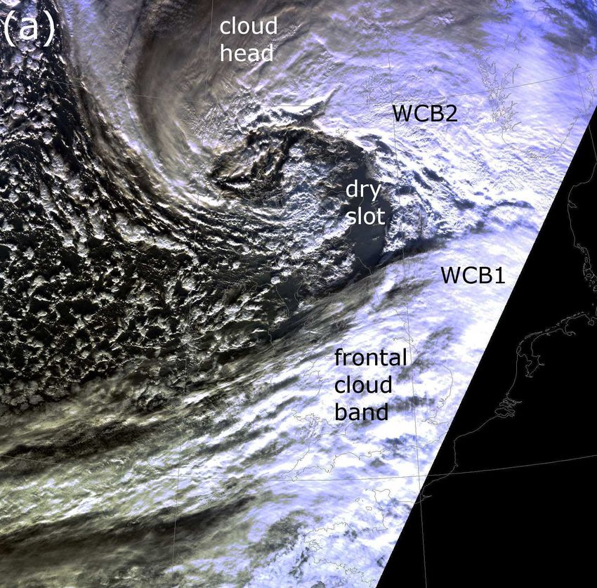
The FAAM aircraft reached the cyclone center at 1234 UTC when satellite imagery (Fig. 2a)
shows a very well-defined cloud head hooking around the cyclone center (early Stage IV). This
image also shows prominent cloud banding especially southeast of the cloud head tip, to the
southwest and south of the cyclone center.
The frontal system and the intensity of the cyclone is depicted in the Met Office analysis
valid at 1200 UTC 8 December 2011 (Fig. 2b). Figure 2c shows the synoptic situation in the
12 hour forecast using the MetUM. The similarity with the Met Office analysis chart at this
time is remarkably good in terms of the depth of the cyclone (957 hPa in both charts) and the
location of the surface fronts. The position error of the low-pressure center in the simulation is
less than 50 km.
123.2 Development of regions of strong winds
The structure of regions of strong winds to the south of the cyclone center varied throughout
the interval under study. Before 0500 UTC the only air stream associated with strong winds
was the warm conveyor belt ahead of the surface cold front (not shown). Although this region
of strong winds continued to exist throughout the interval under study, it was excluded from the
air stream analysis to focus on the strong low-level winds behind the surface cold front to the
south of the cyclone center. These winds first exceeded 40 m s−1 at 0500 UTC when a distinct
jet developed at 600 hPa. By 0600 UTC, the maximum winds (47 m s−1 ) had descended to 700
hPa. Figures 3(a–d) show the development of the ground-relative wind field on the 850-hPa
isobaric level every 3 hours from 0900 UTC to 1800 UTC. At 0900 UTC (Fig. 3a), the region of
maximum winds was about 50 km wide with winds up to 49 m s−1 spanning 600–800 hPa. By
1200 UTC (Fig. 3b), the region of maximum winds had moved over Scotland and orographic
effects might have influenced its structure. The first dropsonde curtain (D–C) crosses just to
the west of the low-level wind maximum.
By the time (1500 UTC) of the in-situ aircraft legs west of Scotland (F–G in Fig. 3c), the
wind maximum had reached the eastern side of Scotland. However, it was important for the
aircraft to remain upstream of the mountains to reduce orographic influence on the observed
winds, cloud and precipitation. The second flight dropped sondes across the low-level wind
maximum at 1800 UTC (J–H in Fig. 3d) and the subsequent in-situ legs (continuing until 2000
UTC) were at the longitude of the jet maximum but on its northern flank.
3.3 Identification of regions of strong winds
The structure of strong-wind regions, and associated temperature and humidity fields near the
cyclone center, were measured using dropsonde observations for three sections across the storm
during the two FAAM research flights (see Table 1). The dropsonde data was relayed to the GTS
(Global Transmission System) from the aircraft and was assimilated by the global forecasting
centers. All 17 sondes from the first two legs made it into the assimilation window for the 1200
UTC global analysis of both the Met Office and ECMWF, and would have influenced subsequent
operational forecasts. However, the simulation shown here starts from the global Met Office
analysis for 0000 UTC 8 December 2011 and therefore is independent of the dropsonde data.
13The first dropsonde leg (1130–1234 UTC) was from south to north towards the low-pressure
center (D–C in Fig. 3b). During this leg the aircraft flew from just north of the surface cold
front, crossing above the cloud bands into the cyclone center. Surface pressure measured by the
tenth sonde was 959 hPa, just above the minimum in the analysis at 1200 UTC. Figure 4a shows
the structure of wind speed, θe and RHice obtained from the sondes. The southern arm of the
bent-back front was crossed between 57◦ N and 57.3◦ N and divides two distinct air masses: the
cyclone’s warm seclusion to the north and the frontal fracture zone to the south. The strongest
winds are confined below 720 hPa near the bent-back front with a maximum at 866 hPa, just
above the boundary layer (51 m s−1 ). At this level, the strong winds extend southwards to
about 55.5◦ N into a region of near saturation and moist neutrality (∂θe /∂z ≈ 0). At about
56.5◦ N the strong winds extend upwards to meet the upper-level jet. Between 800 hPa and
600 hPa there is subsaturated air on the southern flank of this wind maximum and saturated
air to the north of it. In Section 4b, it will be shown that this humidity structure indicates an
air mass boundary. At 600 hPa, there is a second wind speed maximum to the south (55◦ N)
associated with the dry intrusion descending beneath the poleward flank of the upper-level jet.
It is well separated from the lower-level wind maximum discussed above and also the low-level
subsaturated air at about 56◦ N. The average sonde spacing was 30 km, but the low-level cloud
and precipitation banding (oriented perpendicular to the section) has a spacing of 25–50 km
and is therefore under-resolved by the dropsonde data. Therefore, a more fine-scale structure
in humidity cannot be ruled out.
Figure 4b shows an approximately corresponding straight section derived from model output
at 1200 UTC. In the model, the bent-back front is displaced southwards by approximately 0.2–
0.3◦ latitude (in terms of both temperature and wind). The strongest low-level winds are also
confined to a latitudinal band between 55.5◦ N and 57◦ N with nearly neutral moist stability.
However, in the model the region of strong winds extends upwards as an unbroken region
between 950 hPa and 600 hPa and the distinctive low-level maximum adjacent to the bent-
back front is missing. Moreover, the dropsonde observations reveal stronger winds near the
surface than those produced by the model between 56◦ N and 57◦ N. The moisture distribution
shows the greatest differences between observations and the model simulation. This may be
associated with the cloud bands that are too narrow to be resolved in the 12-km-grid spacing
14model. Furthermore, the model has cloud spanning the wind gradient at the bent-back front into
the warm seclusion, while the observations show saturation only to the south of the gradient.
The second dropsonde leg (1243–1318 UTC) was in a southwest direction radially away from
the cyclone center (C–E in Fig. 3b), across the cloud head tip. Figure 4c shows the structure
of wind speed, θe and RHice obtained from the dropsondes during the second dropsonde leg.
The two distinct air masses are again evident, divided by the bent-back front around 8.5◦ W
in this section. Warm seclusion air is located to the northeast, characterized by weak winds
(|V| < 20 m s−1 ) and low-level CI (below 700 hPa). The strong winds are again confined to a
band on the thermal gradient and at greater radius, in this section between 8◦ W and 9.5◦ W,
with the maximum at 859 hPa (48 m s−1 ). Note that θe and wind speed contours are aligned
and slope radially outwards with altitude (above 850 hPa). This structure was observed on
several sections across the ERICA IOP4 case (Neiman et al., 1993). Thorpe and Clough (1991)
pointed out that where the absolute momentum and saturated θe surfaces are almost parallel
the MPV∗ must be near zero, consistent with conditions for CSI.
Figure 4d shows an approximately corresponding straight section derived from model output
at 1300 UTC. This model section shows good agreement in terms of wind and thermal structure.
However, the agreement is not so good in moisture. The aircraft crossed several cloud bands
which were too narrow to be adequately resolved by sondes or the model. For example, the
second sonde (7.5◦ W) fell through much higher humidity than the first and third. It was released
approximately when the aircraft crossed the closest cloud band to the cyclone center. However,
it must have fallen just outside the cloud and the 80% RHice contour indicates the higher
humidity. The fourth sonde was released into the second cloud band and clearly measured
saturation. This band was co-located with the thermal gradient of the front. The sea surface
could often be seen from the aircraft (at 400 hPa) when flying between these cloud bands.
The wind speed and θe surfaces are almost vertical, so if slantwise convective circulations did
emerge as a result of CSI release the motions would also be nearly vertical along these surfaces;
however, CSI release still is a plausible candidate for the origin of the banding. In contrast
with the observed banding, the model has saturated air spanning the front, as it did on the first
dropsonde curtain. Although the model has some sub-saturated air within the warm seclusion
(7.5 − 8◦ W), it has too much moisture near the cyclone core. The flight leg returning along
15this section at 643 hPa (not shown) encountered high relative humidity only within 0.5◦ of the
center with much drier air surrounding. Model humidity on 640 hPa (not shown) indicates
sub-saturated air within the seclusion, wrapping around the cloudy cyclone core. This feature
can be identified in the satellite image (Fig. 1a); however, humidity in the model extends over
larger areas.
The third dropsonde leg (1754–1806 UTC) was on the second flight to the east of Scotland
when the storm had wrapped up further into the seclusion Stage IV. The northward leg crossed
the low-level jet spanning only 1◦ latitude (J–H in Fig. 3d). Strong winds (|V| > 40 m s−1 )
are located below 700 hPa and span the whole section horizontally although the maximum
(48 m s−1 ) is located at 816 hPa on the first (southern) sonde profile (Fig. 4e). The wind speed
(momentum) surfaces again slope radially outwards from the cyclone with height. θe is well-
mixed throughout the region of strongest winds and the gradient aloft is weak. The turbulence
was observed to be strong along this section on the later in-situ legs. The turbulent kinetic
energy, calculated from 32 Hz turbulence probe data on 2-minute segments, was 7–10 m2 s−2
at 500 m above the sea. The maximum wind speed observed at this level was 47 m s−1 at the
southern end (point J). Observations of turbulence throughout the DIAMET experiment are
reported in Cook and Renfrew (2013).
The corresponding model section (Fig. 4f) reproduces the location and strength of low-level
winds even at this long lead time (T+18). However, the θe -gradient across the frontal surface
appears too strong and wind speed decreases too rapidly in the boundary layer approaching
the sea surface. These deficiencies are both consistent with turbulent mixing being too weak
in the model.
The few dropsonde sections that have previously been reported through intense extratropical
cyclones did not capture the mesoscale detail observed in the DIAMET IOP8 case. Dropsonde
sections along a similar radial to curtain 1 were flown through the Alaska storm and ERICA
IOP4 case and are presented using manual analysis in Shapiro and Keyser (1990). The Alaska
storm section (their Fig. 10.19) is most similar although the region between the cyclone center
and the south of the low-level wind maximum is sampled by only 5 sondes rather than 8.
The low-level wind maximum in that case also just exceeds 45 m s−1 and is confined below
750 hPa. The θe surfaces are almost vertical at this location along the bent-back front while
16they slope radially outwards with height where the bent-back front was crossed north of the
cyclone center. In the ERICA IOP4 case, only two dropsondes were used in this cyclone sector
and therefore the mesoscale wind structure is not well resolved (their Fig. 10.26). However,
Neiman et al. (1993) show a cross-section similar to curtain 2 in Stage IV (seclusion). They
estimated that the radius of maximum wind increased from 75 km to 200 km with altitude and
they describe it as an “outward sloping bent-back baroclinic ring”. At each radius, the decrease
in azimuthal wind with height above the boundary layer is required for thermal wind balance
with the temperature gradient across the bent-back front with warm air in the center. The
more general form of thermal wind balance arises from a combination of gradient wind balance
in the horizontal with hydrostatic balance. Thorpe and Clough (1991) estimated thermal wind
imbalance from dropsonde curtains across cold fronts and showed that it could be substantial.
Thermal wind imbalance implies transient behavior in the flow, either associated with a cross-
frontal circulation or perhaps CSI release.
Although there are systematic model deficiencies identified from the three dropsonde cur-
tains, the wind and potential temperature are in reasonable agreement, both in terms of struc-
ture and values either side of the bent-back front. The humidity field is less well represented
(which also affects θe ). The model is now used to reconstruct the development of regions of
strong winds in the immediate vicinity of the cyclone center. The trajectory and tracer analysis
depend only upon the wind and potential temperature evolution.
4 Air masses arriving at regions of strong winds
4.1 Identifying air streams associated with strong low-level winds
in the model simulation
The aim of this section is to relate the mesoscale structure of strong winds in the lower tro-
posphere with air streams. It is determined whether each strong wind structure is associated
with a single coherent air stream, multiple air streams that are distinct from one another, or
a less coherent range of trajectory behaviors. The air streams are then used to examine the
evolution of air coming into strong wind regions, its origins and diabatic influences on it.
Boxes surrounding regions of strong winds were defined at 0900 UTC, 1300 UTC, 1600
17UTC and 1800 UTC. Back trajectories from these boxes were computed using the winds of
the forecast model. A selection criteria based on a wind speed threshold (|V| > 45 m s−1 )
was applied to retain only those trajectories arriving with strong wind speeds. Note that this
threshold is almost as high as the maximum wind speeds observed by the aircraft on its low-level
runs just after 1500 UTC and 1900 UTC. However, the aircraft did not sample the associated
air masses at their time and location of greatest wind speed; for example, the first dropsonde
curtain (Fig. 3a) has a substantial region with observed winds exceeding 45 m s−1 . Visual
inspection of the trajectories revealed distinct clusters with distinct origin and properties. The
trajectories were subdivided by choosing thresholds on θe , pressure and location that most
cleanly separated the clusters. The thresholds differ for each arrival time such as to get the
cleanest separation into one, two or three clusters. The “release time” of the back trajectories
will also be referred to as the “arrival time” of the air streams (considering their evolution
forwards in time).
S1 air streams all follow a highly curved path around the cyclone core, arriving at pressure
levels around 800 hPa (Figs. 5(a,c,f,i)). S3 air streams follow a similar path but in general
arriving at pressure levels below S1 air streams. S3 was only identified as a cluster distinct
from S1 for the arrival times 1300 and 1600 UTC. As well as lower arrival positions, they follow
a path at slightly greater radius from the cyclone center; it will be shown later they they also
have a distinct history of vertical motion. S2 air streams follow a more zonal path, descending
in from greater radius on the west flank of the cyclone (Figs. 5(b,d,g)). The S2 cluster was not
found in back trajectories from 1800 UTC.
In Figure 5, the locations of the back trajectories from 1300 UTC and 1600 UTC are shown
as black dots at the times of 1200 UTC and 1500 UTC respectively (with the corresponding
pressure map). This is to tie in with the first dropsonde curtain centered on 1200 UTC and the
in-situ flight legs near 1500 UTC – the back trajectories from the strong wind regions (further
east) span the line of the observations at these two times.
Figure 6 shows vertical sections of horizontal wind speed, θe and RHice at 0900 UTC and 1200
UTC along sections marked in Fig. 3(a,b). The position of the air stream trajectories crossing
the vertical sections at the two times are overlain. The section at 0900 UTC (Fig. 6a) shows
trajectories whose arrival time is also 0900 UTC, which explains their orderly distribution. By
18definition the two air streams (S1 and S2) are located in the region of strong winds. However,
there is a clear separation between them, with S1 trajectories (white circles) located beneath
S2 trajectories (gray circles). S1 trajectories are near saturation with respect to ice while S2
trajectory locations are sub-saturated. However, they are characterized by similar θe values
(293 < θe < 296 [K]).
The section at 1200 UTC (Fig. 6b) shows back trajectories released from the strong wind
regions at 1300 UTC. Even though these trajectories are one hour away from their arrival time
they have already reached the strong-wind region to the south of the bent-back front. At 1200
UTC the trajectories classified as S1 (white circles) span a deeper layer from 800 hPa to about
600 hPa. S2 trajectories are located to the south of S1. As a result, the two trajectory sets are
now characterized by slightly different θe values. The S3 air mass is located beneath S2 and
parts of S1. Referring back to the dropsonde observations in Fig. 4a, it can be seen that the
S1 and S3 air streams coincide with cloudy air, while the S2 air stream (56◦ N, 600–800 hPa) is
characterized by lower RHice (50–80%).
4.2 Identifying air streams with distinct composition using the air-
craft data
The FAAM aircraft conducted three level runs on a descending stack through the strong wind
region south of the cyclone, just to the west of Scotland. The legs were over the sea between the
islands of Islay and Tiree (Vaughan et al., 2014) perpendicular to the mesoscale cloud banding.
Figure 7a presents measurements of wind speed (black), CO (blue), θ (red), θe (orange) and
pressure-altitude (dark red). At the beginning of the time series the aircraft was within the
warm seclusion heading south from the cyclone center at 643 hPa (≈ 3.7 km). There is a marked
change in air mass composition (CO increase) at point R nearing the radius of maximum winds
at this level. The composition was fairly uniform (labeled O1) until an abrupt change moving
into air mass O2 at 1454 UTC (14.9 hrs); this was also seen in other tracers such as ozone.
Across O1, wind speed dropped slowly with distance and several narrow cloud bands were
crossed (seen as spikes in θe , marked C).
Air mass O2 was characterized by higher CO than the rest of the time series shown. Two
lower dips coincide with peaks in θe indicating changes in composition associated with banding.
19The aircraft began to descend on the same heading leaving air mass O2. At point T1 (15.1
hrs), it performed a platform turn onto a northwards heading and then continued descent to a
level northwards run at 840 hPa in air mass O3 (radar height above the sea surface of 1400 m).
This run crossed two precipitating cloud bands (see Vaughan et al., 2014). The CO is variable
along this run but drops towards the end entering air mass O4). The wind speed increased
generally along this northward run interrupted by marked drops within the cloud bands. The
aircraft descended again into cloud to the 180◦ turn T2 and descent to a third level run heading
southwards at 930 hPa (height 500 m). The maximum wind speed observed was 49 m s−1 after
turning at 500 m. The same two cloud bands were crossed at this lower level.
The lower panels in Fig. 7 show back trajectories calculated from points spaced at 60 s
intervals along the flight track. The calculation uses ERA-Interim winds, interpolated in space
and time to current trajectory locations, as described in Section 2c. This technique has been
shown to reproduce observed tracer structure in the atmosphere with a displacement error of
filamentary features of less than 30 km (Methven et al., 2003). The back trajectories are colored
using the observed CO mixing ratio at each release point. The color scale runs from blue to
red (low to high) and the corresponding mixing ratios can be read from the time series.
Figure 7b shows back trajectories from the southward leg to turn T1 (1437–1503 UTC).
Three coherent levels of CO are associated with distinct trajectory behaviors. Trajectories for
the lowest CO (blue) wrap tightly into the cyclone center and are identified with air entering
the warm seclusion. They originate from the boundary layer (almost one day beforehand)
and ascend most strongly around the northern side of the cyclone center. The intermediate
CO values (green) are labeled O1 and also wrap around the cyclone center, ascending most
strongly as they move around the western flank of the cyclone. The aircraft intercepted them
on the higher leg (640 hPa) where the trajectories are almost level. The marked jump to the
higher CO (red) in air mass O2 is linked to a change in the analyzed trajectory behavior. All
the O2 back trajectories reach a cusp (i.e. a change in direction at a stagnation point in the
system-relative flow) on the northwest side of the cyclone (at around 1800 UTC 7 December
2011); before the cusp the trajectories were ascending from the southwest. The correspondence
of air stream O1 defined using aircraft composition data with air stream S1, identified using
the forecast region of strong low-level winds (Fig. 5f), is striking. The O2 and S2 air streams
20(Fig. 5g) are also very similar, although some are included in the S2 cluster that loop around
the cyclone, rather than changing direction at a cusp as in the O2 cluster. The implication is
that the two abrupt changes observed in composition are associated with different air streams
identified by their coherent trajectory behavior in both the ERA-Interim analyses and MetUM
model forecasts.
Figure 7c shows back trajectories from the northward leg at lower levels from T1 to T2.
CO increases from turn T1 on moving into the air mass labeled O3, but reduces slightly again
on entering air mass O4. Again, observed changes in CO are linked to marked changes in
trajectory behavior. All the O4 trajectories (including those from the lowest leg, not shown)
wrap around the cyclone and are similar to the model airstreams S3 or S1. In contrast, most
of the O3 trajectories approached a cusp from the southwest, while only a few wrap around
the cyclone, travelling at 850 hPa. The O3 trajectories that approach from the southwest are
similar to S2 trajectories (Fig. 5g); those that wrap around the cyclone center are similar to S3
trajectories (Fig. 5h).
4.3 Location of the air streams relative to the frontal structure
The flight track is overlain on a vertical section through the MetUM simulation in Fig. 8, for
the time interval shown in Fig. 7. The colors in the pipe along the flight track in Fig. 8a show
observed wind speed on the same color scale as the model wind field. The wind structure in
the model appears to be displaced southwards of the observed wind structure. However, the
flight track crossed the radius of maximum wind (R) at 1443 UTC and the front was shifting
southwards with time, so the mismatch in part reflects the asynchronous observations. However,
the turn T1 was at 1503 UTC and the winds still indicate a forecast displacement of 0.2◦ –0.3◦
southwards. This is consistent with the observed displacement of the cold front and cyclone
center in the forecast.
The gray shading inside the flight track pipe in Fig. 8a represents RHice . For the south-
ward run at 640 hPa, the position of the cloud in the model appears to correspond with the
observed cloud (black). However, the model has the cloud within the seclusion on the north
side of the wind gradient, while the observations show the cloud further south spanning the
maximum winds. This humidity error is consistent with that seen already on the first and
21second dropsonde sections. In the southern section of the flight track, the observations suggest
that the aircraft was flying through relatively dry air which is only saturated on crossing the
cloud bands at low levels in air masses O3 and O4. In contrast, the model forecast shows a
deep layer of RHice > 80% extending from around 950 hPa up to around 750 hPa. There is
no indication of cloud banding along this section in the model. However, since the observed
spacing was 20–25 km, a model with grid-spacing of 12 km could not resolve these bands.
The model section at 1500 UTC is shown again in Fig. 8b but the flight track is shaded with
observed CO mixing ratio. The location of back trajectories at 1500 UTC, extending from the
strong wind regions in the model at 1600 UTC, are also plotted on the section (showing parcels
lying within 25 km of the section). The three air streams S1, S2 and S3 are shown in different
gray shades. S1 parcels (white circles) span a deep layer between 900 hPa and 550 hPa, on
or north of the wind maximum. S2 parcels (light gray circles) are contained in a shallower
layer between 650 hPa and 550 hPa and located to the south of S1 parcels. S3 parcels (dark
gray circles) are restricted to a lower layer between 850 hPa and 750 hPa also located to the
south of S1 parcels. Following the flight track southwards from R, the stretch of lower CO
(black) identified as O1 coincides with the model air stream S1. The sharp CO increase moving
from O1 to O2 coincides with a transition to the S2 air stream. At the lower levels the model
air stream S3 lies within the stretch of higher CO (white) identified as air mass O3, and the
transition to the S1 air stream occurs just south of the drop in CO associated with entering the
O4 air mass (consistent with the 0.2◦ southward displacement error of the model). Therefore,
the air streams are bounded by abrupt changes in chemical composition, which lends credence
to the identification of three clusters at this time and their different pathways.
4.4 Evolution of air stream properties
In the previous section it has been shown that distinct air masses exist in the regions of strong
winds near the cyclone center and they are associated with three types of air stream, labeled
S1, S2 and S3. The evolution of these air streams is now investigated.
Figure 9a shows the ensemble-median evolution of pressure for each of the identified air
streams with arrival times of 0900 UTC, 1300 UTC, 1600 UTC and 1800 UTC. The consistency
between the air stream types at different arrival times is immediately apparent. The median
22pressure in S1 trajectories (green lines) remains at low levels (below 700 hPa) at all times.
However, they experience slow average ascent (approximately 150 hPa in 4–7 hours). As seen
with the ERA-Interim trajectories, ascent occurs on the cold side of the bent-back front on the
northern and western flank of the cyclone. The two S3 air streams experience less ascent than
S1 and arrive below 800 hPa. However, they start at a similar pressure-level (900 hPa). The S2
air streams exhibit very different vertical motion. They ascend to 550 hPa on average and then
descend slowly to an average of 700 hPa (however some descend considerably further). The
peak altitude of S2 trajectories occurs directly west of the cyclone center where they exhibit a
cusp between the westward moving air near the bent-back front and the eastward moving air
approaching from the west.
Figures 9(b–e) show the ensemble-median evolution of θe , RHice , and ground- and system-
relative horizontal wind speed along trajectories with arrival time 1600 UTC. Trajectories
corresponding to other arrival times exhibit similar behavior to those arriving at 1600 UTC.
The changes in θe are small (less than 4 K) as would be expected since θe is materially conserved,
in the absence of mixing, for saturated or unsaturated air masses. In S1 and S3, the median
RHice is above 80% throughout the analyzed interval with an increase between 0600 UTC and
0700 UTC from 80% to saturation (Fig. 9c) associated with the weak ascent. These air streams
exhibit an increase from θe < 290 K up to θe > 293 K during the 15 hours of development
(Fig. 9b). This may be a result of surface fluxes from the ocean into the turbulent boundary
layer. The median-trajectories are below 850 hPa until 1000 UTC and therefore likely to be
influenced by boundary layer mixing. In contrast, after 1000 UTC the RHice of air stream S2
decreases rapidly associated with descent, arriving with an average of 30%. During these 7
hours, θe decreases by less than 1 K which is slow enough to be explained by radiative cooling.
It implies that the effects of mixing do not alter θe . The next section will investigate diabatic
processes in more detail.
The ground-relative horizontal wind speed of the three streams S1, S2 and S3 start and
end at similar values (Fig. 9d). They exhibit slight deceleration down to |V| < 10 m s−1
during the first three hours after 0100 UTC and then steady acceleration to reach wind speeds
|V| ≃ 45 m s−1 at 1600 UTC. The kinematic differences between the two types of trajectories
can be fully appreciated by considering system-relative horizontal wind speeds (Fig. 9e). The
23system velocity was calculated at every time step as the domain-average velocity at the steering
level, assumed to be 700 hPa. The eastwards component is dominant and decreases steadily
from 14.5 m s−1 to 11.5 m s−1 over 24 hours from 0000 UTC 8 December 2011. In S1 and S3,
system-relative acceleration takes place at early times, as they wrap around the eastern and
northern flank of the cyclone center. In contrast, acceleration in the S2 air stream takes place
during the final few hours (between 1000 UTC and 1600 UTC) while trajectories descend from
a cusp to the west of the cyclone towards the east-southeast.
All the characteristics of the S1 air stream described above are consistent with the definition
of a CCB (Schultz, 2001) wrapping around three-quarters of the cyclone to reach the strong
wind region south of the cyclone center. The air accelerates in a system-relative frame ahead
of the cyclone along the warm front and on its northern flank on the cold side of the bent-back
front. It ascends to the northeast and north of the cyclone, giving rise to cloud there and is then
advected almost horizontally on a cyclonic trajectory with the bent-back front. The behavior
of S3 is also consistent with a CCB, but traversing the cyclone at a slightly greater radius than
the S1 and with less ascent.
The descent of the S2 air stream from within the cloud head to the west of the cyclone
center, with a corresponding rapid decrease in RHice , is consistent with the behavior of a sting
jet. The descent rate is comparable to that found in sting jets (e.g. Gray et al., 2011). Further
evidence to characterize S2 trajectories as part of a sting jet is the small variation in θe in
comparison with the CCBs and the rapid acceleration in both ground-relative and system-
relative winds during descent towards the south side of the cyclone. The ERA-Interim and
MetUM trajectories both show that air that becomes the sting jet air stream enters the cloud
head over a range of locations spanning the northwest side of the cyclone center.
4.5 Partition of diabatic processes following air streams
Having shown that the S1 and S3 air streams have a very different history of relative humidity
compared to S2, linked to vertical motion, the Lagrangian rates of change associated with dia-
batic processes are now investigated in more detail using tracers within the MetUM simulation.
Figure 10 shows the median of the heating rate, Dθ/Dt, and the rate of change of specific
humidity, Dq/Dt, within the air streams.
24You can also read