Development of an automatic delineation of cliff top and toe on very irregular planform coastlines (CliffMetrics v1.0) - GMD
←
→
Page content transcription
If your browser does not render page correctly, please read the page content below
Geosci. Model Dev., 11, 4317–4337, 2018
https://doi.org/10.5194/gmd-11-4317-2018
© Author(s) 2018. This work is distributed under
the Creative Commons Attribution 4.0 License.

Development of an automatic delineation of cliff top and toe on very
irregular planform coastlines (CliffMetrics v1.0)
Andres Payo1 , Bismarck Jigena Antelo2 , Martin Hurst3 , Monica Palaseanu-Lovejoy4 , Chris Williams1 ,
Gareth Jenkins1 , Kathryn Lee1 , David Favis-Mortlock5 , Andrew Barkwith1 , and Michael A. Ellis2
1 BritishGeological Survey, Keyworth, NG12 5GG, UK
2 Cadiz University, Puerto Real, 11510, Spain
3 University of Glasgow, East Quad, Glasgow, G12 8QQ, UK
4 U.S. Geological Survey, Geology, Minerals, Energy and Geophysics Science Center, Reston, VA 20191, USA
5 Environmental Change Institute, Oxford University Centre for the Environment, Oxford, OX1 3QY, UK

Correspondence: Andres Payo (agarcia@bgs.ac.uk)

Received: 23 March 2018 – Discussion started: 11 June 2018
Revised: 17 September 2018 – Accepted: 8 October 2018 – Published: 19 October 2018

Abstract. We describe a new algorithm that automatically             1   Introduction
delineates the cliff top and toe of a cliffed coastline from a
digital elevation model (DEM). The algorithm builds upon             Coastal cliff erosion is a worldwide hazard with impacts on
existing methods but is specifically designed to resolve very        coastal management, infrastructure, safety, coastal resilience,
irregular planform coastlines with many bays and capes, such         and the local and national economies. Various types of cliffed
as parts of the coastline of Great Britain. The algorithm auto-      and rocky coasts are estimated to represent about 80 % of
matically and sequentially delineates and smooths shoreline          the world’s shorelines (Doody and Rooney, 2015; Emery and
vectors, generates orthogonal transects and elevation profiles       Kuhn, 1982): these include plunging sea cliffs, bluffs back-
with a minimum spacing equal to the DEM resolution, and              ing beaches and cliffs fronted by rocky shore platforms. The
extracts the position and elevation of the cliff top and toe.        increasing population of coastal zones has led to the accel-
Outputs include the non-smoothed raster and smoothed vec-            erating occupation of cliff tops and faces by buildings and
tor coastlines, normals to the coastline (as vector shape files),    infrastructure, including areas that are seriously threatened
xyz profiles (as comma-separated-value, CSV, files), and the         by shoreline retreat (Del Río and Gracia, 2009). The im-
cliff top and toe (as point shape files). The algorithm also au-     pact of this increased human presence has exacerbated ero-
tomatically assesses the quality of the profile and omits low-       sion problems in some places. As a consequence, conflicts
quality profiles (i.e. extraction of cliff top and toe is not pos-   between human occupation and the inherent instability of
sible). The performance of the proposed algorithm is com-            cliffed coasts have become a problem of increasing magni-
pared with an existing method, which was not specifically            tude (Moore and Griggs, 2002). Quantification of cliff retreat
designed for very irregular coastlines, and to manually digi-        rates is vital for stakeholders who manage coastal protection
tized boundaries by numerous professionals. Also, we assess          and land use. An essential component of this quantification
the reproducibility of the results using different DEM resolu-       is a reliable delineation of cliff location. Automating the ex-
tions (5, 10 and 50 m), different user-defined parameter sets        traction of cliff top and cliff toe positions from topographic
related to the degree of coastline smoothing, and the thresh-        data will provide valuable constraints on coastal dynamics
old used to identify the cliff top and toe. The model output         that will aid planning decisions, particularly where multi-
sensitivity is found to be smaller than the manually digitized       temporal data are available, and thus will facilitate better pre-
uncertainty. The code and a manual are publicly available on         dictions of coastal change. Cliff metric delineation has tradi-
a GitHub repository.                                                 tionally been done by manually digitizing cliffs. Although
                                                                     efforts were made to standardize and eliminate subjectivity
                                                                     during manual digitization (i.e. Hapke et al., 2009), the de-

Published by Copernicus Publications on behalf of the European Geosciences Union.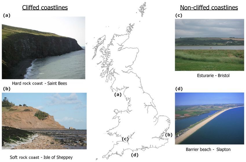
4318 A. Payo et al.: Development of an automatic cliff delineation
lineation of cliffs and other shoreline features remains time- The main advantage of an automatic algorithm for cliff
consuming and somewhat dependant on the analyst’s inter- top and toe delineation is that the uncertainty associated with
pretation. manual digitization, which is subject to human error and
subjective judgement, can be quantified and reduced. How-
ever, given the complexity of the problem, we acknowledge
1.1 The problem of defining the top and bottom of a
that this delineation will inevitably involve some ambiguity,
cliff
which will only be resolved by human screening of the out-
puts. Therefore, a major requirement of any automatic cliff
Defining a cliff is a difficult problem. The top and bottom of toe and top delineation procedure is some means of readily
a cliff are often readily apparent and implicitly defined along screening the outputs.
stretches of the coast with iconic vertical cliffs, e.g. those
composed of chalk or massively bedded and indurate sed- 1.2 Review of automatic delineation procedures
imentary rocks (Fig. 1a). In less favourable circumstances,
however, the relatively slow and sporadic erosion of cliffs Since cliff edges are linear features which are detectable
may leave a compound surface that (in profile and in plan in digital elevation models (DEMs), automated and well-
view) is composed of partly concave and convex shapes. known methods used to extract break lines can potentially
These compound surfaces may be further complicated by the be adapted to extract cliff edges. The automated methods of
occurrence of pre-existing and uplifted marine terraces, inter- break line extraction can be grouped into four major cate-
vening coastal rivers (some of which may be hanging), and gories (Palaseanu-Lovejoy et al., 2016): (1) deriving lines
anthropogenic structures such as transport corridors (usually from intersecting planes (i.e. Briese, 2004; Brzank et al.,
roads). These complications make the top of such a com- 2008; Choung et al., 2013), (2) extracting lines through
pound cliff profile difficult to define. a neighbourhood analysis of DEM elevation values (i.e.
The situation is made more complex still when it is recog- Rutzinger et al., 2012; Hardin et al., 2012; Mitasova et al.,
nized that cliff erosion is, on a human timescale, episodic. 2011), (3) applying edge detection filters and segmentation
Cliff erosion occurs typically by land-sliding. Landslides methods developed for image processing (Sui, 2002; Richter
are well known to be of a variety of types and, in general, et al., 2013; Lee et al., 2009) and (4) automatic elevation pro-
their frequency and magnitude follow a power-law distribu- file elevation extraction analysis (Liu et al., 2009; Palaseanu-
tion (Hurst et al., 2013). This means that larger landslides Lovejoy et al., 2016). The method that we present here be-
occur much less frequently than smaller ones. An obvious longs to the last category and its rationale is described below.
and clearly visible “top” of the cliff may simply be the top Liu et al. (2009) developed a method based on elevation
of more frequent but relatively small landslides. Earlier and profile extraction across the cliffs and the observation that
larger landslides may be visible in a topographic analysis of generally the variation in the slope along the elevation pro-
the sort described here, but they may also be subsumed into file is greater at the top and the toe of the cliff than anywhere
anthropogenic landforms that form the boundaries of trans- else along the profile. However, this may not be the case for
port infrastructure (Fig. 1b). complex cliffs with roads or terraces cut through the cliff gra-
At present, cliffs are eroding in response to a relatively sta- dient, cliffs with different erosional profiles or slope gradi-
ble late Holocene sea-level, established between 7 and 6 kyr ents, or cliffs formed at the base of hills. Palaseanu-Lovejoy
BCE, but the extent to which cliff erosion is accelerating et al. (2016, hereinafter PL2016) proposed an alternative
or has reached a dynamic steady state is also a function of method based also on profile extraction from high-resolution
the tectonic setting (e.g. whether land is actively uplifting or DEMs but that does not involve variation in slopes between
subsiding) and the form of the near shore, which modulates the profile point (i.e. cliff top and toe are delineated as the
wave energy as it propagates to the cliff line. Thus, the cliff maximum and minimum, respectively, of the detrended pro-
top, if considered as the upper moving boundary of a dy- file). The PL2016 automatic delineation method has proven
namic process of cliff failure, is by no means easy to define: useful in resolving a range of types, from almost-vertical
it may not always be the topographic high along the coast- cliffs with sharply defined top and toe inflection points to
normal profile. Still, more complexity arises from the obser- complex cliff profiles. The PL2016 method relies on the user
vation that cliffed coastlines are often interrupted by other being able to generate a reference generalized vector shore-
non-cliffed coastal landforms such as estuaries and beaches line which is free from tight bends and, as much as possible,
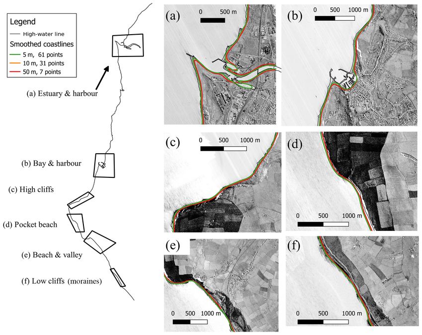
(Fig. 1c, d). For example, based on the European Com- is parallel to the general direction of the cliffs. The gener-
mission (1998 – the CORINE project érosion cotière), the ation of the reference shoreline is, however, not part of the
14 321 km of coastline of the British coast can be classified automatic delineation method itself. Such a generalized vec-
morpho-sedimentologically as cliffs (67 %: 56 % hard rock tor shoreline is not always possible to achieve for very ir-
and 11 % soft rock), sand beaches (11 %), shingle beaches regular coastlines (i.e. sequences of small bays and capes)
(7 %), heterogeneous beaches (4 %) and muddy and estuar- such as parts of the northern and western coastlines of Great
ine coasts (10 %) (May and Hansom, 2003). Britain. Also, the length of the profile is a key parameter in
Geosci. Model Dev., 11, 4317–4337, 2018 www.geosci-model-dev.net/11/4317/2018/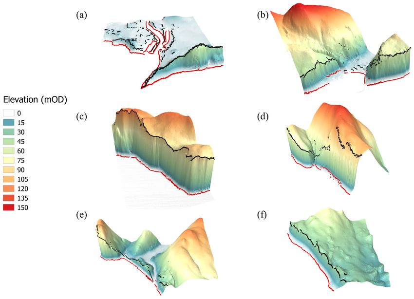
A. Payo et al.: Development of an automatic cliff delineation                                                                               4319

Figure 1. The problem of defining the top and bottom of a cliff is not trivial. For example, most of Britain’s coastline is made of cliffs (hard
and soft) but also beaches and estuarine environments. (a) Cliff top and toe are readily apparent for the hard rock coast of Saint Bees but
not as clear at the soft-cliffed coastline of the Isle of Sheppey where landslides are ubiquitous (b). Cliffed coastlines are often interrupted by
other landforms such as estuaries (c) and beaches (d).

this approach, but as shown by PL2016, the method is robust                ent DEM resolutions and user-defined parameter settings (ex-
enough that the position of the top and toe of the cliff does              plained in detail below). Model outputs are compared with
not change with the length of the profile, as long as the cliff            the uncertainty in manually digitized cliff toe and top as part
is the most prominent geomorphic feature present. Ensuring                 of a sensitivity analysis of our approach.
that the cliff is the most prominent feature can be achieved                  Our software and documentation are available under the
by shortening and/or lengthening the profile length along the              Open Government Licence (see code availability section).
different coastline segments as done by PL2016 during pre-
processing. But even if the pre-processing is done carefully,
it is likely that – due to natural variability in geomorphic fea-          2     Study site and methods
tures – the cliff is not the most prominent feature in some
locations. Thus this need to fine-tune the profile length for              2.1    Digital elevation model source and study sites
different coastal segments during the pre-processing stage
detracts from the benefits of having an automatic delineation              Our automated procedure requires a bare-earth DEM. The
procedure. It remains unclear how the results might differ                 only requirement of the proposed method regarding the DEM
by using a fixed coastline normal versus a fine-tuned normal               is that it should include the cliff toe and top (i.e. cover
length for each coastal segment.                                           from the shoreline to sufficiently far inland to capture the
    Here, we present an automatic cliff toe/top delineation al-            cliff top). The algorithm is agnostic regarding the method
gorithm based on profile elevation extraction from a DEM,                  used to collect the data (i.e. airborne radar, terrestrial or un-
using a fixed profile length, and an automatic generation of a             manned aerial vehicle (UAV), lidar, etc.). We have used sev-
generalized coastline that is suitable for very irregular coast-           eral DEMs from the UK as an example of very irregular plan-
line shapes. The proposed method is demonstrated at several                form coastline but the method is in principle transferable to
study locations along the British coastline using a DEM with               any other DEM. Here, we have used different resolutions
national coverage. We compare the outputs of the proposed                  of the NEXTMap DEM for Britain. NEXTMap for Britain
method with the outputs produced by the PL2016 method.                     is a 5 m resolution DEM derived by airborne radar technol-
We also explore the reproducibility of the results using differ-           ogy by Intermap Technologies. The elevation data were cap-

www.geosci-model-dev.net/11/4317/2018/                                                          Geosci. Model Dev., 11, 4317–4337, 2018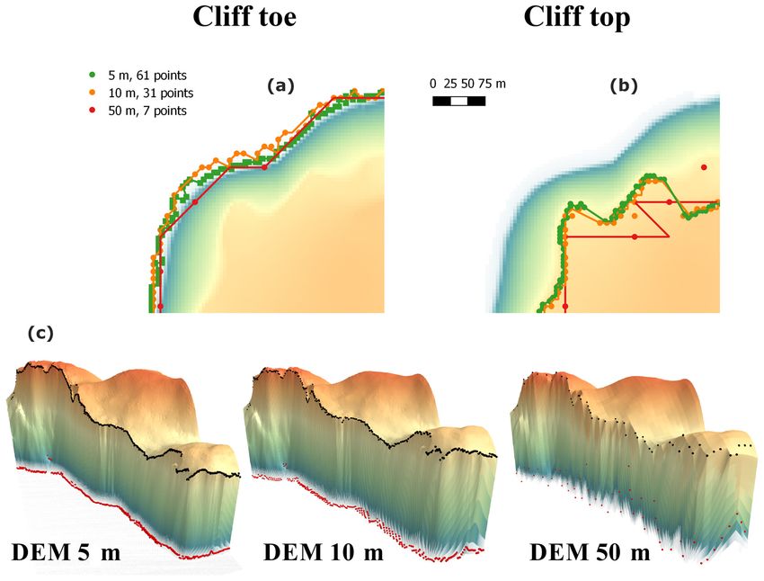
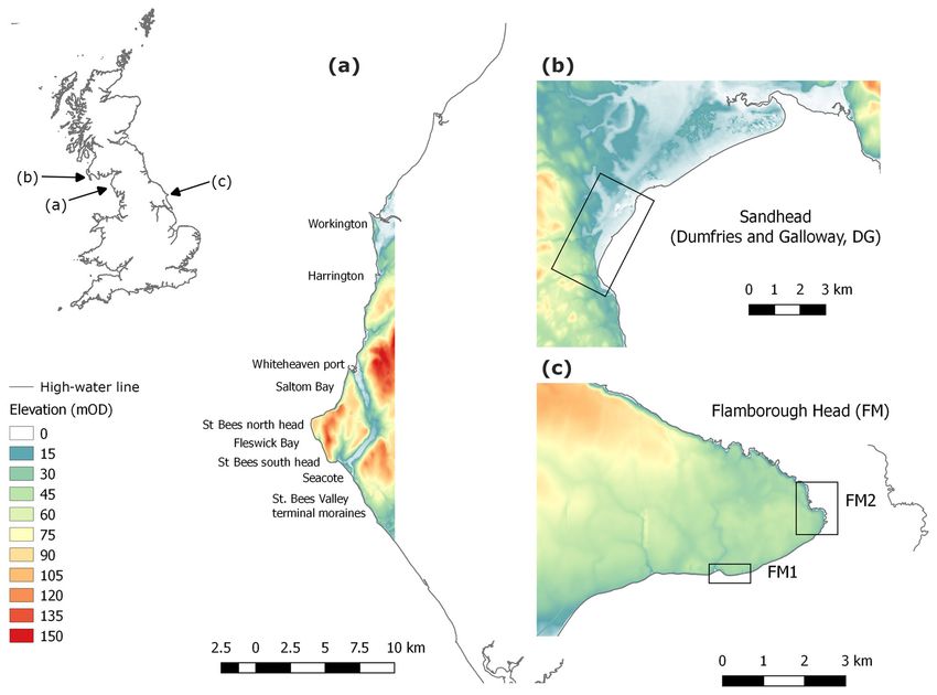
4320                                                                A. Payo et al.: Development of an automatic cliff delineation

Figure 2. The NEXTMap DEM (mOD: metres ordinance datum) of selected study sites around Britain’s coastline; (a) St Bees head in
northwest England, used for the model sensitivity analysis. The name of the main locations cited in the text are shown along this coastal
stretch, (b) Sand Head and (c) Flamborough head sites are non-active and active cliffed coastlines sites used for the manually digitized
uncertainty analysis. At Flamborough, two study sites were selected with cliffs of similar heights but with relative uniform coastline (FH1)
and very irregular coastline shapes (FH2).

tured during 2002–2003 and provide elevation point data on              algorithm behaviour. For the sensitivity analysis and model-
a 5 m grid, which has subsequently been interpolated using              to-model comparison, we have focused on a coastal cliff-
a bespoke algorithm to derive the underlying “bare earth”               dominated region with irregular plan shape to make our find-
terrain model i.e. removing surface features such as build-             ings more transferable to other similar cliffed coastlines else-
ings and trees. NEXTMap height data have a vertical ac-                 where. For the manually digitized cliffs analysis, we have se-
curacy of around 1 m ± RMSE and a horizontal accuracy of                lected a challenging coastal region (i.e. very irregular shape,
2.5 m ± RMSE on slopes less than 20◦ . NEXTMap uses the                 complex cliff profile sections intercalated with non-cliffed
OSGB36 horizontal datum and all elevations are relative to              sections) to highlight the importance of screening the results
the ordnance datum Newlyn vertical datum. Radar cannot                  and running the algorithm iteratively until the manually digi-
penetrate water and therefore the DEM records the elevation             tized and automatically delineated cliff top and toe locations
of the water surface at the time of image acquisition. Higher           converge.
resolution DEMs of 10 and 50 m were obtained by averaging                  For our sensitivity analysis, we selected a 30 km coastal
the elevation of the 5 m DEM.                                           stretch centred at St Bees Head in northwest England. This
   The aims of the sensitivity, model-to-model comparison               study area, which is part of the coast of the county of Cum-
and manually digitized cliff analyses are different and there-          bria, contains an assortment of different coastal morpholo-
fore the places selected to conduct each analysis are different         gies but it is mostly dominated by high cliffs (Fig. 2a). The
too. Our sensitivity analysis and model-to-model compari-               southern section of the study area, south of St Bees Head, is
son investigates the way in which the variation in the output           fully exposed to the sea conditions from the Irish Sea, while
can be attributed to variations in the different input factors          the northern section is dissected by more sheltered estuarine
(Pianosi et al., 2016) or different automatic delineation pro-          environments. The rock has been eroded by wave action to
cedures, respectively. The manually digitized cliffs analysis           produce the spectacular 80 m high vertical cliffs stretching
illustrates the importance of the data output screening and             from the Seacote foreshore to Saltom Bay. At Fleswick Bay,

Geosci. Model Dev., 11, 4317–4337, 2018                                                    www.geosci-model-dev.net/11/4317/2018/
A. Payo et al.: Development of an automatic cliff delineation                                                                                          4321

Table 1. Summary of output files produced by the proposed method: name, description and type.

  Output name                                         Description                                                                           Type
  XX.out                                              Log of user set-up and run performance                                                ASCII
  XX.log                                              Log of simulation run details                                                         ASCII
  sediment_top_elevation.tif                          DEM read by the script and used to delineate the cliff metrics.                       GeoTIFF
  rcoast.tif                                          Raster coastline. Raster cells that are marked as on the coastline have a value of    GeoTIFF
                                                      1 value or 0 otherwise
  coast_point_XX.shp                                  Point vector with all the raster coastal points and four attributes; nCoast is        point shape file
                                                      the coast number, nProf is the profile number which is unique for each coast-
                                                      line segment, CoastEl is the elevation in metres of the coast point (i.e. not all
                                                      coast points have the same elevation but this varies according with the DEM),
                                                      chainage or distance in metres in the horizontal plane from the sea point (i.e. it
                                                      should be 0 m for all coast points by definition).
  coast_XX.shp                                        Point vector with the smoothed coastline. The number of points of                     point shape file
                                                      coast_XX.shp is equal to the number of points on coast_point_XX.shp
  rcoast_normal.tif                                   Raster coastline normal. Raster cells that are marked as on the coastline normal      GeoTIFF
                                                      have a value of 1 or 0 otherwise.
  normals_XX.shp                                      Line vector with the valid coastline normals                                          line shape file
  invalid_normals_XX.shp                              Line vector with the non-valid coastline normals                                      line shape file
  coast_nCoast_profile_nProf_XX.csv                   CSV file with the elevation profile for profile number “nProf” on coast number        ASCII
                                                      “nCoast” and DEM named XX. Each file contains the chainage (i.e. horizontal
                                                      distance from seaward limit), absolute (x, y) location, elevation above vertical
                                                      datum and detrended elevation.
  cliff_toe_XX.shp                                    Point vector with cliff toe position and four attributes; nCoast is the coast num-    point shape file
                                                      ber, nProf is the profile number which is unique for each coastline segment,
                                                      bisOK is a Boolean flag that will be 1 if the profile is valid or 0 otherwise,
                                                      CliffToeEl is the elevation in metres of the cliff toe, and chainage of the toe
                                                      point.
  cliff_top_XX.shp                                    Point vector with cliff-top position and four attributes; nCoast is the coast num-    point shape file
                                                      ber, nProf is the profile number which is unique for each coastline segment,
                                                      bisOK is a Boolean flag that will be 1 if the profile is valid or 0 otherwise,
                                                      CliffTopEl is the elevation of the cliff top, and chainage of the top point.

XX is the user-defined main output and log files name. All elevations are in metres.

Table 2. Summary of the local sensitivity analysis of cliff toe and top locations to different model set-up.

                                                                                                    DEM resolution
                                                                        5m                     10 m                       50 m
                                                           61 pt        Reference                           to DEM resolution only
                       Window size smoothing
                                                           31 pt        to smoothing only
                                                           7 pt                                to DEM resolution, smoothing and threshold
                                                           0.5 m        Reference                                  all combined
                       Vertical threshold                  0.01 m       to threshold only
                                                           1.5 m

                     Average, standard deviation, maximum, minimum shortest distance between reference and this output.

a shingle beach lies on large sandstone platforms. At the west                              by trapped beach material. The coastline for about 100 m im-
end of the St Bees Valley, terminal moraines dating from the                                mediately to the north of Whitehaven Harbour is protected by
last glacial period (∼ 12–14 000 BP) are exposed at the coast                               an armoured stone bank. A railway embankment fronts the
as bluffs. The west pier at Whitehaven Harbour forms a sig-                                 natural cliffs along the coastline between Whitehaven and
nificant barrier to the movement of beach material further                                  Harrington. At the northern limit of the study region is the
north. A small beach exists to the south of west pier, formed                               port city of Workington. Around Workington slag banks from

www.geosci-model-dev.net/11/4317/2018/                                                                            Geosci. Model Dev., 11, 4317–4337, 2018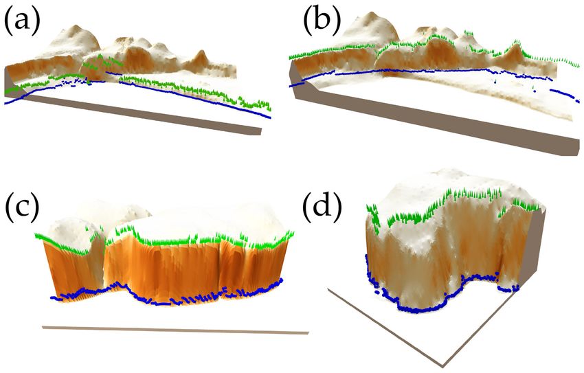
4322                                                               A. Payo et al.: Development of an automatic cliff delineation

                                                                      11.5 ka BP). The second cliffed section (FM2) was located
                                                                      on the north face of Flamborough Head on the chalk cliffs,
                                                                      which are overlain by the glacial till deposits. On both sec-
                                                                      tions, FH1 and FH2, cliff heights are of the order of 20 m but
                                                                      the coastline has a more irregular shape on FH2 than FH1.
                                                                      Section 3 (DG) is located near Sandhead, Dumfries and Gal-
                                                                      loway (UK) and is an inactive cliffed coastline. At section
                                                                      DG, maximum profile elevations are of the order of 20 m.

                                                                      2.2   Automatic delineation of cliff metrics

                                                                      The automatic delineation procedure quantifies cliff top and
                                                                      cliff toe position, and cliff height, following the steps shown
                                                                      as a flow chart in Fig. 3, illustrated further in Fig. 4 and de-
                                                                      scribed in detail below. All the resulting geospatial outputs
                                                                      produced by the proposed method are listed in Table 1.

                                                                        – Extracting the coastline from a DEM.
                                                                            Figure 4a shows the input DEM that we use to illus-
                                                                            trate the methodology. The first step is to delineate the
                                                                            shoreline at a user-defined elevation. Coastline cells are
                                                                            delineated using a wall-follower algorithm (Sedgewick,
                                                                            2002). The wall is at the interface between cells above
                                                                            and below the user-defined elevation. Raster cells “on”
                                                                            the shoreline are marked (Fig. 4b); the coastline is also
                                                                            stored as a vector object. Depending on the coastal ge-
                                                                            omorphology and extent of each DEM tile, more than
                                                                            one coastline segment may be traced on the DEM. Each
                                                                            coastline segment is given an ID number (Ncoast ). The
                                                                            wall-follower algorithm used to delineate the coastline
                                                                            searches the tile edges to find the start of any coast-
                                                                            line. The coastline of islands (i.e. land topography that
                                                                            does not cross the edges of the DEM) is not delineated
                                                                            (Figure 5). To resolve the islands, the tile needs to be
                                                                            zoomed-in to ensure that the edges of the land topogra-
                                                                            phy intersect any of the tile edges.

                                                                        – Generate a generalized (smoothed) coastline.
                                                                            The resulting coastline is then smoothed to eliminate
                                                                            artefacts resulting from the resolution of the DEM, due
Figure 3. Flow chart of the proposed automatic delineation algo-            to local geomorphic variability associated with the het-
rithm.                                                                      erogeneity of natural landscapes, and the presence of
                                                                            artificial features at the coast, in order to produce a
                                                                            generalized coastline. This is done either by running
blast furnace plants cover large sections of the coast, which               a moving-average window across the positional x–y
also contains alluvial deposits from the River Derwent.                     coordinates or by Savitzky and Golay (1964) smooth-
   For the manually digitized cliffs analysis, we selected                  ing, which involves fitting successive subsets of ad-
three 1 km sections that represent active cliffed coastlines                jacent data points with a low order polynomial using
of different height and plan shape (Flamborough Head,                       least squares regression. The user needs to decide which
north and south sections; and one section that represents a                 method better fit their perception of a generalized coast-
non-active, i.e. Holocene, cliff: Sandhead; Fig. 2b, c). The                line. The resulting smoothed coastline comprises a com-
first cliffed section (FH1) was located on the south side of                pound vector object. This is made up of two sets of
Flamborough Head, Yorkshire (UK), within highly erodible                    consecutive points: a set holding the location of each
glacial tills deposited during Devensian glaciations (ca. 35 to             smoothed coastline point and a set holding the orig-

Geosci. Model Dev., 11, 4317–4337, 2018                                                 www.geosci-model-dev.net/11/4317/2018/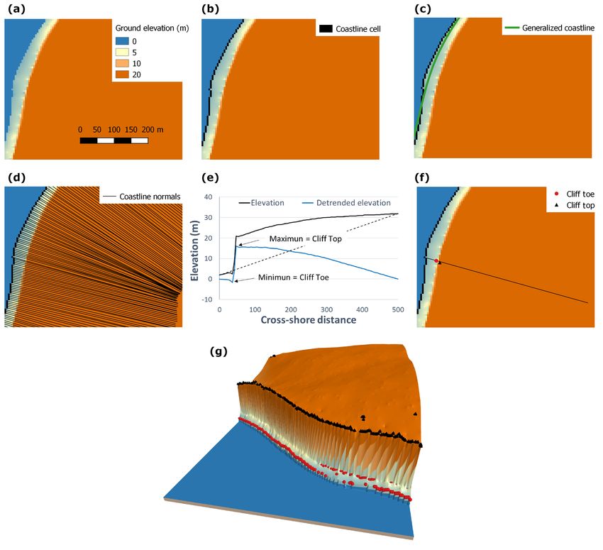
A. Payo et al.: Development of an automatic cliff delineation                                                                             4323

Figure 4. Step by step Illustration of the proposed method to generate the generalized coastline and extract the cliff toe and top elevations
and locations; (a) the input digital terrain model (DTM) and (b) the cells on the coastline are marked and (c) smoothed to create a generalized
coastline vector; (d) coastline normals are delineated starting at the cells marked as on the coastline and perpendicular to the straight line
connecting the before and after smoothed-coastline point; (e) profile elevation is extracted along each normal and cliff top and toe are located
as the maximum and minimum elevation of the detrended elevation profile; (f) shows the location of the cliff top and toe along the elevation
profile shown in panel (e); (g) shows the DTM in 3-D and the output locations of cliff toe (red circles) and top (black circles).

     inal non-smoothed cell location of the coastline point                     section). Coastline normal transects that are too short
     (Fig. 4c).                                                                 (i.e. extend for only two raster cells) are considered in-
                                                                                valid for the delineation of the cliff metrics: these are
  – Extract transects normal to the coast.                                      flagged as “non-valid”. Intersecting coastline normals
     We then generate cross-shore transects, from which we                      are flagged as “intersecting but not truncated”.
     extract the coastal topography. These cross-shore tran-
     sects are located perpendicular to the smoothed coast-                  – Morphometric identification of the cliff top and toe.
     line, extending inland from each coastline cell for a                      Coastline-normal elevation profiles are then sampled
     user-defined distance (Fig. 4d). Normals that intersect                    from the DEM cells under each valid coastal normal.
     the coastline more than once (e.g. barrier beaches, head-                  The elevation of each point of the coastline normal is
     lands) are flagged as “hitting the coast” profiles; their                  determined using the elevation of the centroid of the
     length is reduced (i.e. the profile is shortened to the seg-               closest raster cell (thus coarser resolution DEMs will
     ment between the first and the second shoreline inter-                     produce more jagged elevation profiles). A topographic

www.geosci-model-dev.net/11/4317/2018/                                                         Geosci. Model Dev., 11, 4317–4337, 2018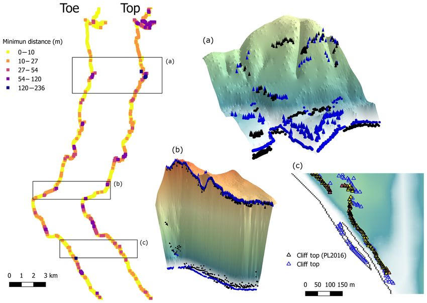
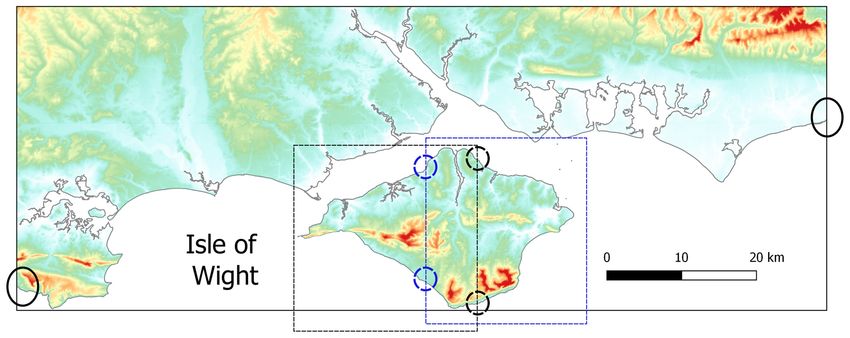
4324                                                                  A. Payo et al.: Development of an automatic cliff delineation

Figure 5. The algorithm used to delineate the coastline searches the edges of the tiles to find the start point of the coastline. The solid grey
line represent the coastline over the coloured DEM (i.e. the warmer the colour the higher the elevation). The coastline cuts the edges of the
DEM at the locations indicated by the solid black circles. The coastline of the Isle of Wight does not cut the edges of the DEM and therefore
the user needs to define two smaller DEM domains (represented as dashed black and blue rectangles for the west and east side of the isle).
The isle coastline now cuts the smaller domains at the locations indicated by the blue and black dashed circles. It is recommended to allow
some overlap between the smaller domains to ensure that the cliff metrics are well resolved near the edges.

Figure 6. Location of six different coastal morphologies around St Bees Heritage Coast and smoothed coastline obtained for different DEM
resolutions and window sizes used for smoothing. Original radar images used to build the NEXTMap DEM shown in grey scale. Smoothed
line for the 10 m DEM with 31 points window size (orange line) is almost identical to the line obtained for the 5 m DEM with 61 points
window size (green line) and not always visible.

Geosci. Model Dev., 11, 4317–4337, 2018                                                       www.geosci-model-dev.net/11/4317/2018/
A. Payo et al.: Development of an automatic cliff delineation                                                                       4325

Figure 7. Generalized coastline and coastline normals used for the proposed method and the PL2016 method. (a) Smoothed coastline (solid
black) on top of high-water line (solid grey). Close ups around Whitehaven and Workington harbours illustrate the differences between both
lines. (b) Coastline normals derived using the proposed methodology. (c) Coastline normals derived using PL2016. The different colours
represent the different segments used.

      trend line is then calculated as the elevation difference        erence, we used the cliff metrics outputs for the DEM of 5 m
      between the start and end points on the profile, divided         resolution, a 61-cell moving-average window for coastline
      by the horizontal profile length (Fig. 4e). The detrended        smoothing, and 0.5 m as the vertical threshold. This distance
      profile elevation is then calculated as the residual when        seems to be large enough to produce a smooth coastline and
      the topography is compared with the trend line. Finally,         small enough to resolve the numerous headlands and bays
      the cliff top and cliff toe are identified as the maximum        along this part of the British coastline. To explore the local
      and minimum detrended elevations (Fig. 4f). All cliff            sensitivity to coastline smoothing, we have also used 31-cell
      toe and top points for the input DEM, as identified using        and 7-cell moving-average window sizes that are equivalent
      this procedure, are shown as a 3-D model in Fig. 4. Note         to ∼ 165–220 and ∼ 35–50 m windows, respectively. We se-
      that an optional user-defined elevation threshold may be         lected the vertical threshold of 0.5 m as the reference thresh-
      used to avoid false peaks. If the absolute value of the          old because it is of the same order of magnitude as the verti-
      peak elevation (depression) is lower than the threshold          cal accuracy of the radar elevation data used by NEXTMap.
      elevation, it is assumed that the points at the end (start)      The reference threshold elevation is relative to the detrended
      of the profile are the cliff top (toe). This “elevation san-     elevation and it can be smaller than the DEM resolution. To
      ity check” is required to avoid small bumps on rather            explore the local sensitivity to vertical threshold value, we
      slope-uniform profiles (i.e. non-cliffed coastlines) being       also used vertical thresholds of 0.01 and 1.5 m.
      picked up as cliff tops or toes.                                    Figure 6 shows the smoothed coastline obtained, using
                                                                       these different DEM resolutions and different smoothing
2.3   Sensitivity analysis and model vs. model                         window sizes, for six different coastal morphological en-
      comparison                                                       vironments: (a) estuarine, (b) bay with harbour, (c) un-
                                                                       interrupted high-cliffed coastline, (d) pocket beach sur-
We assessed output sensitivity to (1) the DEM resolution, us-          rounded by high cliffs, (e) beach at the seafront of a relic
ing DEMs of 5, 10 and 50 m of the same study region; (2) the           valley, and (f) low-cliff coastline (i.e. eroding moraines).
degree of smoothing of the generalized coastline; and (3) the             When the number of points for the window size is chosen
threshold used to avoid false cliff top/toe locations. Table 2         to make the window length similar under different DEM res-
summarizes results from these sensitivity analyses. As a ref-

www.geosci-model-dev.net/11/4317/2018/                                                     Geosci. Model Dev., 11, 4317–4337, 2018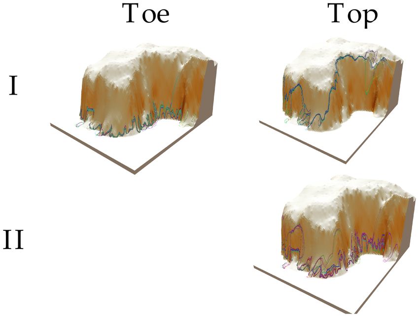
4326                                                                   A. Payo et al.: Development of an automatic cliff delineation

Table 3. Differences and commonalities of proposed method versus PL2016 method.

                      Proposed method                                            PL2016
   Differences        – it is compiled so it is quicker (C++)                    – the code is readable so profile extraction function
                      – less pre-processing                                      from the DEM along transects is slower (R)
                      – computes only cliff top and toe                          – pre-processing work to set up the buffers for generat-
                      – process concave short profiles (i.e. incomplete cliff    ing transects is necessary
                      profiles look like a check mark)                           – computes secondary inflections on the face of the cliff
                      – can deal with very long and narrow promontory by         and if desired identifies the top and 2 toes of a sand bar
                      adjusting the normal length automatically                  in front of the cliff (one toe on each side of the sand bar
                      – transects start at a user-defined level and projected    top)
                      inland perpendicularly to an automatically delineated      – reject completely concave profiles (profiles that look
                      smoothed coastline                                         like a check mark)
                                                                                 – cannot deal with long and narrow promontory, unless
                                                                                 more involved pre-processing is done. par – transects
                                                                                 are projected seaward and inland perpendicularly to a
                                                                                 externally delineated coastline
   Commonalities      – after the profile is extracted the 2 codes to extract top and toe are similar using the same logic
                      – both methods output the profile elevation for further processing
                      – rejects short profiles with Nmin or less elevation points on land, where Nmin = 3 and 5 for proposed method
                      and PL2016 (there is nothing preventing the methods to be set up for the same Nmin )

olutions, the resulting smoothed coastlines are very similar.             the line segment that joins the point to the line and is per-
In particular, the smoothed coastlines for the 5 m DEM and                pendicular to the line. We calculated the average, standard
61 points and the 10 m DEM and 31 points are almost identi-               deviation, maximum and minimum shortest distances for all
cal. In all cases, the smoothed coastline differs from the high-          source points.
water line, which is expected when using a still-water level of              For the model-to-model comparison, we compared the
1.0 m above the ordinance datum (OD) to delineate the coast-              model outputs for the reference set-up with the PL2016
line. By choosing a water level of 1.0 m above OD, we have                model outputs. Both methods differ regarding the pre-
avoided delineating artificial coastal infrastructure, such as            processing that is required (Table 3). The PL2016 method re-
the Whitehaven Harbour, where elevation has not been fully                quires more pre-processing than our approach since PL2016
removed from the DEM. Around the Workington harbour,                      needs to create a generalized coastline, split the coast into
the estuary cuts the edges of the DEM and the model auto-                 segments and then associate a buffer width with each seg-
matically creates two coastlines (a short one to the north side           ment. For the St Bees study region of circa 30 km, the coast-
of the Workington harbour, and a longer one to the south).                line was divided into 25 segments; buffer width ranged from
   Choosing metrics to compare model outputs is not                       20 to 400 m (Fig. 7). Our method delineates the smoothed
straightforward. The number of cliff-top/toe points varies                coastline automatically and does not require the coastline
with the DEM resolution (because the method delineates one                to be divided into segments. However, coastline segments
coastline normal through every coastal cell point) making a               will be created if the delineated coastline cuts the edges of
profile-to-profile comparison infeasible (because profile el-             the DEM domain. We used the smoothed coastline produced
evation and orientation will also vary with DEM resolution                by our algorithm, using the reference set-up, as the general-
and selected coastline smoothing). Thus, we chose a point-to-             ized line required for the PL2016 method. Both methods are
line-distance approach. Points are the cliff-top/toe location             therefore quite similar with regard to coastline selection. The
outputs; as a reference line, we converted the cliff-toe/top              main difference concerns the way that the coastline normals
points into a cliff-top/toe line for the reference model set-             are defined. After some trial and error, we chose a profile
up. The minimum distance between the cliff toe/top loca-                  length of 500 m as our user-defined fixed length. As a metric
tions and the reference line was calculated using the Quan-               of the differences in outputs, we again use the QGIS “Dis-
tum geographic information system (QGIS) 2.18.3 “Distance                 tance to nearest hub” to calculate the differences in the cliff
to nearest hub” tool. Given a layer with source points (i.e.              top and toe locations outputs produced by the method pro-
cliff toe/top points) and another layer representing destina-             posed here and in PL2016.
tion points or lines (i.e. reference cliff toe/top line), this “Dis-
tance to nearest hub” tool computes the distance between
each source point and the closest destination one. The short-
est distance between any point and a line is the length of

Geosci. Model Dev., 11, 4317–4337, 2018                                                     www.geosci-model-dev.net/11/4317/2018/
A. Payo et al.: Development of an automatic cliff delineation 4327
Figure 8. Cliff toe and top outputs for a high-cliffed coastline section and different DEM resolutions and smoothing window size. Upper
panels show the locations of the cliff toe (a) and cliff top (b). Bottom panels show 3-D models with the cliff toe and top as red and black
spheres, respectively. Vertical dimension of 3-D models have been exaggerated 10 times.
2.4 Manually digitized profile analysis and iterative mum shortest distances for all source points. This provides us
output screening method with both a quantitative assessment of the uncertainty in hu-
man interpretation of cliff top and toe lines from aerial pho-
As outlined in the Introduction section, a major requirement tography as well as a number of target cliff and top and toe
of any automatic cliff toe/top delineation procedure is some lines to test the proposed algorithm behaviour.
means of readily screening the outputs. In this section, we Building on (1) the uncertainty in the human interpretation
describe how we have developed a methodology to itera- of cliff top and toe lines from aerial photography, (2) sensi-
tively screen over the model results and run the automatic tivity analysis results and (3) model outputs (see Table 1) we
delineation algorithm to achieve a desired model behaviour developed an iterative output screening method to achieve the
or identify any bias on the target lines. desired model behaviour and identify bias on the target lines.
The target cliff top and cliff toe locations are obtained from We clustered the manually digitized lines to broadly capture
a cluster of 24 manually digitized lines from aerial photogra- the different interpretation of coastal cliff toe and top. The
phy. A group of 24 participants with a range of geological ex- different clusters were then linked to the different model set-
pertise participated in the experiment, each interpreting data up parameters. We then illustrate a model output screening
for three 1 km sections (FH1, FH2 and DG; see Fig. 2b, c). method and iterative parameter selection for users to achieve
Using a geographic information system (GIS; Google Earth desired model behaviour.
Pro 7.1.8.3036, 32-bit), participants attempted to delineate
cliff top and toe lines without any prior knowledge of their
location. As with the sensitivity analysis, we used a point- 3 Results
to-line metric to calculate the main statistics of the manu-
ally digitized results. As a reference line, we generated a 3.1 Output sensitivity to DEM resolution, coastline
mean cliff top and toe line for each of the study sections smoothing and vertical threshold
from the participant data. We extracted the cliff top and toe
points from each one of the manually digitized lines and cal- Figure 8 shows the cliff toe and top locations for a high-
culated the average, standard deviation, maximum and mini- cliffed coastal segment at the St Bees study site for different
www.geosci-model-dev.net/11/4317/2018/ Geosci. Model Dev., 11, 4317–4337, 20184328 A. Payo et al.: Development of an automatic cliff delineation
Table 4. Cliff toe average, standard deviation, maximum difference and number of samples for the sensitivity analysis to DEM resolution,
window size for coastline smoothing and vertical threshold.
Cliff TOE
Average differences
Window size DTM resolution Vertical threshold DTM resolution
5m 10 m 50 m 5m 10 m 50 m
61 pt 0 4 25 0.5 m 0 4 25
31 pt 1 3 26 0.01 m 1 4 25
7 pt 2 4 25 1.5 m 1 5 26
Standard deviation
Window size DTM resolution Vertical threshold DTM resolution
5m 10 m 50 m 5m 10 m 50 m
61 pt 0 9 38 0.5 m 0 9 41
31 pt 6 4 41 0.01 m 4 7 41
7 pt 13 9 38 1.5 m 9 12 43
Maximum differences
Window size DTM resolution Vertical threshold DTM resolution
5m 10 m 50 m 5m 10 m 50 m
61 pt 0 299 351 0.5 m 0 299 351
31 pt 229 68 282 0.01 m 159 221 351
7 pt 217 204 282 1.5 m 289 299 368
Number of samples
Window size DTM resolution Vertical threshold DTM resolution
5m 10 m 50 m 5m 10 m 50 m
61 pt 3213 591 0.5 m 3213 591
31 pt 6605 3274 596 0.01 m 6598 3213 591
7 pt 6587 3279 611 1.5 m 6598 3213 591
DEM resolutions and for different smoothing window sizes. the smoothing window and the vertical threshold (i.e. differ-
The cliff metrics for the 5 m DEM 61-point window size and ences always smaller than 2 m). Standard deviation is largest
10 m DEM 31-point window size are very similar and are (about 40 m) for the DEM of 50 m resolution, and is about
clearly different to the metrics obtained for the 50 m DEM 10 m for the outputs from the DEM of 5 and 10 m resolutions.
7-point window size. The cliff metrics for the 3-D models The maximum difference is 368 m for the DEM of 50 m and
illustrate how the cliff top and toe locations relate to the res- vertical threshold of 1.5 m.
olution of the DEMs. Figure 9 shows the cliff metrics for all Table 5 shows the results for the cliff-top sensitivity anal-
six regions and the 3-D model derived from the 5 m DEM. ysis. Average differences between the cliff-top location out-
While our approach is designed to resolve cliffed coastlines, puts and the reference outcome vary between 0 and 37 m,
it also seems to be able to resolve very irregular coastline again being most sensitive to changes in DEM resolution (i.e.
shapes such as a pocket beach between high cliffs (Fig. 9d), average differences of 6 and 32 m for the 10 and 50 m DEM
a bay (Fig. 9b), and estuarine environments (Fig. 9a). resolutions, respectively). Cliff-top location is (again) less
Table 4 shows the results for the cliff-toe sensitivity anal- sensitive to changes in the size of the smoothing window and
ysis for the St Bees study case. The average difference be- the vertical threshold (i.e. differences always smaller than
tween the cliff-toe location outputs and the reference out- 8 m). Standard deviation is largest (about 60 m) for the DEM
come varies between 1 and 26 m. It is most sensitive to of 50 m resolution, and is about 10–20 m for the outputs from
changes in DEM resolution (i.e. average differences of 4 and the DEM of 5 and 10 m resolutions. The maximum difference
25 m for the 10 and 50 m DEM resolutions, respectively). is 502 m for the DEM of 50 m and 7-point smoothing window
Cliff-toe location is less sensitive to changes in the size of
Geosci. Model Dev., 11, 4317–4337, 2018 www.geosci-model-dev.net/11/4317/2018/A. Payo et al.: Development of an automatic cliff delineation 4329
Table 5. Cliff top average, standard deviation, maximum difference and number of samples for the sensitivity analysis to DEM resolution,
window size for coastline smoothing and vertical threshold.
Cliff TOP
Average differences
Window size DTM resolution Vertical threshold DTM resolution
5m 10 m 50 m 5m 10 m 50 m
61 pt 0 6 32 0.5 m 0 6 33
31 pt 3 5 32 0.01 m 0 6 31
7 pt 5 8 29 1.5 m 8 6 37
Standard deviation
Window size DTM resolution Vertical threshold DTM resolution
5m 10 m 50 m 5m 10 m 50 m
61 pt 0 11 62 0.5 m 0 11 33
31 pt 10 21 63 0.01 m 2 11 31
7 pt 19 33 59 1.5 m 8 14 37
Maximum differences
Window size DTM resolution Vertical threshold DTM resolution
5m 10 m 50 m 5m 10 m 50 m
61 pt 0 186 470 0.5 m 0 186 470
31 pt 153 477 479 0.01 m 54 186 458
7 pt 465 497 502 1.5 m 202 186 470
Number of samples
Window size DTM resolution Vertical threshold DTM resolution
5m 10 m 50 m 5m 10 m 50 m
61 pt 3213 591 0.5 m 3213 591
31 pt 6605 3274 596 0.01 m 6598 3213 591
7 pt 6587 3279 611 1.5 m 6598 3213 591
size. There are about 6500, 3200 and 600 coastal points for 3.2 Model-to-model comparison
the DEMs of 5, 10 and 50 m resolutions, respectively.
Since model outputs are most sensitive to DEM resolu- Our results show that the two automatically delineated cliff
tion, we extended the sensitivity analysis to DEM resolu- top and toe locations are, generally, in good agreement (i.e.
tions of 15, 20, and 35 m. To keep the window size to a distances are less than one cell diagonal). Toe locations are
similar magnitude, we chose the window size for smooth- anticipated to be different since the proposed method uses
ing the coastline to be 21, 15 and 9 points for the 15, 20 a user-defined elevation (e.g. 1.0 m: chosen to avoid delin-
and 35 m resolution DEMs, respectively. We kept the verti- eating the artificial infrastructure near the coast, which had
cal threshold unchanged (0.5 m). Figure 10 shows average not been removed from the DEM) to begin its coastline pro-
differences decreasing as the DEM resolution decreases. To files, while the PL2016 method begins its transects from the
estimate the trend in average differences, we fitted and ex- lowest elevation (i.e. 0 m for the DEM used here). Distances
trapolated a polynomial line of order 3 to the cliff top and toe between cliff metrics of less than one cell diagonal length
calculated differences. This fitted trend line suggests that the (i.e. 7.07 m for a 5 m cell size) are considered within the
minimum differences (i.e. for the smallest DEM resolution) DEM resolution limit and thus, for model-to-model compari-
are 1 and 5 m for the cliff toe and top, respectively. son purposes, identical outputs. The PL2016 method applied
to the St Bees study site produced a set of 6655 toe points
and 6324 top points (i.e. top points are less than toe points
because concave profiles are not used to delineate the cliff
top but the profile is still been used to delineate cliff toe). Our
www.geosci-model-dev.net/11/4317/2018/ Geosci. Model Dev., 11, 4317–4337, 20184330 A. Payo et al.: Development of an automatic cliff delineation Figure 9. 3-D models of different coastal morphology environments with the cliff toe (black spheres) and cliff top (red spheres) delineated using the 5 m DEM and 61-point smoothing: (a) estuarine, (b) bay with harbour, (c) high-cliffed coastline, (d) pocket beach, (e) beach at the seafront of a relic valley and (f) low-cliffed coastline (eroding moraines). Figure 10. The cliff metric outputs (top and toe locations) average difference decreases as the DEM resolution decreases. approach produced a data set of 6598 top and toe points, of between the cliff top and toe locations is shown in Fig. 11. which 68 were flagged as poor-quality points. The minimum The cliff toe locations are in good agreement (i.e. minimum distance between the line formed by the proposed method’s distance less than one cell diagonal) for 78 % of the data, and cliff top and toe outputs and the PL2016 outputs was cal- the cliff top locations are in good agreement for 68 % of the culated: the frequency distribution of the minimum distance locations. The median distance for both top and toe locations Geosci. Model Dev., 11, 4317–4337, 2018 www.geosci-model-dev.net/11/4317/2018/
A. Payo et al.: Development of an automatic cliff delineation                                                                          4331

Figure 11. The proposed method and the PL2016 method outputs are in good agreement. Panels shows the distribution of the minimum
distances between cliff toe and top output locations (for a 5 m grid cell, the cell diagonal is 7.07 m or the length of the hypotenuse of the
square triangle made by two connected sides of the grid cell).

Figure 12. Minimum distance between the cliff toe and top outputs using the PL2016 vs. the proposed method. The coloured squares on the
left of the figure represent the location of the outputs produced by PL2016 and the coloured scale represents the minimum distance to the
outputs produced by this method. Cliff toe/top produced by the proposed method are represented in blue, as spheres/cones for the 3-D plots.
Panels (a) and (b) and show both model outputs at locations where distances were the greatest. The largest differences between methods
correspond with (a) where there is a sharp bend on the coast morphology and the cliff is not the dominant feature, (b) at the toe of a very
steep cliff with a small talus and (c) there is a sandbar welded to the shoreline in front of the cliff.

www.geosci-model-dev.net/11/4317/2018/                                                       Geosci. Model Dev., 11, 4317–4337, 2018
4332                                                                  A. Payo et al.: Development of an automatic cliff delineation

Figure 13. Distance from participant cliff lines to the mean reference lines for each section.

Figure 14. manually digitized cliff top and toe lines (coloured lines) over the DEM for the FH2 site. DEM colours represent slope (darker
colours represent higher slopes). The vertical dimension has been exaggerated 10 times. The roman numbers represent the main clusters of
manually digitized lines.

are always inferior to a cell diagonal. To understand where               The maximum differences in toe (236 m) and top loca-
the outputs from the two methods differ between each other,               tion (206 m) are either in segments, where the coastline
it is necessary to look at the spatial distribution of the differ-        makes sharp bends and the cliff is not the dominant feature
ences.                                                                    (Fig. 12a), or where the cliff has a steep face with a talus at
    Figure 12 shows the spatial differences between the cliff             the toe (Fig. 12b). Both methods were able to delineate the
metric results using the PL2016 algorithm and our approach.               cliff metrics along the eroding moraines, but our approach

Geosci. Model Dev., 11, 4317–4337, 2018                                                          www.geosci-model-dev.net/11/4317/2018/
A. Payo et al.: Development of an automatic cliff delineation 4333
rived histograms for each cliff-top site. The spread of delin-
eations around these peaks is similar to those for the cliff
toes. The smaller range in cliff-toe-line variance suggests that
there is greater certainty in participants defining those lines
from aerial photography. The negative skew within the vio-
lin plot analysis is likely due to tide lines, beach and plat-
form being readily identifiable in the images and therefore
less prone to be misinterpreted as cliff-line features. The bi-
modal nature of the cliff top delineation can be attributed to
participants’ personal definition of what constitutes a cliff
top. This dilemma is highlighted in the FH1 and DG sites.
In the former there are two distinct breaks in slope and par-
ticipants tended to follow either a higher or lower cliff top
line (Fig. 14). This dilemma is not present on the FH2 site
were only one distinct break in slope exists (Fig. 15). Within
the DG site there is a very low cliff (< 1 m) at the top of
the beach and a much more pronounced Holocene cliff line
set back around 100 m from the coastline (Fig. 16). Partic-
ipants tended to prefer either one cliff line or the other. In-
terestingly for the DG site, even if participants selected the
Holocene cliff-top, they were unlikely to use the Holocene
toe line. This is highlighted by the lack of bimodal response
in the DG toe-line histogram.
Figure 17 shows the automatically delineated cliff top and
toe for the DG and FH sites using different input model set-
ups. Starting with the same model set-up used as a reference
for the sensitivity analysis (DEM of 5 m resolution, a 61-cell
Figure 15. manually digitized cliff top and toe lines (coloured moving-average window for coastline smoothing, and 0.5 m
lines) over the DEM for the FH1 site. DEM colours represent slope as the vertical threshold) – and simply changing the still-
(darker colours represent higher slopes). The vertical dimension has water level used to delineate the coastline from 0.01 to 6 m
been exaggerated 10 times. The roman number represents the main and changing the profile length from 105 to 500 m – the al-
cluster of manually digitized lines. gorithm is able to differentiate between the active cliff profile
(still-water level = 1 m and profile length = 105 m, Fig. 17a)
and the Holocene cliff (still-water level = 6 m and profile
was also able to trace a welded sandbar at the southern end length = 500 m, Fig. 17b). By rising the still-water level, we
of St Bees beach (Fig. 12c). The sandbar crest elevation is of obtain generalized coastlines that represent current mean sea
the order of 2 m height. It lays parallel to the coastline with level and raised historical sea levels. By using a smaller pro-
eroding moraines of approximately 15 m height. Most of the file length for the active profile we ensure that the active cliff
sea-facing cliff toes, and toes along the bar, were flagged as is the dominant feature captured. At the location where the
non-valid. At the inland-facing side of the bar, most cliff toe Holocene cliff is very close to the active cliff, the algorithm
and tops were flagged as valid (i.e. long enough and top ele- picks up the highest Holocene cliff as the dominant cliff fea-
vation higher than toe). ture but at the right and left sides picked up the active cliff.
The reference model input (DEM of 5 m resolution, a 61-cell
3.3 Manually digitized uncertainty moving-average window for coastline smoothing, and 0.5 m
as the vertical threshold, still-water level 1 m, profile length
Analysis of the resulting violin plots for each location 500 m) seems to provide reasonable locations of cliff top and
(Fig. 13) reveal that there is less variance in defining cliff toes toe at the FH1 and FH2 sites (Fig. 17c, d). From the FH sites,
when compared to the cliff tops, and the results are skewed it seems clear that the automatically delineated cliff top does
towards the seaward side of the mean delineations. The low- not corresponds with an abrupt change of slope everywhere.
est range in cliff top delineation comes from the FH1 site,
where there is a 32.16 m spread between the 25th and 75th
percentiles. The largest spread in cliff tops comes from the 4 Discussion and conclusion
DG site, where there is a 166.97 m spread in the same per-
centiles. Further analysis of each section shows that two dis- Cliff metric delineation has traditionally been done by man-
tinct peaks, separated by over 100 m, are present in the de- ually digitizing cliffs. Although efforts were made to stan-
www.geosci-model-dev.net/11/4317/2018/ Geosci. Model Dev., 11, 4317–4337, 20184334 A. Payo et al.: Development of an automatic cliff delineation Figure 16. manually digitized cliff top and toe lines (coloured lines) over the DEM for the DG site. DEM colours represent slope (darker colours represent higher slopes). The vertical dimension has been exaggerated 10 times. The roman numbers represent the main clusters of manually digitized lines. Figure 17. Automatically delineated cliff top and toe locations (green cone and blue spheres) over the DEM for the DG and FH sites; (a) results using current still-water level to delineate the coastline for the DG site; (b) results using a still-water level 6 m above current level to delineate the Holocene coastline for the DG site; (c) and (d) results using default model set-up for FH1 and FH2, respectively. DEM colours represent slope (darker colours represent higher slopes). The vertical dimension has been exaggerated 10 times. Geosci. Model Dev., 11, 4317–4337, 2018 www.geosci-model-dev.net/11/4317/2018/
A. Payo et al.: Development of an automatic cliff delineation                                                                                                                       4335

Table 6. ASCII input file with the user-defined delineation parameters.

    ; SIMPLE TEST DATA
    ;
    ; Run information -----------------------------------------------------------------------------------------------------
    1 Main output/log file names                       [omit path and extension]: dg
    2 DTM file (DTM MUST BE PRESENT)                                      [path and name]: in/DG/DG.tif;
    3 Still water level (m) used to find the shoreline                         : 1.0      ;
    4 Coastline smoothing               [0=none, 1=running mean, 2=Savitsky-Golay]: 1
    5 Coastline smoothing window size                              [must be odd]: 61                      ; was 205 for S-G
    6 Polynomial order for Savitsky-Golay coastline smoothing                       [2 or 4]: 4

    ; If user wants to use a given shoreline vector instead of extracting it from the DTM
    7 Shoreline shape file (OPTIONAL GIS FILES)                           [path and name]:

    ; Advance Run information -----------------------------------------------------------------------------------------------------
    8 GIS raster output format                       [blank=same as DEM input]: gtiff                       ; gdal-config --formats for others
    9   If needed, also output GIS raster world file?                      [y/n]: y
    10 If needed, scale GIS raster output values?                          [y/n]: y
    11 GIS vector output format                                          : ESRI Shapefile             ; ogrinfo --formats for others

    12 Random edge for coastline search?                                  [y/n]: y
    13 Random number seed(s)                                              : 280761
    14 Length of coastline normals (m)                                      : 500       ; was 80
    15 Vertical tolerance to avoid false cliff top/toes (m)                              : 0.5
    ; END OF FILE ----------------------------------------------------------------------------------------------------------10              If needed, scale GIS raster output values?

    11 GIS vector output format                                                                   : ESRI Shapefile
    12 Random edge for coastline search?                                                   [y/n]: y
    13 Random
dardize   andnumber      seed(s) subjectivity during manual digitiza-
                  eliminate                                                                  : 280761 even if the pre-processing is done carefully, it is likely that
    14 Length of  coastline normals  (m)
tion (i.e. Hapke et al., 2009), the delineation of cliffs and                                : 500        – due to natural variability of geomorphic features – the cliff
other shoreline features remains time-consuming and some-: 0.5 is not the most prominent feature in some locations. Thus
    15 Vertical tolerance to avoid false cliff top/toes  (m)

what; END OF FILE ----------------------------------------------------------------------------------------------------------
       dependant       on the analyst’s interpretation. The PL2016                                        this need to fine-tune the profile length for different coastal
proposed method based on profile extraction from high-                                                    segments during the pre-processing stage detracts from the
resolution DEMs has proven useful in resolving a range of                                                 benefits of having an automatic delineation procedure. Until
cliff types, from almost-vertical cliffs with sharply defined                                             now, it was unclear how the results might differ by using a
top and toe inflection points to complex cliff profiles. How-                                             fixed coastline normal (Fig. 6c) versus a fine-tuned normal
ever, the PL2016 method relies on the user being able to                                                  length for each coastal segment. Here, we have presented an
generate a reference generalized vector shoreline which is                                                automatic cliff toe/top delineation algorithm based on profile
free from tight bends and, as much as possible, is parallel                                               elevation extraction from a DEM, using a fixed profile length,
to the general direction of the cliffs. The generation of the                                             and an automatic generation of a generalized coastline that
reference shoreline is not part of the PL2016 automatic de-                                               is suitable for very irregular coastline shapes. The proposed
lineation method itself. Such a generalized vector shoreline                                              method is demonstrated at several study locations along the
is not always possible to achieve for very irregular coast-                                               British coastline using an airborne radar DEM with national
lines (i.e. sequences of small bays and capes) such as parts                                              coverage at different resolutions. The algorithm is agnostic
of the northern and western coastlines of Great Britain. Also                                             regarding the method used to collect the DEM and therefore
the length of the profile is a key parameter in this approach,                                            it could be applied to other methods such as UAV/drone or
but as shown by PL2016, the method is robust enough that                                                  terrestrial elevation data collection procedures. The main dif-
the position of the top and toe of the cliff does not change                                              ferences and similarities between the two methods are sum-
with the length of the profile, as long as the cliff is the most                                          marized in Table 3.
prominent geomorphic feature present. Ensuring that the cliff                                                 Fine-tuning the profile length, as proposed by PL2016,
is the most prominent feature can be achieved by shorten-                                                 makes an appreciable but small difference to cliff toe and top
ing/lengthening the profile length along the different coast-                                             automatic delineation when using a fixed profile length. The
line segments as done by PL2016 during pre-processing. But                                                comparison of the outputs produced by the proposed method,

www.geosci-model-dev.net/11/4317/2018/                                                                                                 Geosci. Model Dev., 11, 4317–4337, 2018
You can also read