How Industrial Transfer Processes Impact on Haze Pollution in China: An Analysis from the Perspective of Spatial Effects - MDPI
←
→
Page content transcription
If your browser does not render page correctly, please read the page content below
Article

How Industrial Transfer Processes Impact on Haze
Pollution in China: An Analysis from the Perspective
of Spatial Effects
Yajie Liu and Feng Dong *
 School of Management, China University of Mining and Technology, Xuzhou 221116, China;
 tb18070005b2@cumt.edu.cn
 * Correspondence: cumtdf@cumt.edu.cn

 Received: 10 January 2019; Accepted: 30 January 2019; Published: 1 February 2019

 Abstract: Industrial transfer from advanced regions is a good way to foment economic development
 in less advanced regions. Nevertheless, does industrial transfer intensify or alleviate haze pollution?
 To answer this question, this study employed the shift-share method and spatial panel models to
 explore how industrial transfer processes impact haze pollution in the case of China. The main
 results are as follows: (1) With the advances made in industrial transfer and upgrading, China has
 entered the stage of decoupling between the economic development level and haze pollution. (2)
 Industrial transfer could effectively alleviate the degree of haze pollution in the transferred-out
 areas, but it would have a significant accelerating effect on haze pollution in the transferred-in areas.
 Compared with non-polluting industries, polluting industries would be responsible for a large
 deterioration in the local air quality. (3) Environmental regulations, as the main factor mitigating
 environmental pollution, do not achieve the desired effects and significantly reduce the regional
 pollution levels that led to haze. Therefore, the effects of industrial transfer should also be
 comprehensively considered in government of undertake regions. There would likely be great
 economic costs if the old path of “pollution first and treatment later” is followed. This study not
 only advances the existing literature, but also is of considerable interest to policy makers.

 Keywords: industrial transfer; environment pollution; spatial panel model

1. Introduction
      The coexistence of industrialization and urbanization in China has caused increasingly serious
haze pollution [1–3]. The main haze components are inhalable particulate matter and fine particles,
which can pose a serious threat to human health, and their continued industrial emission will hinder
the development of a green and healthy economy in China [4]. Data published by the World Health
Organization (WHO), has revealed that about seven million people worldwide die from conditions
related to fine particulate matter in polluted air every year, with around two million of these deaths
occurring in China due to exposure in either outdoor or indoor air [5]. Taking the 20 provinces and
cities affected by haze pollution in January 2013 as an example, the direct economic losses to
transportation and health reached RMB 23 billion [6]. In 2015, Beijing’s PM2.5 concentration reached
1000 μg⁄m3, 100 times the level of the haze standard set by the WHO [7,8]. Due to the wide range of
areas affected by haze pollution, the hidden dangers to people’s health, and the huge losses caused
to the economy [9], the Chinese government has made a great effort to treat atmospheric pollution
and has launched a “blue sky” protection campaign to control air pollution in key regions [10–12].
The State Council promulgated the “Action Plan on Air Pollution Prevention and Control”
(hereinafter referred to as “Ten Articles of Atmosphere”) in September 2013. Ten measures for air

Int. J. Environ. Res. Public Health 2019, 16, 423; doi:10.3390/ijerph16030423       www.mdpi.com/journal/ijerph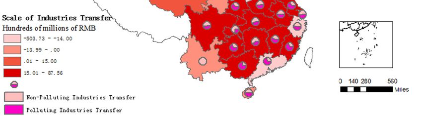
Int. J. Environ. Res. Public Health 2019, 16, 423                                                 2 of 27

pollution prevention and control were proposed, in which Article 5 involved strict energy
conservation and environmental protection measures, optimization of the layout of industrial space,
strengthening of environmental supervision and the prohibition of the transfer of outdated
production methods [13].
      To optimize industrial layout, in 2012 the Ministry of Industry and Information Technology
released the “Guidance Catalogue on Industrial Transfer,” which established an industrial
development pattern featuring “one axis, one belt, five circles and five groups.” It also involved the
industries in the coastal areas shifting to the central and western regions, with the central region also
adopting staged development strategies to actively undertake industrial transfer from the eastern
region. As a strategic decision in China’s industrial policy, industrial transfer not only promotes the
transformation and upgrading of China’s industry, but also is an important practice to optimize the
spatial layout of industry [14]. Some industrial transfer achievements have already been made [15],
and the spatial layout of industry has gradually become clear in the Beijing-Tianjin-Hebei region,
which not only specifically explains the non-capital function of Beijing, but also has played an
important role in driving industrial transformation and the upgrading of neighboring provinces and
cities. By focusing on electronic information, precision equipment, automobiles, household
appliances, and clothing and textiles, the Yangtze River Economic Belt has undergone industrial
transfer and clustering to develop an industrial spatial layout that is compatible with the carrying
capacity of resources and the environment. In 2016, the industrial added-value of the Yangtze River
Economic Belt was RMB 97,835.33 billion and regional production totaled RMB 259,941.66 billion,
increasing by 59.87 and 85.5% (calculated at flexible prices), respectively, compared to 2010 values.
Industrial transfer has led to rapid economic development in adjacent areas, the upgrading of
industrial structure in the receiving area, and the optimization of industrial spatial layout. However,
it is still unknown whether the spatial optimization of industrial areas brought about by industrial
transfer can alleviate haze pollution.
      Most studies of the effect of regional industrial transfer have focused on economic effects or the
effects of technology spillover [16,17], while the environmental effects of regional industrial transfer
remain controversial. For example, industrial transfer in the Beijing-Tianjin-Hebei region does not
exacerbate environmental pollution in the region [18], while industrial transfer in the central region
is accompanied by pollution leakage [19]. Industrial transfer has been extended from the pilot areas
to the national level; however, studies of the regional environmental effects not only lack a
consideration of the overall process, have also not accurately measured the environmental impacts
of industrial transfer on the receiving areas. To objectively evaluate the impact of regional industrial
transfer on haze pollution in China, and propose an economic method to control haze pollution from
the perspective of industrial transfer, 30 provinces in China from 2008 to 2016 were used as samples.
The study adopted the spatial panel model to analyze the haze pollution effects of industrial transfer
based on the spatial spillover of haze pollution.
      The remainder of the paper is organized as follows: Section 2 reviews the previous related
studies. The research methods and data are described in Section 3. The empirical results are presented
and discussed in Section 4. Finally, we conclude our study in Section 5.

2. Literature Review
     Both international and regional industrial transfer can generate adverse environmental effects
and have been considered in previous studies. The status of international industrial transfer is usually
measured in terms of foreign direct investment (FDI), but a consensus on the environmental effects
of FDI is yet to be reached. The pollution haven and pollution halo hypotheses have been proposed.
Copeland and Taylor [20] first proposed the pollution haven hypothesis based on a study of the
relationship between northern and southern trade and the environment. According to the hypothesis,
the free flow of production factors encourages pollution-intensive industries to use FDI as a carrier
to transfer to countries with loose environmental regulations, and areas with lower environmental
regulation standards will then become a haven for polluting industries [21,22]. Subsequently, many
Chinese and international researchers have incorporated control variables such as economic growth,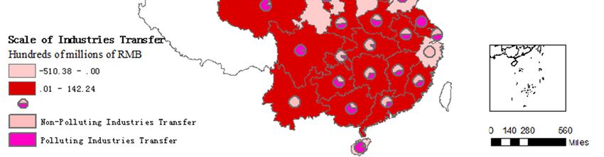
Int. J. Environ. Res. Public Health 2019, 16, 423                                                3 of 27

R&D level, energy consumption, and urbanization into their research to verify the pollution haven
hypothesis and estimate the impact of FDI on environmental pollution. However, some researchers
hold the opposite view and believe that FDI improves the environmental quality of host countries
through economic growth and the introduction of high level technologies. For example, when Liang
[23] explored the relationship between urban air pollution, industrial structure, and FDI in China, a
significant negative correlation between FDI and air pollution was discovered, with FDI deemed to
be beneficial to the environment of the host country. Deng and Xu [24] used a spatial lag model (SLM)
and a spatial error model (SEM) to analyze the relationship between FDI and environmental pollution
in various provinces in China during 2000-2009, and concluded that the pollution haven hypothesis
was not established, with FDI significantly easing China’s environmental pollution. In some studies,
the two viewpoints expressed above have been combined. For example, Liu et al. [25] used an SLM
and SEM to analyze the impact of China’s FDI inflow on different types of environmental pollution
and discovered that the impact of FDI was significantly different for different types of environmental
pollution. This confirmed the existence of both the pollution haven and pollution halo hypotheses.
     There are fewer studies of the impact of regional industrial transfer on the environment than the
environmental effects of international industrial transfer. Zheng et al. [26] analyzed the water
pollution status in industrial export areas and areas undertaking various industrial activities, and
discovered that industrial transfer of electronics, plastics and bio-pharmaceutics caused the transfer
of water pollution. Lin and Zou [27] employed the ACT model to test the environmental effects of
China’s regional industrial transfer based on data from 2000 to 2011, and found that industrial
transfer between the east and the west has accelerated the transfer of pollution. Zhang and Gou [28]
analyzed Chinese provincial data and found that the transfer of polluting industries has accelerated
the pace of environmental pollution in underdeveloped areas; however, it was concluded that
targeted environmental regulations would generate a win-win result for the environment and the
economy. Dou and Shen [19] explored the environmental impact of pollution-intensive industries in
central China, and found that the transfer of polluting industry has led to the transfer of pollutants
such as wastewater, SO2 and soot to the central region. Xu et al. [29] studied the relationship between
regional industrial transfer and carbon transfer in China, and found that the relationship between
industrial transfer and carbon transfer had an “inverted U” shape. Although not all provinces had
exceeded the turning point, industrial transfer had increased the transfer of carbon emissions.
     There are two main categories of research on haze pollution, i.e., studies of the components and
major influencing factors of haze, and studies of solutions to haze pollution. The main components
of haze are SO2, NO2, and inhalable particulate matter, in which the inhalable particles when
combined with fog will become haze. Natural factors are only part of the cause of haze pollution,
while socio-economic factors are the root cause of serious haze pollution in China. Haze is mainly a
consequence of the lack of development of new energy technologies, with coal remaining as the main
energy source, a high proportion of heavy industry in the industrial mix, motor vehicles as the main
means of transportation and a large amount of dust generated by construction sites as urbanization
proceeds. Further studies have shown that factors such as fiscal decentralization, energy price
distortion, and environmental regulation are positively related to haze pollution, while industrial
clustering will effectively alleviate the degree of haze pollution. The government is currently mainly
focused on economic solutions to vigorously control haze, including taxation policies based on a
resource tax [30], sulfur tax [31], and carbon tax [32,33]. Other countermeasures are also proposed,
such as improving the system of atmospheric emission rights trading, perfecting the laws and
regulations in place for haze management, and building a regional haze joint prevention and control
mechanism.
     Some studies have suggested that industrial transfer will have an impact on the status of haze
pollution in each province. Leng et al. [34] analyzed data for China’s provinces and confirmed that
FDI is positively related to haze pollution in China; however, Li et al. [35] undertook a case study of
the Pearl River Delta and showed that FDI can effectively alleviate the severity of haze pollution in
the region. The study was conducted from the perspective of international industrial transfer, while
research on the impact of regional industrial transfer on haze pollution is still limited. Industries in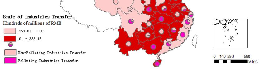
Int. J. Environ. Res. Public Health 2019, 16, 423                                                   4 of 27

China’s developed regions are moving to underdeveloped regions in an orderly manner. To prevent
the underdeveloped regions from continuing to adhere to the old policy of “pollution first and
treatment later”, this study explored the relationship between regional industrial transfer and haze
pollution in China. It can provide suggestions for the management of haze from the perspective of
industrial transfer.
     There are defects in existing studies of the effect of national industrial transfer on haze pollution,
and there is a need to accurately evaluate the impact of regional industrial transfer on haze pollution.
Apart from previous research, this study extends them from the following perspectives: (1)
Compared with the research on the issue of international industrial transfer, there are few studies on
the environmental pollution caused by industrial transfer at provincial level. It is urgent to study the
impact of domestic industrial transfer on haze pollution, especially at the time that the main way to
alleviate haze pollution in China is industrial transfer. (2) Based on the deviation-share method and
entropy weight method, the industrial transfer index was constructed, which not only excludes the
influence of time factor and technological progress, but also takes the policy factor into consideration.
(3) We examined the impacts of industrial transfer on haze pollution from the perspectives of level
and scale respectively. Moreover, industrial areas were distinguished as undertaking zones and
transferring zones. (4) We divided the secondary industry into polluting industry and non-polluting
industry, and explored the impact of different industrial types on haze pollution. It will provide
relevant suggestions for the central and western regions to undertake proper transferring industry.

3. Methodology and Data

3.1. Methodology
      Cross-regional industrial transfer can result in macro-level industrial restructuring and changes
of regional industrial distribution, and its impact on environmental quality should be paid attention
to seriously. This is particularly the case for the increasingly serious incidences of air pollution in
China, with haze pollution posing serious risks to public health and causing huge economic losses.
As industries move among provinces, industrial transfer from a certain province may affect the haze
pollution of others. In this study, the impact of industrial transfer on the haze pollution in each
province was considered, but it was recognized that ignoring the spatial effects associated with
would cause the model to be set incorrectly. Therefore, a spatial econometric model was used to
investigate the relationship between industrial transfer and haze pollution, and to measure the spatial
spillover effects of various influencing factors.
      As spatial econometric analysis technology develops, the most widely used models have
changed from spatial auto-regression (SAR) model and spatial error model (SEM) to spatial
interaction models (i.e., the spatial Dubin model: SDM) and spatial auto-correlation (SAC) models.
The transmission mechanisms and economic implications vary among the different types of models.
Containing only the dependent variable lag term, the SAR models assume that the dependent
variable will affect haze pollution in other areas through spatial interaction [36]. SEM only contain
the spatial auto-correlative error term, with the spatial spillover effect considered a random impact,
enabling errors to be transmitted as a result. Both the SDM and the SAC model contain a dependent
variable lag term and a spatial auto-correlative error term, with the two spatial effect conduction
mechanisms also taken into consideration. In addition, the SDM includes a spatial interaction,
meaning that the haze pollution in a certain province is not only affected by a series of local
independent variables, but also by the haze pollution of other provinces and its independent
variables [37]. Because the setting of a spatial econometric model is key to revealing the correlation
between variables, for a better model fitting, this study used the ordinary least squares (OLS)-
[SAR\SEM]-SAC-SDM concept in modeling and the Lagrange multiplier statistic, Wald statistic, and
likelihood ratio (LR) to test the effectiveness of model fitting. Due to the existence of a spatial lag
dependent variable and lag error variable, it could not be assumed that the strict exogenous and
residual perturbation terms of the explanatory variables are independent and identically distributed
as in a traditional econometric model.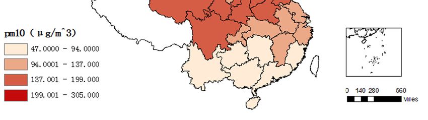
Int. J. Environ. Res. Public Health 2019, 16, 423                                                     5 of 27

     The spatial dependence of economic variables is taken into account in the construction of a
spatial econometric model, and it could be compared with a traditional econometric model. It could
not be assumed that the strict exogenous and residual disturbance terms of the explanatory variable
in the traditional measurement model are independent and identically distributed because of the
existence of a spatial lag variable and lag error variable. Methods such as the instrumental variable
method [38–42] or maximum likelihood estimation method [43–46] need to be selected for model
estimation. Because it is very difficult for the instrumental variables (IV) method to select suitable
variable tools, and its parameter estimation results tend to exceed the domain, a maximum likelihood
estimation (MLE) was employed to estimate the model and avoid the problems described above.
     The following models were constructed based on the information given above:
                       =      +              +            +                    +          +       +      (1)

                                            =        +            +            +              +
                                                                                                         (2)
                                        =             +
     Equation (1) is the SDM, while Equation (2) is a SAC model. Partial constraints were added to
these models before obtaining SAR, SEM, and OLS models.
     If the spatial interactions examined in the SDM do not exist, the SDM is transformed into an SAC
model. In addition, when the spatial auto-correlative error term coefficient in the spatial crossover
model is zero, the model is transformed into the SAR model, e.g., Equation (3):
                                            =        +            +            +              +          (3)
   When       +     = 0 is obtained in the SDM, or when the spatial lag term coefficient in the SAC
model is zero, the model is transformed into an SEM, e.g., Equation (4):
                                                     =    +               +           +
                                                                                                         (4)
                                                 =         +
    When spatial correlation is not considered in the model, it is transformed into an OLS model,
with all spatial correlation coefficients being zero, e.g., Equation (5):
                                                     =    +               +           +                  (5)
     Here, Yit is the annual average PM10 concentration in the provinces in year t; Xit is the core
explanatory variable-industry transfer, and the detailed measurement method is as follows. The
industrial transfer status of each province was measured from multiple dimensions, and the
corresponding model was built for an analysis of the industrial transfer level (IT), non-polluting
industry transfer level (ITN), polluting industry transfer level (ITP), the scale of industrial transfer
(SIT), the scale of non-polluting industry transfer (SITN), and the scale of polluting industry transfer
(SITP). Xcontrol refers to a series of control variables, including population density, GDP per capita,
street lighting brightness, energy mix, vehicle use, environmental regulations, industrial structure,
rainfall and humidity. μit and εit are random disturbances subject to a normal distribution; W is a
spatial weighting matrix, with elements generally determined in terms of the spatial unit’s
connectivity. If the regions are adjacent the elements value is one, otherwise the value is zero. Because
the relationship between the regions cannot be fully reflected in the geographic adjacency matrix,
and the haze spillover effect is related to the distance between the two provinces, with a larger
distance between provinces, the spatial spillover effect of haze will be weakened. Therefore, the
spatial weighting matrix was constructed based on the gravity model:
                                                                          ∗
                                                                                , ≠
                                                              =                                          (6)
                                                                      0       , =
    Here, i and j represent each province;           is the average PM10 concentration in province i from
2008 to 2016; and dij is the linear distance to the geographical center of the province (km).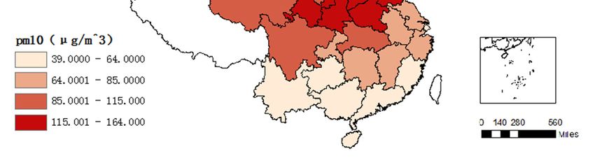
Int. J. Environ. Res. Public Health 2019, 16, 423                                                                6 of 27

3.2. Variables and Data

3.2.1. Interpreted Variable
     PM10 concentration. PM2.5 data has only been available in China since the end of 2012, and most
of the literature refers to the global average annual PM2.5 concentration published by the Center for
Social and Economic Data and Applications of Columbia University. The data covers the period from
1998 to 2012; however, the data are found to be of poor quality, with the only usable data covering
the period from 1999 to 2011. The focus of this study is the spatial spillover effect of industrial transfer
on haze pollution, but the available data do not cover the critical period of China’s industrial transfer.
There are gaps in the urban PM2.5 concentration data published by China’s environmental protection
departments for different major cities. Particulates are an important constituent of haze, but due to
the gaps in PM2.5 statistical data and the wide availability of PM10 concentration data, the PM10
concentration in provincial capitals (unit: μg/m3) was used as an indicator of the haze level in each
province [47].

3.2.2. Explanatory Variables
      Industrial transfer. The characteristics of industrial development influence the industrial transfer
process. The location of agriculture, extractive industries, and various service enterprises are related
to natural resource endowment and long-distance transportation. Industrial transfer occurs mostly
in industrial manufacturing, and the development of manufacturing enterprises can have a
significant impact on environmental pollution [48]. Therefore, this study focused on the impact of
industrial manufacturing transfer on haze governance in China. Industrial classification refers to the
Industrial Classification of the National Economy standard. Because of the differences in the
statistical yearbooks and the overall lack of data, the industries were integrated and divided into 20
categories to ensure data consistency and availability. The effect of industrial transfer on haze was
decomposed to distinguish between the transfer of polluting and non-polluting industries. Table 1
shows the details of this division.

                            Table 1. Classification of 20 industrial manufacturing industries.

  Classification        Number                                              Industry
                                         Processing of Food from Agricultural Products (1); Manufacture of Foods (2);
                                         Manufacture of Tobacco (3); Manufacture of Textile (4); Manufacture of
                                         General Purpose Machinery (5); Manufacture of Special Purpose Machinery
  Non-polluting
                             9           (6); Manufacture of Railway, Ship, Aerospace and Other Transport
    industry
                                         Equipments (7); Manufacture of Computers, Communication and Other
                                         Electronic Equipment (8); Manufacture of Measuring Instruments and
                                         Machinery (9)
                                         Manufacture of Liquor, Beverages and Refined Tea (10); Manufacture of Paper
                                         and Paper Products (11); Processing of Petroleum, Coking and Processing of
                                         Nuclear Fuel (12); Manufacture of Raw Chemical Materials and Chemical
     Pollution                           Products (13); Manufacture of Chemical Fibres (14); Manufacture of Non-
                            11
     industry                            metallic Mineral Products (15); Smelting and Pressing of Ferrous Metals (16);
                                         Smelting and Pressing of Non-ferrous Metals (17); Manufacture of Metal
                                         Products (18); Manufacture of Medicines (19); Manufacture of Electrical
                                         Machinery and Apparatus (20)
     Based on the shift-share method, changes in the economic output of an industry over a certain
period of time can be decomposed into growth components at different regional levels to observe the
evolution of spatial and temporal trends, and the absolute scale of inter-regional industrial transfer:

                                                                 ,                       ,           ,
                                 ,   −    ,   =     ,   ∗            −1 +   ,   ∗            −                      (7)
                                                             ,                       ,           ,
Int. J. Environ. Res. Public Health 2019, 16, 423                                                                                 7 of 27

         ,   and     ,       refer to the total production value of time t and t-1 for industry k of province i,
                         ,
and      ,    ∗              −1   is the national growth component of the industrial scale. An increase in
                     ,

                                                                                                            ,           ,
province i, according to the national growth rate of industry k,                                ,   ∗           −           indicates the
                                                                                                        ,           ,
province’s growth component of the industrial scale. If the difference between the growth rate of
province i and the national growth rate is greater than zero, the province experiences an industrial
transfer; otherwise there is an industry transferred out of the province.
     To obtain comprehensive indicators of industrial transfer in each province, the weighting of
potential indicators was determined based on the principle of information entropy of data from the
transfers of 20 industries in each province. The following steps were used to process the data to
compare the comprehensive indicators of industrial transfer in different provinces for different years.
     First, the indicator was selected. Assuming there are z years, x provinces, and y industries
transferred, xtij indicates the transfer value of industry j in province i in year t.
     Second, the indicators were standardized. The original indicators were standardized by the
following formula to eliminate the influence of the dimension and unit difference between the
indicators on the results:

                                                                            ,
                                               Positive indicator:                   =                                                (8)

                                                                                ,
                                              Negative indicator:                       =                                             (9)

where,      ,     represent the maximum and minimum values, respectively, in the transfer of
industry j.
    Third, the weighting of the indicator was determined by the principle of information entropy:
                                                                        ,
                                                             =                      ,                                                (10)
                                                                 ∑ ∑

      Fourth, the entropy value of the jth indicator was calculated:

                                                     =−                             ∗ Ln(   )                                        (11)

where        =     ( × ).
      Fifth, the information utility of indicator j was calculated:
                                                              =1−                                                                    (12)
      Sixth, the weightings of each indicator were calculated:

                                                                =                                                                    (13)
                                                                    ∑

     Finally, the level and scale of industrial transfer in each province were calculated. Using the
weighted coefficient wj, the weighted summation of each industry transfer index was calculated, with
the result representing the level and scale of industrial transfer in each province:

                                                            =                                                                        (14)

                                                            =                                                                        (15)

     Based on the above, the variables IT, ITN and ITP were obtained to measure the industrial transfer
level of each province, while the variables SIT SITN, and SITP were obtained to measure the scale of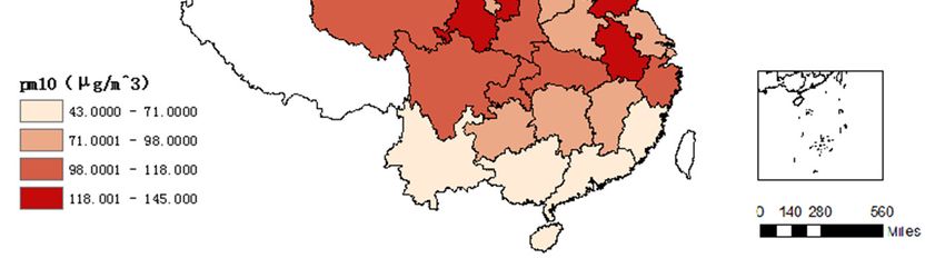
Int. J. Environ. Res. Public Health 2019, 16, 423                                                                   8 of 27

industrial transfer in each province, with a positive direction indicating an inbound industrial
transfer and a negative direction indicating an outbound industrial transfer.

3.2.3. Control Variables
      Population size. Because of the large differences in the administrative area and population size of
each province, there is no comparability in terms of the absolute value of population size. Hence,
Shao et al. [49] adopted a population density measurement, i.e., the ratio between the total population
and administrative area of each province (unit: persons per km2) to measure the influence of
provincial population agglomeration on local haze pollution.
      Level of economic development. According to Kuznet’s hypothesis, the regional economic level has
an impact on the local environmental quality. Therefore, this study included the economic
development level as a variable. It was measured by per capita GDP (yuan/person) and street
lightness intensity. From the availability of data, street lightness was measured by adopting the
logarithm of the urban roadside lighting level provided by the Bureau of Statistics.
      Energy mix. Fossil energy burning is the main cause of haze pollution, especially the burning of
coal [50–52]. Because the main energy source in China is coal [53], energy mix is represented by the
ratio of coal consumption to total energy consumption [54].
      Vehicle use. The mileage of motor vehicles and local pollution levels are closely related. Vehicle
exhaust emissions are not only a direct source of PM10, but also are the main source of secondary PM10.
Some studies have reported that motor vehicle exhaust is the main source of PM10 in the urban
atmosphere [55,56]. The ratio of highway mileage to the administrative area in each province was
employed in this study to indicate the local vehicle use.
      Level of environmental regulation. Environmental regulation by local government aims to alleviate
the pressure of environmental pollution. According to some studies, intense environmental
regulation has alleviated the pressure of local haze pollution. However, other studies have shown
that the effect of environmental regulation on haze pollution is not satisfactory [57,58]. The promotion
of official evaluation systems centered on gross national production has resulted in environmental
regulatory behavior being imitated among provinces and regions, thus further degrading the
environmental quality [59]. This study measured the intensity of local environmental regulation
through a ratio of industrial pollution control investment and industrial added value in various
regions.
      Industrial structure. The degree of haze pollution can be enhanced by the development of
secondary industrial sources, for example, exhaust emissions from burning fossil fuels and
suspended dust caused by the development of the real estate industry. Industrial development
consumes large amounts of energy, and industrial emissions directly increase the degree of haze
pollution [60]. The industrial structure of each province was measured by the ratio of the industrial
added value of each province to the gross national product.
      Table 2 presents the definitions and abbreviations for these variables in the text.

                                                    Table 2. Definition of variables.

  Variables           Symbol                            Variable                                Definition
 Explanatory                                                                            Annual PM10 Concentration in
                          Y                    PM10 Concentration
  Variable                                                                                   Provincial Cities
                          IT          Industrial transfer level
                         SIT          Industrial transfer scale
                                      Non-polluting Industrial transfer
    Core                 ITN                                                      Based on the shift-share method and
                                      level
 explanatory                                                                      entropy weight method, and the specific
                                      Non-polluting industrial transfer
   variable              SITN                                                     calculation steps are shown above
                                      Scale
                          ITP         Polluting Industrial transfer level
                         SITP         Polluting industrial transfer Scale
    Control              POP          Population size.                            Total population/administrative area
    variable           RGDP           Per capita GDP                              GDP/total population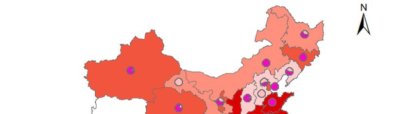
Int. J. Environ. Res. Public Health 2019, 16, 423                                                                   9 of 27

                          SL          Stable lighting brightness              The logarithm of city road lighting
                                                                              Coal consumption/total energy
                         EM           Energy mix
                                                                              consumption (standard coal)
                       ROAD           Vehicle use                             Highway mileage/administrative area
                                                                              Industrial pollution control investment
                          ER          Level of environmental regulation
                                                                              /industrial added value
                         SEC          Industrial structure                    Industrial added value/GDP
                        RAIN          Rainfall capacity                       Average annual rainfall
                                                                              Absolute humidity/saturated absolute
                    HUMIDITY          Relative humidity
                                                                              humidity
     Meteorological conditions. Meteorological conditions are also a significant factor affecting the
degree of haze pollution. In 2017, the National People’s Congress proposed that great importance
should be attached to the impact of relative humidity on haze pollution. In this study, the
precipitation (unit: mm) and relative humidity of each region were used to measure local
meteorological conditions.

3.2.4. Sample Selection and Data Sources
     Samples were collected for 30 provinces in China from 2008 to 2016. Tibet, Hong Kong, Macao,
and Taiwan were excluded due to the availability of sample data. PM10 concentrations were obtained
from the China Environmental Statistical Yearbook, raw industrial transfer data were collected from
the China Industrial Statistical Yearbook, coal consumption and energy consumption (standard coal)
data came from the China Energy Statistical Yearbook, and other data were sourced from the China
Statistical Yearbook.

3.3. Descriptive Statistics of Variables
      Descriptive statistics for the variables are provided in Table 3. There have been remarkable
advances in the prevention and control of China’s haze pollution in recent years, although the
average annual PM10 concentration remained seriously high at 101.11 μg/m3. The atmospheric quality
of Hainan Province has been maintained well, with an annual PM10 concentration of only 34 μg/m3
at its lowest, but in 2013, the annual PM10 concentration in Hebei Province reached 305 μg/m3. To
effectively alleviate the haze pollution situation, the “Ten Articles of Atmosphere” clearly identified
that the elimination of outdated production methods will force industrial transformation and
upgrades, and it is strictly prohibited to transfer outdated production methods and heavily polluting
industry. This plan has achieved considerable results so far. The output value of China’s industrial
manufacturing industry has shown an overall downward trend, while the output value of non-
polluting industries has remained basically stable, but the output value of polluting industries has
declined dramatically. Energy mix and industrial structure are the main factors influencing levels of
haze pollution. China’s energy consumption structure is dominated by coal, with an average coal
consumption ratio as high as 74.741%. The top three provinces in the country in terms of coal
consumption are Shanxi, Inner Mongolia, and Guizhou, with an average coal consumption ratio of
91.99%. With the transformation and upgrading of industrial structure in China, the proportion of
industrial production occurring in secondary industries in each province has presented the trend of
a year-on-year decrease.

                                       Table 3. Descriptive statistics for the variables.

          Variables                        Mean                Std. dev.                Min                 Max
              Y                            101.11                31.99                   34                  305
              IT                           0.652                 0.140                 0.415                1.484
            SIT                           −17.111               290.037               −4561.08             333.177
             ITN                           0.639                 0.148                 0.405                1.431
            SITN                           0.004                38.969                −257.151             147.557
             ITP                           0.662                 0.150                 0.423                1.817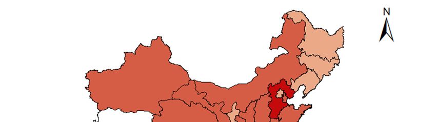
Int. J. Environ. Res. Public Health 2019, 16, 423                                               10 of 27

            SITP                          −17.115    281.681           −4552.76            285.445
            POP                           2791.789   1214.515            649                 5967
           RGDP                           42675.15   22442.85            9855              118198
             SL                            13.159     0.742             11.086              15.068
            EM                             74.741     13.038            29.119              93.710
          ROAD                             13.814     23.167            0.083              125.397
             ER                            3.745      3.329             0.359               28.039
            SEC                            39.691     8.230             11.904              53.036
           RAIN                           950.842    569.967            148.8               2939.7
         HUMIDITY                          65.878     10.461              42                  85

3.4. Framework of This Research
      The overall framework of this study is presented in Figure 1. Based on the deficiency of previous
literature, this research adopted the deviation-share method and the principal component analysis
method to calculate the level and scale of industrial transfer in 30 provinces in China respectively. In
particular, the traditional econometric model and space panel model were used in this study.
Through Spatial Durbin Model, Spatial Auto-regression Model, Spatial Autocorrelation Model and
Spatial Error Model, as well as Ordinary Least Square Model, the effect of industrial transfer on haze
pollution is investigated. Taking into account the development gaps between different regions, China
is divided into eastern, central and western regions to examine the environmental effect of industrial
transfer. Next, the spatial weight matrix in the model was be replaced for analysis and the robustness
of the benchmark model was tested. Finally, based on the empirical results, we summarized our
research and put forward some policies and suggestions.
Int. J. Environ. Res. Public Health 2019, 16, 423 11 of 27
1. Introduction 2. Literature review 3. Methodology and data
Literature review Methodology (OLS and spatial
economics models)and
Background and
Gaps Statistics for Variables
research aims
(Spatial correlation tests,
Contributions descriptive statistics)
4. Results and discussion Analysis models
OLS SEM SAR
SDM SAC
Research sample
Total transfer industries
Non-polluting industries
Polluting industries 1) Estimates of both
OLS models and spatial
Economics models
Model check
Robustness tests
Hausman tests
Conclusions and
policy implications
Replace the space weight matrix Wald tests
LR tests
5. Conclusions and
2) Robustness tests
policy implications
Figure 1. Framework of this research.
4. Results and Discussion
4.1. Variation Trend of Industrial Transfer and Haze Pollution
The “Environmental Air Quality Standard-GB 3075-2012” was promulgated and implemented
in early 2016. It divides atmospheric environmental quality into two grades according to the annual
PM10 concentration, and removes the third level standard. The first grade PM10 annual concentration
limit is 40 μg/m3 and the second grade is 70 μg/m3. Due to the large time period considered in this
study, the classification of the atmospheric environment used the previous Ambient Air Quality
Standard-GB 3095-1996, which has an average annual first grade limit of 40 μg/m3, second grade limit
of 100 μg/m3, and a third grade limit of 150 μg/m3.
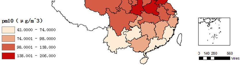
As shown in Figure 2, among all the provinces and regions investigated in this study only
Hainan Province had air quality at the first grade with respect to PM10. The implementation of the
“Ten Articles of Atmosphere” has effectively alleviated haze pollution in China. In 2016, the PM10
concentration in Beijing was 16 μg/m3 lower than in 2013. Air quality in most of the central and
eastern provinces, as represented by Hubei, Anhui, Jiangsu, Heilongjiang, Jilin, and Liaoning, has
improved significantly, and the quality of the atmospheric environment has reached the second grade.
Haze pollution in Qinghai, Gansu, Shaanxi, Henan, and Shandong has also been effectively alleviated.Int. J. Environ. Res. Public Health 2019, 16, 423 12 of 27
The quality of the atmospheric environment is stable within the limits of the third grade. As of 2016,
the atmospheric environmental quality of Hebei Province still exceeded the third grade limit, but it
had decreased by 46.2% compared to the average annual PM10 concentration in 2013. Although the
reduction is remarkable, there is still a need for further prevention and control of haze pollution in
Hebei Province.
(a) 2008
(b) 2013Int. J. Environ. Res. Public Health 2019, 16, 423 13 of 27
(c) 2014
(d) 2016
Figure 2. Variation trend of PM10 average concentration in each province: (a) 2008, (b) 2013, (c) 2014, (d) 2016.
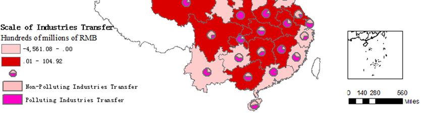
Figure 3 shows that China’s industrial manufacturing industry has displayed a trend to shift
toward the central and western regions between 2008 and 2016. Compared with the western
provinces, the central region has a high industrial transfer competitiveness, and is the main location
for the transfer of industrial manufacturing from the eastern regions. Most of the central and western
provinces have a relatively high proportion of polluting industries that could be transferred. For
example, Xinjiang, Jilin, and Qinghai account for more than 80% of the transfer of polluting industries,
with high-end industries still concentrated in the eastern region. The areas of industrial transfer are
mainly concentrated in administrative districts such as Beijing, Shanghai, Hebei, Zhejiang, Liaoning,
and Guangdong provinces, accounting for 95% of the total transferred volume. In addition to the
eastern provinces, a small number of western provinces (e.g., Gansu, Inner Mongolia, Ningxia, and
Heilongjiang) have also experienced small-scale outgoing industrial transfers.
(a) 2008Int. J. Environ. Res. Public Health 2019, 16, 423 14 of 27
(b) 2012
(c) 2016
(d) 2008 to 2016
Figure 3. Spatial and temporal evolution of Chinese industry transfer: (a) 2008, (b) 2012, (c) 2016, (d)
2008 to 2016.
4.2. Impact of Industrial Transfer on Haze PollutionInt. J. Environ. Res. Public Health 2019, 16, 423 15 of 27
Based on the model settings described above, an OLS analysis of the impact of the overall
industrial transfer status on the haze pollution of each province was conducted, with the results
shown in Table 4. The spatial relativity of the model residuals was then analyzed.
Table 4. OLS analysis estimation results.
Explanatory
IT SIT POP RGDP SL EM ROAD ER SEC RAIN HUMIDITY R−sq
Variables
0.104 0.0696 0.174 −0.330
0.193 0.0231 0.117 0.0215 −0.0227 −0.0453
Model (1) *** ** ** *** 0.510
(1.56) (0.59) (1.32) (1.37) (−0.98) (−0.27)
(2.83) (2.47) (2.12) (−8.07)
0.100 0.0906 0.181 −0.330
0.00702 0.0205 0.0809 0.0256 −0.0229 −0.0778
Model (2) *** *** ** *** 0.510
(1.57) (0.52) (0.91) (1.61) (−0.99) (−0.45)
(2.73) (3.58) (2.20) (−8.08)
Note: t statistic values are shown in brackets; ** and *** mean p < 0.05 and 0.01 respectively.
The regression results presented in Table 4 show that the overall industrial transfer level and
scale have no significant effect on haze pollution. However, as shown in Figure 4, the OLS regression
residuals has a significant spatial correlation, and therefore, the OLS analysis could not objectively
display the relationship between variables. To improve the accuracy of the estimation, spatial panel
measurements were employed in the analysis and the spatial correlations between provinces were
taken into consideration. Prior to the spatial panel model regression, a spatial correlation test of the
dependent variable lnPM10 was conducted, with the test results showing a significant spatial
correlation (see Table 5).
0.25 0.2 0.188***
0.179***
0.2 0.179***
0.15
0.191*** 0.108***
0.146***
Morans’ I
Morans’ I
0.15 0.098***
0.113*** 0.15*** 0.1
0.1 0.117*** 0.102*** 0.102*** 0.103*** 0.107***
0.113***
0.098***
0.091*** 0.087***
0.05
0.05
0 0
2008 2010 2012 2014 2016 2008 2010 2012 2014 2016
Model (1) Model (2)
Figure 4. Identification for spatial correlation of OLS estimation error. Note: *** mean p < 0.01.
Table 5. Global Morans’ I indicators for PM10 in 30 provinces in China during 2008–2016.
Year Morans’I E (I) Sd (I) z p-value
2008 0.079 -0.033 0.047 2.406 0.008
2009 0.151 -0.033 0.047 3.953 0.000
2010 0.128 -0.033 0.047 3.457 0.000
2011 0.109 -0.033 0.046 3.074 0.001
2012 0.114 -0.033 0.046 3.181 0.001
2013 0.226 -0.033 0.045 5.788 0.000
2014 0.289 -0.033 0.047 6.292 0.000
2015 0.259 -0.033 0.047 6.256 0.000
2016 0.303 -0.033 0.047 7.180 0.000
Note: E (I) is the expected value of I; E(I) = −1⁄( − 1); Sd (I) is the variance of I; z is the z test value
of I; P is the probability.Int. J. Environ. Res. Public Health 2019, 16, 423 16 of 27
To explore the relationship between the overall industrial manufacturing transfer and haze
pollution, the overall industrial transfer level and scale were adopted respectively. The SEM, SAR,
SAC, and SDM were used in the analysis. A Hausman test was used to select the fixed effect spatial
panel model (Taking the SDM as an example to explore the effect of industrial transfer on smog
pollution, i.e., model (6), a Hausman test produced: chi2 (10) = 227.82, with a p value of 0.0000. When
the effect of transfer scale on smog pollution was considered, i.e., model (10), a Hausman test
produced: chi2(10) = 184.15, with a p value of 0.0000. The original hypothesis was rejected in both
cases and the fixed effect model was selected.), with the results shown in Table 6.
Table 6. Regression results of the impact of overall industrial transfer on haze pollution.
Overall Industrial Transfer Level Overall Industrial Transfer Scale
Explanatory SEM SAR SAC SDM SEM SAR SAC SDM
Variables Model Model Model Model Model Model Model Model
(3) (4) (5) (6) (7) (8) (9) (10)
0.186 0.300 * 0.343 ** 0.300 * 0.175 0.300 * 0.346 ** 0.300 *
δ or λ
(1.03) (1.66) (1.99) (1.67) (0.96) (1.66) (2.01) (1.67)
0.265 ** 0.263 ** 0.264 ** 0.209 **
IT
(2.26) (2.21) (2.26) (2.09)
0.00548 0.00562 0.00564 0.00612 *
SIT
(1.34) (1.36) (1.39) (1.85)
0.073 ** 0.0742 ** 0.0745 ** 0.181 *** 0.0647 ** 0.0663 ** 0.0666 ** 0.189 ***
POP
(2.33) (2.35) (2.38) (5.11) (2.08) (2.11) (2.13) (5.35)
−0.0717 −0.0740 −0.0739 −0.0352 −0.0834 −0.0856 −0.0855 −0.0390
RGDP
(−1.29) (−1.31) (−1.34) (−0.76) (−1.49) (−1.52) (−1.54) (−0.85)
0.0497 * 0.0501 * 0.0496 * −0.0386 0.0763 *** 0.0769 *** 0.0763 *** −0.0105
SL
(1.91) (1.92) (1.86) (−1.45) (3.14) (3.15) (3.07) (−0.41)
0.0538 0.0512 0.0515 0.195** 0.0118 0.00971 0.00992 0.174*
EM
(0.53) (0.50) (0.51) (2.13) (0.12) (0.09) (0.10) (1.93)
0.0262 * 0.0266 * 0.0269 * 0.045 *** 0.0320 ** 0.0322 ** 0.0325 ** 0.054 ***
ROAD
(1.87) (1.90) (1.93) (3.26) (2.29) (2.33) (2.35) (4.07)
−0.08 *** −0.08 *** −0.08 *** −0.0193 −0.082 *** −0.079 *** −0.079 *** −0.017
ER
(−3.70) (−3.49) (−3.52) (−0.99) (−3.66) (−3.47) (−3.50) (−0.88)
0.219 *** 0.222 *** 0.224 *** 0.368 *** 0.242 *** 0.244 *** 0.245 *** 0.343 ***
SEC
(2.71) (2.73) (2.73) (3.99) (3.01) (3.00) (3.01) (3.72)
−0.33* ** −0.32 *** −0.32 *** −0.25 *** −0.33 *** −0.32 *** −0.32 *** −0.26 ***
RAIN
(−8.13) (−7.80) (−7.98) (−6.09) (−8.06) (−7.74) (−7.92) (−6.27)
−0.171 −0.136 −0.139 0.654 *** −0.201 −0.166 −0.169 0.622 ***
HUMIDITY
(−1.06) (−0.83) (−0.87) (4.21) (−1.23) (−1.01) (−1.05) (4.02)
0.697
W×T
(0.96)
0.049 **
W×SIT
(2.06)
R2 0.733 0.743 0.744 0.885 0.724 0.735 0.736 0.885
Log−L 53.127 55.539 55.466 119.059 51.489 53.986 53.903 120.063
AIC −82.127 −87.078 −84.931 −194.12 −78.978 −83.972 −81.806 −196.126
BIC −39.073 −43.897 −38.152 −114.95 −35.797 −40.791 −35.027 −116.961
Year Yes Yes Yes Yes Yes Yes Yes Yes
Note: t statistic values are shown in brackets; *, ** and *** mean p < 0.1, 0.05 and 0.01 respectively.
Among models (3) - (10), a number of regression coefficients for SDM are significant in the fitting.
A Wald test and LR were used to further test the fitting effect of the SDM and the original hypothesisInt. J. Environ. Res. Public Health 2019, 16, 423 17 of 27
was rejected after considering the test result (When exploring the impact of the overall industrial
transfer level on smog pollution, the Wald test result is chi2 (10) = 38.86, with a p value of 0.0000; the
L ratio test statistical result is chi2(10) = 45.23, with a p value of 0.0000. When exploring the impact of
the overall industrial transfer scale on smog pollution, the Wald test result is chi2 (10) = 40.21, with a
p value of 0.0000; the L ratio test statistical result is chi2 (10) = 43.63, with a p value of 0.0000.). When
combined with the natural logarithmic values of each model, it is considered that the SDM has the
best fitting effect, i.e., the influence of the two spatial conduction mechanisms of haze pollution
contained in the SDM could not be ignored. Based on this, the SDM was selected for use in the
analysis.
The results in Table 6 show that, whether measured by the industrial transfer level or the
industrial transfer scale, the spatial lag coefficient is dramatically positive. This is further proof that
the haze pollution in China has obvious spatial agglomeration characteristics. Taking the results of
model (6) for example, every 1% increase in the PM10 concentration in a neighboring province will
contribute to a 0.3% increase across the region. Hence prevention and control of haze should be a
joint responsibility for the region. The leakage effect of haze pollution prevents unilateral haze
governance from achieving the desired results. Models (6) and (10) produce different values of the
independent coefficient, but the symbol and level of significance are basically consistent. The
influence of various factors is analyzed and is explained in the following paragraphs:
(1) Industrial transfer. The level and scale of industrial transfer are both positively related to haze
pollution. According to regional economic theory, industrial transfer not only promotes regional
economic integration, but also alleviates the problem of central city resources and environmental
pollution. Measured from either the level or scale of industrial transfer, the results of this study prove
that the transfer of industrial manufacturing makes haze pollution more severe in areas where
polluting industry is relocated too and to some extent alleviates the problem of industrial haze
pollution in the original location. As the main region of outbound industrial transfer, the eastern
developed areas have experienced an effective alleviation of haze pollution due to the large-scale
transfer of industrial manufacturing. However, the transfer of industrial manufacturing will slow
down the pace of local economic development. The transfer of secondary industry can effectively
alleviate the dependence of local economic development on these industries, promoting the
development of high tech industries, and forcing long term industrial transformation. This will not
only optimize the industrial structure and create new economic growth points, but will also
effectively alleviate regional environmental pressures.
Although haze pollution in areas where outbound industrial transfer is occurring can be
effectively alleviated due to the transfer of industrial manufacturing, from the national perspective,
industrial transfer cannot effectively control haze pollution, but would only enable its spatial
redistribution. With the environmental cost incurred by the eastern cities increasing annually, some
industrial manufacturing industries, especially polluting industries, have been actively shifting to the
central and western regions through the implementation of policies and government interests.
Central and western provinces are also actively promoting the transfer-in of eastern industries to
provide opportunities for development. China has a vast territory, but there is a serious imbalance in
the development of various regions. However, as China’s economy further develops, industrial
transformation and the upgrading of various provinces and regions are only a matter of time. The
central and western provinces have only considered economic development when undertaking
industrial transfer. An overreliance on industrial manufacturing, especially polluting industries, will
not achieve sustainable economic development. To alleviate the impact of polluting industries on the
quality of the local atmospheric environment, the government should undertake a comprehensive
consideration of the impact of enterprises on the regional economy and environment, encourage
enterprises to research and develop technologies for green production, and also provide
corresponding subsidies and preferential policies.
(2) Population density. Population density has a significant effect on haze pollution. Demand for
housing and transportation has increased as the population density has increased, which has directly
and indirectly exacerbated haze pollution in the region. With an ever-increasing population density,Int. J. Environ. Res. Public Health 2019, 16, 423 18 of 27
local haze pollution can be alleviated by improving the efficiency of urban resource utilization and
sharing facilities for pollution reduction. However, the positive externalities generated by population
concentration have yet to be fully utilized, which is also an issue that the government should consider
in future urban construction.
(3) Level of economic development. A negative correlation between the level of provincial economic
development and haze pollution is identified, but the relationship is not significant whether
measured from per capita GDP or lighting brightness (due to the possible multiple collinearity
problem, when measuring the level of economic development in terms of per capita GDP and lighting
brightness, a multi-collinearity test was conducted. The result is VIF = 2.89, indicating that there is no
significant multicollinearity.). Based on data from 1998 to 2012, Shao et al. [45] discovered that the
economic growth level and the haze pollution have a “U”-shaped relationship; some provinces have
already exceeded the inflection point and arrived at the stage where the economic growth level is
negatively related to haze pollution. Based on data from 2008 to 2016, it was found that the current
level of economic development does not have an obvious effect on haze pollution; in contrast, it could
alleviate the degree of local haze pollution. Although haze pollution is still persistent due to economic
development, the results indicate that China has entered the stage where haze pollution and
economic growth have become decoupled.
(4) Energy mix. Energy mix and haze pollution are positively correlated. Because China’s energy
mix is dominated by coal [61], pollutants such as soot and SO2 that are released from coal burning
are direct sources of haze. Coal accounts for as much as 70% of China’s energy consumption; however,
the growth in coal consumption has increased haze pollution. To alleviate the impact of excessive
coal consumption on haze pollution, the Chinese government should adopt policies such as actively
guiding people to use green energy, and adjust the national energy consumption structure to move
toward a green structure.
(5) Vehicle use. The local vehicle use is significantly positively correlated with the level of haze
pollution. Provinces with convenient transportation links and a developed road system will have
more motor vehicles and more exhaust gas emissions; hence, higher PM concentrations than
provinces with poor transportation. Transportation is one of the main factors influencing haze
pollution, and therefore the control of motor vehicle exhaust emissions would be an effective measure
to alleviate local haze pollution. The construction of a convenient public transportation system and
the widespread use of alternative energy vehicles would also be an effective means to alleviate haze
pollution.
(6) Level of environmental regulation. Results from other spatial measurement models have shown
that environmental regulation can significantly reduce haze pollution, but according to results gained
from the SDM, environmental regulation can alleviate haze pollution levels, although the effect is not
statistically significant. In this study, this variable was measured in various regions from the
perspective of the implementation of environmental regulations, and it was found that such
regulations do not fully meet their expectations. The investment output to alleviate industrial
pollution is insufficient, and it is necessary to increase investment in industrial pollution control by
the relevant government departments. Despite the insignificant effect of environmental regulations
on haze pollution, the role of environmental regulation in the control of haze pollution cannot be
ignored. Compared with remediation after the occurrence of haze pollution, it is better to prevent it
from happening. All provinces and autonomous regions should formulate corresponding
environmental protection regulations according to the local conditions, restrict the activity of
enterprises that emit large amounts of dust and polluting gases, implement effective pollution gas
emission standards, encourage cleaner production, enhance post-production supervision,
appropriately raise the penalty for defaulting, and ensure the sustainable development of enterprises
and regions.
(7) Industrial structure. The main factors causing haze pollution in China are the industrial
structure, which is based on the secondary industry, and the extensive industrial development model.
Some provinces still follow the development path of “pollution first and treatment later,” and the
promotion of GDP is still a key factor that encourages local governments to ignore environmentalYou can also read