BIS Working Papers What 31 provinces reveal about growth in China by Eeva Kerola and Benoît Mojon - Bank for ...
←
→
Page content transcription
If your browser does not render page correctly, please read the page content below
BIS Working Papers
No 925
What 31 provinces reveal
about growth in China
by Eeva Kerola and Benoît Mojon

Monetary and Economic Department

January 2021

JEL classification: C38, E01, E3, P2.

Keywords: China, GDP, provincial data, business cycles,
principal component.
BIS Working Papers are written by members of the Monetary and Economic
Department of the Bank for International Settlements, and from time to time by other
economists, and are published by the Bank. The papers are on subjects of topical
interest and are technical in character. The views expressed in them are those of their
authors and not necessarily the views of the BIS.

This publication is available on the BIS website (www.bis.org).

©   Bank for International Settlements 2021. All rights reserved. Brief excerpts may be
    reproduced or translated provided the source is stated.

ISSN 1020-0959 (print)
ISSN 1682-7678 (online)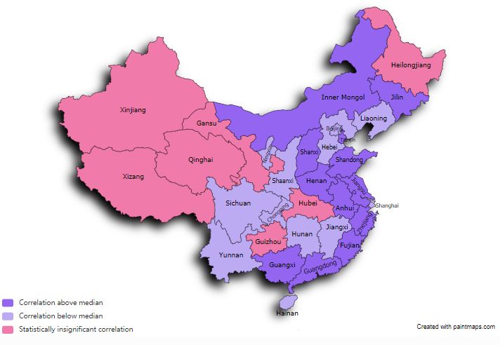
What 31 provinces reveal about growth in China
                                                Eeva Kerola*
                                               Benoît Mojon**

      Abstract
      It is important to understand the growth process under way in China. However, analyses of
      Chinese growth became increasingly more difficult after the real GDP doubling target was
      announced in 2012 and the official real GDP statistics lost their fluctuations. With a dataset
      covering 31 Chinese provinces from two decades, we have substantially more variation to
      work with. We find robust evidence that the richness of the provincial data provides
      information relevant to understand and project Chinese aggregates. Using this provincial
      data, we build an alternative indicator for Chinese growth that is able to reveal fluctuations
      not present in the official statistical series. Additionally, we concentrate on the determinants
      of Chinese growth and show how the drivers have gone through a substantial change over
      time both across economic variables and provinces. We introduce a method to understand
      the changing nature of Chinese growth that can be updated regularly using principal
      components derived from the provincial data.

* Senior Economist, Bank of Finland Institute for Emerging Economies (BOFIT)
** Head of Economic Analysis, Bank for International Settlements (BIS)

                                                        -1-
1. Introduction
The growth of the Chinese economy has been the main engine of the global economy over the last two decades.
Pre-Covid, new Chinese GDP accounted every year was larger than the US and the euro area new GDP combined.
China is now the second largest economy in the world, after the US and ahead of the euro area. Furthermore, a
major reason why emerging markets had a relatively smooth activity following the Great Financial Crisis owes to
a major infrastructure investment campaign in China which boosted the terms of trade for producers of
commodities.
However, the time series of Chinese growth is also among the most frustrating time series to date. Until the end
of 2019, it was desperately flat around 6%, mimicking the growth objective of the Chinese authorities. What is
flat offers little hope of any attempt of econometric analysis. In addition, even considering alternatives, such as
the famous Li Keqiang 1 index, offers only so much degrees of freedom to analyze the determinants of growth in
China.
In this article, we explore the time series of economic variables at the level of 31 Chinese provinces to gain insight
on the evolution and the determinants of economic activity in China. These data are published by the National
Bureau of Statistics (NBS), People’s Bank of China, China Ministry of Finance, Ministry of Human Resources
and Social Security and by a Chinese real estate website company SouFun-CREIS. Data is originally available
from 1999 at monthly, quarterly or annual frequency depending on the variable, but all series have been converted
to quarterly frequency. While there is no a priori reason that province level data are of a better quality than national
aggregate, we show that they do contain useful information to forecast Chinese economic activity. Their variance
is informative in this statistical sense. Our analysis using panel and time series approaches shows five striking
results.
First, province data help to project economic activity in China. Second, based on the province data we define a
new indicator of Chinese growth (The 31 Provinces China Business Cycle Indicator, or 31P-CBCI) that can pick
up fluctuations not present in the official data. It is updated quarterly as new provincial data becomes available
and published at the Bank of Finland BOFIT webpage 2. Third, the determinants of economic growth in China have
changed around 2010. Before, growth was driven by urbanization and productivity. Since 2010, growth is driven
by credit, house prices and public expenditure. In addition, urbanization has dragged on growth in this decade.
Fourth, the group of provinces pulling Chinese growth up has changed. The determinants of growth after 2010
apply more homogeneously to a larger group of Chinese provinces and those with the strongest correlation to
aggregate growth are now clustered across the coastal and central China. Five, we introduce a method to pinpoint
changes in the underlying determinants of Chinese growth that can be easily updated.
This paper contributes to two strands of literature. First, it gives new insights to the literature focusing on the
reliability of Chinese growth figures and measurement challenges of economic activity. The accuracy and
authenticity of Chinese official figures has been questioned by many for decades already. Appendix 1.1 in Jia
(2011) offers a thorough literature review on the studies of China’s macro-data quality. For the late 1990s and
early 2000s, Rawski (2001), Maddison and Wu (2006), Maddison (2006) and Young (2006) compare official GDP
1
Li Keqiang index was created by The Economist as an alternative measure for Chinese growth using three indicators (the
railway cargo volume, electricity consumption and bank loans) as reportedly preferred by the current Premier of China as
better economic indicators than official GDP numbers. Other alternative GDP measures include for ex. The Conference
Board’s Total Economy Database (Wu, 2014), Barclay’s index using PMIs, Bloomberg and Capital Economic indices using
linear combination of various economic variables, The Lombard Street Index, as well as different estimated economic
growth proxies as in Fernald et al. (2015) or Henderson et al. (2012).
2
www.bofit.fi/en/monitoring/statistics/china-statistics/ Direct link to data
-2-figures against various supply side indicators and find that the Chinese economy may have grown by a couple of
percentage points less than the official growth would suggest. There are studies that contradict these results and
find that the official data is roughly correct and may even understate the “true” economic growth (e.g. Holz, 2006a,
2006b, 2014; Clark et al., 2017a, 2017b; Perkins and Rawski, 2008). Further, it seems that information on different
business sentiment indicators (Mehrotra and Rautava, 2008) and various other economic indicators (Mehrotra and
Pääkkönen, 2011) convey useful information about developments in Chinese real economy.
Chinese official growth statistics started to raise more doubts again in the 2010s, after China explicitly announced
its ambitious decade-long real GDP doubling target in 2012. Following the announcement, real GDP growth rate
has been tracing its pre-announced annual targets to a frustrating degree losing practically all normal fluctuations.
As a result, several alternative GDP measures have emerged to better capture fluctuations in Chinese economic
growth.
Fernald et al. (2019) compose a China Cyclical Activity Tracker (China CAT) using a combination of eight non-
GDP indicators revealing fluctuations not present in the official growth rates. The Conference Board’s alternative
estimate for Chinese GDP (Wu, 2014) is constructed on a sector-by-sector basis, relying on both official and
constructed series. This GDP measure indicates larger volatility in the year-on-year estimates, sometimes showing
higher growth rates than the official numbers (de Vries and Erumban, 2017). After a US State Department memo
released by Wikileaks revealed that the current Chinese Premier, Li Keqiang, confided to the US ambassador in
2007 that to find out the true state of the economy, instead of the unreliable official GDP figures he himself turned
to electricity consumption, bank loans and railway cargo volume. Li was at the time serving as a party committee
secretary in the province of Liaoning. Also the Li Keqiang index reveals an economy much more volatile for the
recent years than what the official figures suggest. Other alternative indices include Barclay’s index, which uses
purchasing manager indices, as well as the Bloomberg and Capital Economic indices, which use linear
combinations of variables such as sectoral value added, freight, passenger traffic and retail sales. The Lombard
Street Index takes the official nominal GDP and a range of price indices covering all expenditure components and
calculates an alternative real GDP growth rate.
Chinese GDP growth has also been estimated using various techniques. Fernald et al. (2019) proxy China’s
economic activity with trade partner export data, whereas Henderson et al. (2012) turn to night-time light
intensities from satellite data that is immune to falsification and misreporting. Clark et al. (2017a and 2017b)
utilize this night-time light data to estimate an alternative weighted Li Keqiang-index. Kerola (2019) estimates
Chinese real GDP growth rates with alternative deflators using official price index data.
Our contribution to this debate is to provide an alternative business cycle indicator using only official provincial
macroeconomic data. Richness of the quarterly provincial data together with principal component analysis result
in a new indicator that is able to capture fluctuations in Chinese growth also for the more recent years.
Second, our paper also contributes to the strand of literature concentrating on understanding and analyzing the
determinants of Chinese growth. There are a number of structural factors in China that affect the growth process
under way: e.g. ongoing shift towards a more service-based economy, decreasing workforce, limits to internal
migration and ageing population. Greater awareness should be paid to the role played by structural transformations
in China as business cycle fluctuations still play a much smaller role (Laurenceson, 2013 and Laurenceson and
Rodgers, 2010).
As discussed with detail in Chen and Zha (2018), 1998 marked the beginning of the investment-driven phase in
China, where government effectively controlled aggregate bank loans by explicit M2 supply growth targets to
support investment especially in the heavy sector (e.g. infrastructure and real estate). The promotion of investment
at the sacrifice of consumption also meant that the relationship between investment and consumption broke down,
as the correlation between growth rates of investment and consumption changed from 0.80 to being statistically
-3-insignificant after 1998. Beginning of 2000s also marked the rise of China’s role in global trade flows. However,
as most of the investments were directed to the heavy, capital-intensive sector, they had little to do with increasing
exports that were mostly produced in the labour-intensive sectors.
Laurenceson (2013) finds evidence that demand shocks are a much greater source of output growth variance in
coastal provinces compared to inland provinces, which could be due to their greater exposure to international trade
and investments and are thus more affected by demand shocks originating from overseas. Démurger et al. (2002)
suggest that by the end of 1990s regions with similar geographical characteristics had converged, but inequality
between coastal and landlocked provinces persisted. Major factors preventing national convergence seem to be
inefficient capital allocation by the banking sector and low labour mobility. The eastern provinces grew faster also
because of high amounts of foreign investment. Poncet and Barthélemy (2008) analyse correlation of the provincial
data for 1991-2004 to see how synchronized business cycles are in China. Business cycles of the more remote
provinces show low correlations with the rest of the country as business cycles between two provinces are more
synchronized when production structures are more similar and labour can move more freely. Mehrotra et al. (2010)
find important differences in the inflation process across provinces using New Keynesian Phillips Curve to model
provincial inflation developments. What most explain these differences are the degree of development of the
market system and the relative exposure to excess demand pressures (GDP growth, labour productivity, level of
industrialization and migration). Gerlach-Kristen (2009) uses principal component analysis and finds evidence of
both business and inflation cycle synchronization across most Chinese provinces, apart from mainly the
northwestern provinces that have become less closely tied to developments in the rest of China.
Our contribution to this strand of literature is to use provincial data to show how the determinants of growth have
changed in China during the past two decades both with respect to economic variables and across provinces. We
show that during 1999-2010, aggregate growth was predominantly dependent on investments, internal migration
and productivity of the urban workforce. After 2010, growth has been increasingly dependent on government
expenditures, house prices and credit. We also show that after 2010, the new determinants of growth apply to a
much larger share of provinces and those with the highest correlation to aggregate growth are mainly situated in
coastal and central China. As an additional contribution, we introduce a simple method to pinpoint changes in the
underlying determinants of Chinese growth that can be updated regularly.
This paper is organized as follows. Section 2 discusses issues about Chinese economic data compilation and the
differences between national and provincial series. Section 3 introduces the provincial data used in more detail.
Section 4 presents the empirical analysis, including an alternative indicator for Chinese growth and a method to
reveal the changing nature of the growth determinants. Section 5 concludes.
2. National and provincial accounts
This section provides a short description of the Chinese economic data compilation and discusses the differences
between national and aggregated provincial series.
2.1. Data compilation
Before 1985, China’s national accounts were compiled according to the Material Production System developed in
the Soviet Union and used by countries with centrally planned economies. Gradually China moved to the United
Nations’ System of National Accounts (SNA). A more conventional value added approach was introduced in 1992.
China’s national GDP was initially estimated only from the production side, and the expenditure approach was
formally adopted by the National Bureau of Statistics (NBS) in 1993. Since 1992, both annual and quarterly
national GDP estimates have been published by the NBS. Currently China compiles its national accounts according
to the SNA 2008.
-4-At the central level, the NBS is responsible for organizing, directing and coordinating the statistical work
throughout the country. At the provincial level, the People’s governments at all levels and all departments,
enterprises and institutions may, according to the needs of their statistical work, set up statistics institutions (Vu,
2010). National GDP is compiled by NBS and (until very recently) gross provincial products (GPPs) were
compiled by provincial bureaus of statistics (PBS).
In principle, the national GDP should equal aggregated gross provincial product. However, there has been a large
discrepancy between the sum of Chinese GPPs and GDP, and the sum of GPP has been growing faster than the
national GDP. The main reason for the discrepancy is the use of enterprises as statistical units (and not
establishment) that can result in double counting. A local unit can be counted twice, first as part of the enterprise
at the place where the enterprise is located but where the activity does not take place and second also as a local
unit at the place where the activity takes place (Vu, 2010). Provinces also have incentives to exaggerate output
due to growth targets and the use of statistics to measure local policy makers’ achievements (Holz, 2014).
Data on enterprises whose output is above some cutting point are collected by surveys that are benchmarked on
the economic census data covering industrial, construction and service activities. Data on smaller enterprises are
estimated on the basis of administrative records like taxes. At the national level, administrative records on
nonmarket services can be used directly. However, to identify services at the local level, different surveys are used.
The same also occur to market services, surveys for the national level is carried out by the NBS and local bureaus
of statistics take care of the surveys at local levels (Vu, 2010).
Overall, the NBS has little control over provincial statistics bureaus or over the statistics divisions of other central
government departments and as a result most of the data compilation has occurred outside NBS control (Holz,
2014). Revelations during the last decade of some extensive data falsifications at the provincial level have caused
the NBS to rely more on economic censuses, annual data from directly reporting units, and sample surveys to
improve the accuracy of national figures. As a result, NBS took over the compilation of provincial gross product
totals from 2019 onwards and begun to develop a new system to generate and analyze national and provincial
balance sheets to improve the overall GDP compilation mechanism. Based on media reports, officials said the
move was part of the central government’s efforts to combat the discrepancies between provincial and national
figures, but the shift could also mean better inclusion of businesses not counted in statistics so far.
Since the NBS took over the compilation of provincial gross product totals, the provincial data was revised
extensively especially for 2018. Based on survey data the NBS revised downward the total provincial GDP of
2018 by 1 trillion yuan (140 billion euros). Largest cut was made in Tianjin province, where nearly 30% of the
provincial GDP was reduced. For some, annual GDP was increased, largest correction was boosting Yunnan’s
GDP of about 17%. All provincial data used in this paper are updated in 2020 and are thus based on the revised
series.
Overall, there is no reason to believe that provincial data would be of a better quality than the official national
aggregates. But as these recent large NBS data revisions suggest, measurement errors in provincial data can easily
occur in both directions. Moreover, while our data covers 11 economic variables for 31 provinces for 84 quarters
(altogether some 28,000 observations), there is sufficient grounds for treating possible measurement errors as
randomly distributed. Having substantially more variation to work with decreases the probability that the data
would as a whole deviate from the underlying true economic activity in one direction of another.
2.2. Nominal and real growth rates
Figure 1 presents Chinese nominal GDP growth rates, both the official, national series and the aggregated
provincial series. The series match to a high degree. For the provincial aggregate, growth peak before the great
-5-financial crisis dates a couple of quarters later than for the national growth and the economic recovery after the
downturn is much stronger. After 2012 however, these two series paint a fairly similar picture of the Chinese
economic development. This is not the case when looking at the real GDP series, as presented in Figure 2.
Apart from the obvious difference in the level of the real GDP growth rates, it is interesting that by aggregating
provincial real GDP figures one reveals fluctuations not present in the national series for the more recent years.
Especially after the China State Council explicitly announced the real GDP doubling target in 2012, the lack of
fluctuations in the national real GDP series is hard to ignore. The ambitious official goal was to double China’s
real 2010 GDP by 2020. This explicit growth target seems to have forced officials pursue numbers to meet their
mandated targets at many levels of the economy.
Figure 1: Nominal GDP growth rates in China: national and sum over provinces
Nominal GDP growth, Y/Y %
40
35
30
25
20
15
10
5
0
1998q1 2000q1 2002q1 2004q1 2006q1 2008q1 2010q1 2012q1 2014q1 2016q1 2018q1 2020q1
National growth Growth, sum over provinces
Figure 2: Real GDP growth rates in China: national and sum over provinces
Real GDP growth, Y/Y %
40
35
30
25
20
15
10
5
0
1998q1 2000q1 2002q1 2004q1 2006q1 2008q1 2010q1 2012q1 2014q1 2016q1 2018q1 2020q1
National growth Growth, sum over provinces
All in all, it seems more doubt has been cast on China’s real GDP figures than on nominal GDP numbers. Clark
et al. (2017b) note that there is much less discrepancy on average with nominal growth rates than between official
-6-central government and provincial real GDP growth assessments. They infer that the NBS computes the national
real GDP by taking the nominal growth rates reported by the provincial authorities and deflating them using a
common deflator.
China’s nominal GDP has also been subject to revisions as the NBS regularly conducts economic censuses that
may induce revisions to economic data. Holz (2014) documents that for example in the 2006 benchmark revision
following the 2004 economic census, the nominal value added for 1993-2004 were revised for all sectors, as the
real growth rate was revised only for the tertiary sector. The retention of the original real growth rates for primary
and secondary sectors is not plausible and the implication of not changing real growth rates is that the NBS adjusted
the implicit deflator. But, the 2004 economic census collected no price data, and the NBS offered no explanation
as to why and how it revised the sectoral deflators. This further points to the conclusion that nominal GDP series
is overall a more reliable measure of the Chinese business cycle fluctuations than the real GDP. Hereafter,
whenever we need to employ Chinese national GDP growth, we use the nominal series.
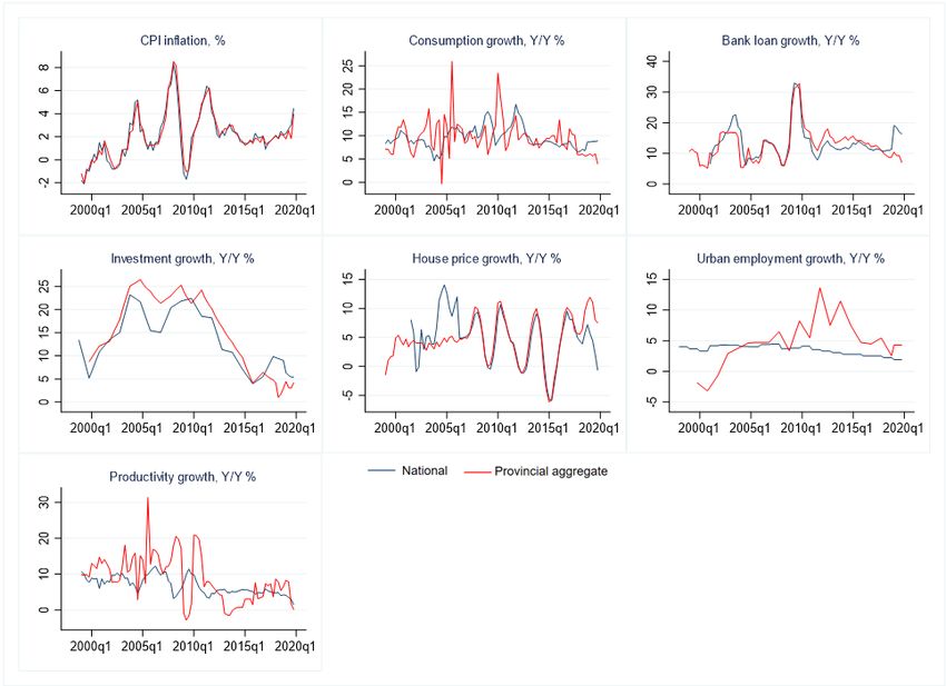
For the other economic variables used in this paper, discrepancies between national and aggregated provincial data
are also rather prominent with consumption, urban employment and productivity. On the other hand, with bank
loan growth, consumer price index, house price growth and investment growth the provincial and national series
seem to match to a high degree. Time series of these economic variables are shown in Figure 9 in Appendix.
3. Data
We use a provincial macroeconomic dataset in quarterly frequency. Table 1 presents all variables and their
summary statistics compared to the corresponding national figures. Series are primarily from the CEIC China
Premium Database that compiles data from different sources. Nominal GDP series, CPI inflation, consumption
expenditures, investments and population come from the National Bureau of Statistics. Bank loan series are
compiled by the People’s Bank of China, regional government expenditures by the Ministry of Finance and urban
employment figures by the Ministry of Human Resources and Social Security. House price data comes from a
Chinese private real estate website owner SouFun-CREIS. Real GDP series is computed by deflating nominal
GDP by CPI inflation. Productivity is computed using real GDP growth and urban employment growth.
Population, urban employment, regional government expenditures and investments are available only at annual
frequency. For population and urban employment, annual values are used for all respective quarters. For
investments and government expenditures, quarterly observations are obtained by linear interpolation. For
consumption and bank loans we have part of the time series in annual frequency (consumption until 2013 and bank
loans until 2003). For 1999-2003 bank loan observations are linearly interpolated to quarterly frequency. Private
consumption observations for 1999-2013 are modified to quarterly frequency using the Denton approach. Table
11 in Appendix gives a more thorough list of the different variables used.
-7-Table 1: Summary statistics, provincial panel and respective national figures
Provincial panel National data
# of obs Mean Std.dev. # of obs Mean Std.dev.
Nominal GDP 2,604 11.37 8.71 88 12.15 4.88
Real GDP 2,604 13.47 9.25 88 8.89 2.19
CPI inflation 2,604 2.10 2.28 82 2.03 2.09
Consumption 2,604 9.62 7.50 79 9.57 2.30
Bank loans 2,604 12.90 8.65 74 13.23 5.37
Investments 2,511 15.65 11.66 81 14.02 5.77
Gov't expenditures 2,511 13.95 9.36 82 16.88 16.22
House prices 2,490 4.61 6.00 71 5.11 4.29
Population 2,387 0.82 1.36 87 0.56 1.00
Urban employment 2,387 4.97 6.71 84 3.57 0.67
Productivity 2,542 9.03 11.38 84 5.45 1.72
Throughout this paper we utilize our provincial data in three different ways. First, we use it as a full panel, all 11
variables for 31 provinces. For the other two ways, we utilize the principal component analysis (PCA), originally
invented by Karl Pearson already in 1901. The idea behind PCA is to ease the interpretation of large datasets by
drastically reducing the number of variables while at the same time retaining as much statistical information as
possible. PCA produces new variables (principal components) that are linear functions of the original dataset and
that are uncorrelated with each other. The first principal component accounts for as much of the variance in the
dataset as possible, and each succeeding component as much of the remaining variance 3. For the second way of
using our provincial data, we compress each of the economic variables across provinces into one component (the
first principal component) at a time, calling these time series the variable specific principal components. For the
third way, we compress the full provincial panel (all economic variables for all provinces) into principal
components. We keep the eight first principal components 4 and call these time series the full information principal
components. In the PCA analysis, all provincial variables are used in year-on-year growth rates and further
standardized to have sample mean zero and unit sample variance.
3
More e.g. in Jolliffe (2002)
4
To determine the number of principal components we could have used e.g. information criteria-type methods (Bai and Ng,
2002). These methods can, however, produce surprisingly divergent conclusions (Hallin, 2007) and are thus far from
conclusive. There also exist older, heuristic methods such as eigenvalue thresholding (Guttman, 1954) and scree plots
(Cattell, 1996) that still are popular methods for factor retention. In our PCA analysis, we keep the eight first principal
components as they all have an eigenvalue above 10 and each can explain at least 4 % of the total sample variance. These
are also the principal components that are in the steep part of the scree plot curve before it flattens out.
-8-Table 2: Proportion of variance explained by principal components
Proportion of variance explained by Proportion of variance explained by first
variable specific principal components eight full information principal components
for each variable in provincial panel for the whole provincial panel
Proportion (%) Proportion (%) Cumulative (%)
Nominal GDP 56.6 % Comp1 22.89 % 22.89 %
Real GDP 50.4 % Comp2 13.16 % 36.05 %
CPI inflation 82.4 % Comp3 9.74 % 45.80 %
Consumption 37.9 % Comp4 6.57 % 52.37 %
Bank loans 57.3 % Comp5 5.63 % 58.00 %
Investments 55.4 % Comp6 5.29 % 63.29 %
Gov't expenditures 35.6 % Comp7 4.21 % 67.50 %
House prices 56.5 % Comp8 3.78 % 71.28 %
Population 39.7 %
Urban employment 52.0 %
Productivity 40.6 %
Looking at the variable specific principal components (first panel, Table 2) for each of the economic variables, we
see that the one for CPI inflation explains the largest amount of variation for the underlying provincial CPI data,
over 82%. Lowest proportion of variance is explained by the variable specific principal components for
government expenditures (35.6%), consumption (37.9%) and population growth (39.7%). The smaller the
proportion that the variable specific principal component can explain, the more prevalent are idiosyncratic shocks
across provinces. On the other hand, larger explanatory power means a stronger underlying common trend.
Turning into the first eight full information principal components obtained by compressing the whole provincial
panel, we see that the first estimated principal component explains 22.9% of the total sample variance, while 13.2%
is explained by the second component. The first eight components explain cumulatively 71% of the total sample
variance. Next, we move on to the empirical estimations.
4. Empirical analysis
This section provides the empirical analysis. First, we show that provincial data is able to explain the majority of
the variation in the national nominal growth rate and further that it is highly informative in projecting national
growth. Using this provincial data, we build an alternative indicator for Chinese growth that is able to reveal
fluctuations not present in the official real GDP growth. Second, we concentrate on the determinants of Chinese
growth and show how the drivers have gone through a substantial change over time both across economic variables
and provinces. We introduce a method to understand the changing nature of Chinese growth that can be updated
regularly using principal components derived from the provincial data.
4.1. Projecting national growth with provincial data
We start by looking how well our provincial panel can project national GDP growth. To this end, we look first at
the proportion of variance the provincial panel can explain of the contemporaneous national GDP, as presented by
Table 3.
-9-Table 3: Proportion of variance in contemporaneous national GDP explained by provincial time series
Variance explained by: National nominal GDP National real GDP
Provincial panel 0.606 0.350
Variable specific principal components 0.878 0.628
Full information principal components 0.893 0.681
When using the whole provincial panel data, we are able to explain 61% of the national nominal GDP’s total
variance. As we compress this panel data into variable specific principal components, the explanatory power
increases to 87.8 %. With the first eight full information principal components, we can explain up to 89.3% of the
variance. What is also imminent from Table 3, is that we are able to explain much less of the variance of the real
GDP.
To find out how well we can project Chinese growth with provincial data, we begin by conducting granger
causality tests. Our dependent variable is the national nominal GDP growth. As explanatory variables, we have
the lagged value of the dependent variable and the lagged values of the provincial variables. We first use the full
provincial panel and in turn replace the explanatory variables by the variable specific principal components and
then by the eight full information principal components. We use the four-quarter lagged values for all explanatory
variables. Table 4 presents the results.
Table 4: Granger causality test results: provincial panel, variable specific and full information principal components
Provincial panel Variable specific principal components Full information principal components
Overa l l R2 0.606, # obs : 2400 Overa l l R2 0.814, # obs : 80 Largest factor loadings in parentheses Overa l l R2 0.821, # obs : 80
Marginal Marginal Marginal
Coeff F-stat Prob>F R2 Coeff F-stat Prob>F R2 Coeff F-stat Prob>F R2
Inflation -1.469 929.49 0.000 0.201 pc(inflation) -0.961 51.65 0.000 0.154 Pc 3 (Credit + inv. - infl. - house prices) 0.486 57.64 0.000 0.249
Credit 0.128 164.53 0.000 0.030 pc(credit) 0.277 18.22 0.000 0.024 Pc 6 (House prices + inv. - consumption) 0.437 47.77 0.000 0.077
Investments 0.078 109.23 0.000 0.018 pc(investments) 0.368 8.89 0.004 0.014 Pc 2 (Productivity - urban empl.) 0.197 38.40 0.000 0.094
Productivity 0.040 23.99 0.000 0.003 pc(consumption) -0.325 6.83 0.011 0.010 Pc 8 (Consumption - gov't expend.) 0.237 10.47 0.002 0.028
House prices -0.051 12.21 0.001 0.013 pc(productivity) 0.438 6.61 0.012 0.011 Pc 4 (House prices - gov't expend.) 0.170 6.78 0.009 0.015
Consumption -0.032 10.92 0.001 0.002 pc(gov't exp.) -0.168 1.77 0.187 0.002 Pc 7 (Productivity + consumption) -0.004 5.64 0.020 0.013
Gov't expend. -0.011 1.35 0.245 0.000 pc(population) -0.140 1.59 0.212 0.003 Pc 5 (House prices + credit) -0.030 0.08 0.776 0.000
Population -0.054 0.91 0.341 0.000 pc(urban empl.) 0.208 1.45 0.233 0.003 Pc 1 (GDP + investments) -0.001 0.08 0.777 0.000
Urban empl. 0.008 0.35 0.553 0.000 pc(house prices) -0.114 0.88 0.351 0.005
Notes: Dependent variable nominal national GDP growth. All explanatory variables lagged by 4 quarters and sorted by their Prob>F-stat. Lagged dependent variable omitted from table.
The left most part of the table presents the granger causality results for the provincial panel variables. The first six
provincial variables are statistically significant in explaining future national growth at the 1% level. These are
inflation, credit, investments, productivity, house prices and consumption. The lagged provincial variables can
explain a total of 61% of the total variance of future national growth.
Using the full provincial panel, we are forcing the coefficients for each variable to be the same across provinces.
The rest of the table looks at whether the results hold in time series, i.e. after compressing the provincial panel into
principal components. Using the variable specific principal components (middle section of the table) and full
information principal components (right part of the table) we allow different factor loadings for each province and
each variable.
- 10 -We find that the result holds in time series, so that also the compressed components are highly significant in
projecting Chinese aggregate growth 5. The first three variable specific principal components are statistically
significant in projecting future national growth at the 1 % level. These are inflation, credit and investments. With
full information principal components, there are five components that are statistically significant in explaining
future aggregate growth at the 1 % level and these are components number three, six, two, eight and four (sorted
by their probabilities in explaining future national growth) 6. With lagged variable specific and full information
principal components we can explain 81 % and 82 % of the total variance of aggregate national growth,
respectively.
In all, the provincial data seems to be highly relevant and provides information able to explain the majority of the
variance of national growth. For that reason, the provincial data is an excellent candidate when thinking about
alternative indicators for Chinese growth. As discussed in the introduction, there exists a long-standing debate
over the reliability of China’s GDP figures and especially after the real GDP growth series became flat since 2012,
several alternative growth measures have emerged. We contribute to the search of missing fluctuations by
computing three candidates as alternative growth indicators using the provincial data. For the first alternative
growth indicator, we regress the national nominal GDP growth on its own lagged value and the lagged values of
the full information principal components that were statistically significant in the granger causality tests presented
in Table 4 (full information principal components 3, 6, 2, 8 and 4). For the second alternative growth indicator,
we replace as explanatory variables the statistically significant variable specific principal components. These are
the variable specific principal components of inflation, credit and investments. For the third alternative growth
indicator, we use as explanatory variables the unaltered provincial variables that were statistically significant in
Table 4: inflation, credit, investments, productivity, house prices and consumption. To assess the relative accuracy
of these candidates, we compute cross-correlations between official growth rates and different alternative growth
indicators.
Table 5 presents the cross-correlation of the official national growth rates (nominal and real), the Li Keqiang index,
two publicly available Business Cycle Indicators (one by the NBS and one by the PBoC), as well as our three
different growth indicator candidates constructed from the provincial panel.
5
Instead of using static principal component analysis in economic forecasting à la Stock and Watson (2002) another option
would be to use dynamic principal component analysis as in Forni et al. (2000). However, as it very likely would not
increase the performance of our analysis (e.g. D’Agostino and Giannone, 2006; Boivin and Ng, 2005) but rather make the
economic interpretation more difficult, we stick to the static principal component analysis.
6
The first principal component is statistically insignificant and only able to explain less than 0.0 % of the total variance.
Reason is that it was compressed initially from the full provincial panel where it explained 22.9 % of the total sample
variance. Here we force the principal components to explain only one time series, namely the future national nominal GDP
growth.
- 11 -Table 5: Cross-correlation between official growth rates and alternative growth indicators, contemporaneous values
Alternative growth indicators
(1) (2) (3)
Business Business Using Using Using
National National Li Climate Climate stat.sign. stat.sign. stat.sign.
nominal real Keqiang Index, Index, full info var spec. provincial
GDP GDP index NBS PBoC PCs PCs vars
National nominal GDP 1.00
National real GDP 0.84 1.00
Li Keqiang index 0.56 0.75 1.00
Business Climate Index, NBS 0.84 0.68 0.49 1.00
Business Climate Index, PBoC 0.87 0.82 0.65 0.83 1.00
Alternative 1) Using statistically significant full information principal components* 0.90 0.78 0.50 0.78 0.88 1.00
growth 2) Using statistically significant variable specific principal components** 0.89 0.82 0.47 0.79 0.89 0.95 1.00
indicators
3) Using statistically significant provincial variables*** 0.73 0.65 0.37 0.66 0.79 0.81 0.85 1.00
* Full information principal components PC2, PC3, PC4 PC6 and PC8. ** Variable specific principal components: pc(inflation), pc(credit) and pc(investments) *** Provincial variables: inflation,
credit, investments, productivity, house prices and consumption
All alternative indicators computed by regressing nominal aggregate growth on its own (4 quarter) lagged value and the (4 quarter) lagged values of the statistically significant variables.
When using the unaltered provincial panel variables (the third alternative growth indicator), we have a correlation
of 0.73 with the national nominal GDP and 0.65 with the real GDP. However, for the second and first alternative
growth indicators, we have much higher correlation coefficients. Using variable specific principal components,
the correlation is 0.89 with nominal and 0.82 with real GDP growth. With statistically significant full information
principal components, the correlation is 0.90 with nominal and 0.78 with real GDP growth. The second and first
alternative indicators are also highly correlated with the Business Climate Indices (correlation 0.78–0.89). We
ultimately choose the first alternative as our main growth indicator, as it uses full information principal components
and thus a larger amount of information from the panel than the second alternative. We name it 31 Provinces China
Business Cycle Indicator (31P-CBCI). Figure 3 presents the 31P-CBCI alongside with official national GDP
growth rates 7.
Figure 3: 31 Provinces China Business Cycle Indicator
31 Provinces - China Business Cycle Indicator
25
25
20
20
Fitted values
Y/Y, %
15
15
10
10
5
5
1998q1 2000q1 2002q1 2004q1 2006q1 2008q1 2010q1 2012q1 2014q1 2016q1 2018q1 2020q1
31P-CBCI
National nominal GDP growth
National real GDP growth
7
First and second alternative indicators are broadly similar in shape throughout the last two decades. Figure 10 in Appendix
provides a similar presentation of the second alternative indicator.
- 12 -As we use nominal GDP series when fitting the 31P-CBCI, its level is by construction closer to the level of the
nominal than to the real growth rate. However, we are more interested to uncover business cycle fluctuations,
which the official real GDP flattens out, than the actual level of the growth rate. Given our endeavor to extract
these fluctuations and not growth rate levels, we standardize the three series to have zero mean and unit standard
deviation (Figure 4) 8.
Figure 4: 31P-CBCI and official GDP growth rates, standardized series with zero mean and unit standard deviation
31P-CBCI and official GDP growth rates, standardized
2
1.5 1
Std. deviation
-.5 0 -1.5
-1.5
-2
2000q1 2002q1 2004q1 2006q1 2008q1 2010q1 2012q1 2014q1 2016q1 2018q1 2020q1
31P-CBCI Real GDP growth Nominal GDP growth
Based on the 31P-CBCI, there was an increase in growth rate in 2015, followed by a drop in 2016. We observe an
abrupt acceleration of growth in 2017 and a loss of steam starting at the beginning of 2018 and further weakening
during 2019. This contrasts with the steadiness of official growth series. In nominal terms, GDP growth decelerated
between 2014 and 2015, then increased fast during the second half of 2016 and started to fall again after 2017. In
real terms, growth rate is rather constant but what both official series indicate is that growth in 2019 Q4 was around
one standard deviation below its trend. The 31P-CBCI points to a much lower growth rate relative to its trend at
the end of the time span.
To further illustrate how each full information principal component contributes to the formation of the 31P-CBCI
over time, we illustrate in Figure 5 the contributions of all the dependent variables (lagged nominal GDP growth
and lagged full information principal components 2,3,4,6 and 8). In the figure, series’ labels present the largest
factor loadings for each principal component to better assess which macroeconomic variables are the main drivers.
Factor loadings are more thoroughly discussed later in section 4.2.
8
Data for standardized 31P-CBCI will be updated quarterly as new provincial data becomes available and published at the
Bank of Finland BOFIT webpage. Data is downloadable. https://www.bofit.fi/en/monitoring/statistics/china-statistics/
- 13 -Figure 5: Contribution of variables behind 31P-CBCI over time
Principal component 2 (reflecting developments in productivity and urban employment) contributes to Chinese
growth mostly positively in the first half of the sample and mostly negatively in the second half of the sample,
notably in the aftermath of the great financial crisis. Principal component 3 (strongest drivers being credit and
investment relative to inflation and house prices) contributes to growth fluctuations with a strong cyclical pattern.
It alternates periods where it pushes growth up and down for up to 3 years for each phase. Up-phases include 2003-
2004, 2010-2012, 2015-2016 and down-phases 2001-2002, 2008-2009 and 2017-2019. In more recent years, it
seems to be the main contributor to both the upturn of 2015 as well as the largest downward pulling factor for
years 2018 and 2019. While the upturn of 2015 was mostly driven by principal component 3, the more recent
acceleration of growth in 2017 had other drivers. There, we observe a combination of contributions from principal
component 8 (consumption and government expenditure), principal component 6 (house prices, investments and
consumption) and principal component 4 (house prices and government expenditure).
This figure also reveals that the contribution of the lagged dependent variable (nominal GDP growth) is quite
large. However, we show in Appendix that excluding this lagged nominal GDP does not change our results. Figure
11 in Appendix presents an optional growth indicator computed using only our eight full information principal
components, discarding the lagged nominal GDP growth. As can be seen, differences between this optional
indicator and the 31P-CBCI are minimal and we thus stick to our more parsimonious model. Figure 12 in Appendix
breaks this optional indicator into its driving principal components the same way as Figure 5 for the 31P-CBCI.
What stands out in Figure 12 is that it sharpens our take on the most recent upturn in 2017 confirming it to be
mostly demand driven, as principal component 7 (reflecting developments in productivity and consumption) seems
to have the strongest positive contribution. Moreover, principal component 7 also appears as a negative contributor
to growth in 2019. This points to the conclusion that the growth decline that started in 2018 broadened to the
demand side during 2019.
Next, we look more closely to the determinants of the Chinese growth and how they have changed during the past
two decades.
- 14 -4.2. Determinants of Chinese growth
We begin by taking a closer look at the five full information principal components that were found to be statistically
significant in explaining future aggregate growth (Table 4, section 3.1.) and were used in building the 31P-CBCI.
The principal components are estimated using the whole provincial panel, so they compress information from all
the economic variables for 31 provinces. Figure 6 presents the time series of these five principal components and
Table 6 their factor loadings.
Table 6: Factor loadings of the full information principal components
Factor Factor Factor Factor Factor
Principal component 2 loading Principal component 3 loading Principal component 4 loading Principal component 6 loading Principal component 8 loading
Productivity 1.318 Credit 3.197 house prices 2.093 house prices 1.578 consumption 1.036
Population 0.756 Investments 1.488 consumption 1.408 Investments 1.256 Real GDP 0.408
Gov't expenditures 0.646 consumption 1.045 Real GDP 1.187 Credit 0.729 Urban employment 0.288
Real GDP 0.465 Real GDP 0.820 Nominal GDP 0.764 Gov't expenditures -0.121 Nominal GDP 0.281
consumption 0.383 Urban employment 0.562 Productivity 0.490 Productivity -0.252 Population 0.195
house prices -0.173 Nominal GDP 0.159 Urban employment 0.439 Population -0.317 Productivity 0.169
Nominal GDP -0.194 Gov't expenditures 0.013 Credit 0.257 Real GDP -0.327 Credit 0.063
Investments -0.257 Population -0.141 Population -0.694 Nominal GDP -0.506 house prices -0.016
Credit -0.985 Productivity -0.341 Investments -1.305 Urban employment -0.625 Inflation -0.326
Inflation -2.455 house prices -1.812 Inflation -1.339 Inflation -0.660 Investments -0.349
Urban employment -2.567 Inflation -2.164 Gov't expenditures -1.694 consumption -1.372 Gov't expenditures -0.761
Principal component 2 has highest factor loadings in productivity and urban employment, the latter with a minus
sign. Hence, we consider this principal component to give an indication on the fluctuation of “productivity in urban
areas”. Principal component 3 has highest positive factor loadings in credit and investments and highest negative
factor loadings in inflation and house prices, it is therefore an indicator of “credit in real terms”. Principal
component 4 has highest factor loadings in house prices and government expenditures, the latter with a minus sign,
a combination of variables that is more difficult an interpretation. Principal component 6 has highest positive factor
loadings in house prices and investments and highest negative with consumption. It can be seen as indicating the
deviations of investment from consumption. Finally, principal component 8 has highest positive factor loading in
consumption and highest negative in government expenditures, it captures the difference between private
consumption and government expenditures.
- 15 -Figure 6: Five full information principal components statistically significant in explaining future aggregate growth
20
10
Y/Y, %
0
-10
-20
1998q1 2000q1 2002q1 2004q1 2006q1 2008q1 2010q1 2012q1 2014q1 2016q1 2018q1 2020q1
Pc 2 Pc 3 Pc 4 Pc 6 Pc 8
Nominal GDP growth
Note: dashed line for Pc 4 denotes correlation turning negative after 2010 in Table 7
To further assess the combination of macroeconomic variables pulling aggregate growth, we regress the national
GDP growth on these five full information principal components. All explanatory variables, including the lagged
dependent variable, are lagged by four quarters. Results are presented in Table 7 (left panel) where principal
components used as explanatory variables are sorted by their marginal R-squared values for the entire sample.
Table 7: Regression results, dependent variable national nominal GDP growth
Principal components with largest factor loadings Whole time span Before 2010 After 2010
Ma rgi na l Ma rgi na l Ma rgi na l
Coeff. t P >|t| R2 Coeff. t P >|t| R2 Coeff. t P >|t| R2
National GDP growth (lagged) 0.561 9.19 0.000 0.275 0.799 3.8 0.001 0.086 0.568 6.73 0.000 0.234
Pc3: Credit + investments - inflation - house prices 0.485 10.90 0.000 0.322 0.699 4.87 0.000 0.122 0.319 5.70 0.000 0.107
Pc6: House prices + investments - consumption 0.438 9.43 0.000 0.142 0.557 4.31 0.000 0.076 0.513 4.19 0.000 0.077
Pc2: Urban employment - productivity 0.196 6.20 0.000 0.072 0.366 2.08 0.047 0.024 0.262 2.07 0.046 0.015
Pc8: Consumption - gov't expenditures 0.238 7.17 0.000 0.030 0.222 1.70 0.100 0.015 0.348 3.04 0.005 0.026
Pc4: House prices - gov't expenditures 0.169 4.34 0.000 0.026 0.124 1.14 0.263 0.005 -0.119 -1.20 0.237 0.004
Number of obs erva ti ons 77 37 40
R-squared 0.834 0.810 0.879
Note: Dependent variable: nominal aggregate GDP growth. All four quarter lagged values.
Looking first at the full sample, we find that Chinese aggregate growth is driven predominantly by credit and
investments (over inflation and house prices), i.e. credit and investment in real terms. Principal component 3
clearly has the highest marginal R-squared explaining for around 32 % of the total variance of future aggregate
growth. Principal component 6, which captures the difference between house prices and investments with respect
to consumption, explains around 14 % of the total variance of Chinese nominal growth rate. Principal component
- 16 -2 explains around 7 % of the total variance and reflects developments in the productivity of urban employment.
Thus, what our statistical model of Chinese growth suggests is that national growth for the last two decades has
been mainly grounded on credit, investments and house prices as well productivity of its urban areas.
Next, we want to assess whether these drivers of Chinese growth have evolved over time. Throughout the first
decade of the 21st century, China grew at an accelerating pace reaching 15 % year-on-year just before the financial
crisis. Growth was primarily based on resource-intensive manufacturing, exports and low-paid labor. Since then,
growth has moderated. Several structural constraints, such as decreasing workforce, slowing productivity, limits
to internal migration and ongoing shift towards a more service-based economy are likely causal factors of this
deceleration. Furthermore, the financial crisis outlined the vulnerabilities of an export-led growth strategy. As a
result, China started to put more emphasis on domestic demand, self-sufficiency and economic independence.
We divide our sample period in two equally sized sub-periods, before and after 2010. This way we can consider
the decade before the great financial crisis separately from the years of more moderate growth. The second sub-
period is also the one during which China officially aimed to double its real GDP and became more or less fixated
with numerical growth targets.
To examine how the growth drivers have changed, we explore our provincial data further in three different ways.
As a simple first experiment, we redo the previous regression separately for these two sub-periods, before and
after 2010. Results are presented in Table 7 center and right panels. Principal components used as explanatory
variables are the same for both sub-samples and for the full time span. When looking at the reported regression
coefficients, it is immediately evident that most of the growth determinants have a higher marginal R-square for
the entire sample than for each of the sub-samples. This means that the full information principal components that
we estimate over the full sample capture persistent phenomena and changes in fluctuations that are relevant across
the two sub-samples.
We also find that several of the principal components are relevant in either samples. Their marginal R-square,
although smaller than for the full sample for some, have been remarkably stable. The main exception is PC4 that
reflects differences between government and private sector expenditures, which changes sign. Strikingly, we
observe that this faster public expenditure pull growth down before 2010 and up thereafter. We also see a decline
in the estimated coefficients for principal components 2 that reflects urban productivity and 3 that reflects real
credit and investment. These changes would suggest that real credit and investment and urban employment and
productivity matter somewhat less to aggregate growth after 2010.
4.3. Determinants of Chinese growth: further insights from the 31 Chinese provinces
We dive one step further into the province level data to gain further insights on Chinese growth. We assess whether
what is true for the aggregate also applies to individual Chinese provinces. As discussed in the introduction, there
exists significant heterogeneity across provinces in terms of growth, cycles and structural changes. Exploiting the
dataset for 31 provinces, we can study how each province fits into the empirical model of Chinese growth presented
in Table 7.
Our approach is to construct for each province its representation in our full information factor model shown in
table 7. This representation is obtained by building full information principal components 2, 3, 4, 6 and 8 for each
province using the factor loadings for each economic variable as in Table 6 and the respective economic variable
time series for each province. We then multiply the obtained regional principal components 2, 3, 4, 6 and 8 by
model coefficients presented in Table 7 (left most panel). As a result, we have 31 time series representing our full
information factor model for each province. In order to see how well these provincial models are correlated with
- 17 -future aggregate growth, we compute the correlation coefficients between provincial models and aggregate
national growth. Correlation coefficients for each province are presented in Table 12 in the Appendix.
Figure 7 helps to visualize these results. For a majority of provinces, our statistical model of Chinese growth
applied to economic developments in the province is positively correlated with national growth in China, This is
the case of all (light and dark) blue provinces. This is not the case however for pink provinces (four provinces in
the far west, Xinjiang, Tibet, Qinghai and Gansu, Heilongjiang in the far north-east as well as two provinces –
Hubei and Guizhou – in central China). For these, our statistical model of Chinese growth does not apply, i.e.
growth in these provinces has had other determinants than the ones that prevail at the national level and for a
majority of provinces.
Provinces with statistically significant correlation with future national aggregate growth are further divided in two
depending on whether the correlation is above or below the median of the statistically significant correlation
coefficients. If correlation is above (below) median, province is colored in dark (light) blue. Provinces with the
strongest statistically significant correlation (dark blues) are scattered mostly in the coastal region.
Figure 7: Correlation between provincial growth model and future aggregate growth, full time span
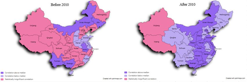
We now turn to the evolution of the determinants of growth before and after 2010 by computing the correlation of
the province level model prediction with national nominal growth for each sub-sample. The shift across provinces
is presented by the two maps in Figure 8. Again, blue represents provinces that are correlated with future aggregate
growth and pink represents statistically insignificant correlation. The model applies to a much larger number of
provinces since 2010, as growth has become more homogeneous across provinces. Only Xinjiang and Tibet
(Xizang) remain uncorrelated with national growth for both subsamples.
- 18 -Figure 8: Correlation between provincial growth model and future aggregate growth, two different time spans
As a second way to study changes in the determinants of growth, we continue to dig a bit deeper into the analysis
of provincial data. We use the grouping of provinces presented in Figure 7 to compare the determinants of growth
with panel regressions across blue and pink provinces 9, both for the full sample and for each sub samples.
Importantly, we include the national growth rate as a control variable to capture province specific developments.
Table 8 presents these panel regression results 10.
9
Doing the groupings based on correlations with the province level GDP growth obtains very similar groupings and hence
regression results.
10
We note that both the lagged provincial inflation and lagged national GDP are highly significant in all specifications.
Further, the coefficient of provincial inflation is negative, which may seem somewhat puzzling at first. However, as
inflation is by default included in the nominal GDP series, this negative coefficient is likely to be some form of mean
reversion correcting for the coefficient of the lagged nominal GDP. Indeed, if excluding the lagged dependent variable, the
coefficients of provincial inflation lose some or all their statistical significance and even become positive in some of the
specifications.
- 19 -You can also read