People Meet People - A Microlevel Approach to Predicting the Effect of Policies on the Spread of COVID-19
←
→
Page content transcription
If your browser does not render page correctly, please read the page content below
Discussion Paper Series – CRC TR 224

                                       Discussion Paper No. 265
                                           Project A 02, C 01

         People Meet People - A Microlevel Approach to
    Predicting the Effect of Policies on the Spread of COVID-19

                                              Janos Gabler 1
                                              Tobias Raabe 2
                                               Klara Röhrl 3

                                              February 2021

       1
           Bonn Graduate School of Economics (University of Bonn) and IZA Institute of Labor Economics
                                                2
                                                  Unaffiliated
                          3
                            Bonn Graduate School of Economics (University of Bonn)

Funding by the Deutsche Forschungsgemeinschaft (DFG, German Research Foundation)
                  through CRC TR 224 is gratefully acknowledged.

                     Collaborative Research Center Transregio 224 - www.crctr224.de
                  Rheinische Friedrich-Wilhelms-Universität Bonn - Universität Mannheim
People Meet People - A Microlevel Approach to
Predicting the Effect of Policies on the Spread of
Covid-19 ?
Janoś Gabler a, b
Tobias Raabe c
Klara Röhrl a
a
Bonn Graduate School of Economics
b
IZA Institute of Labor Economics
c
Unaffiliated
December 2020
This version: February 9, 2021
Governments worldwide have been adopting diverse and nuanced policy measures to
contain the spread of Covid-19. However, epidemiological models usually lack the de-
tailed representation of human meeting patterns to credibly predict the effects such
policies. We propose a novel simulation-based model to address these shortcomings.
We build on state-of-the-art agent-based simulation models, greatly increasing the
amount of detail and realism with which contacts take place. Firstly, we allow for
different contact types (such as work, school, households or leisure), distinguish re-
current and non-recurrent contacts and allow the infectiousness of meetings to vary
between contact types. Secondly, we allow agents to seek tests and react to informa-
tion, such as experiencing symptoms, receiving a positive test or a known case among
their contacts, by reducing their own contacts. This allows us to model the effects of
a wide array very targeted policies such as split classes, mandatory work from home
schemes or test-and-trace policies. To validate our model, we show that it can pre-
dict the effect of the German November lockdown even if no similar policy has been
observed during the time period that was used to estimate the model parameters.
JEL Classification: C63, I18
Keywords: Covid-19, agent based simulation model, public health measures
?
Gabler and Röhrl are grateful for financial support by the German Research Foundation (DFG)
through CRC-TR 224 (Projects C01 and A02, respectively). Gabler is grateful for funding by IZA Insti-
tute of Labor Economics. We gratefully acknowledge support from the Google Cloud COVID-19 research
credits program.
11 Introduction
The first wave of the Covid-19 pandemic prompted strict lockdowns and restrictions
across the world. At large social and economic costs, these strict measures were able
to suppress the spread of the disease in many countries and allowed governments to
relax restrictions over the summer. When infections started to soar again in the fall,
governments were more hesitant and imposed less restrictive policies. For example,
Germany imposed a “lockdown-light” in November, closing fewer businesses than in
spring and leaving schools open.
The less restrictive lockdowns proved insufficient to stop the second wave, lead-
ing many experts to call for a strict lockdown to bring cases back to very low lev-
els, such as single digit incidences (for example Priesemann, Brinkmann, Ciesek,
Cuschieri, Czypionka, et al. (2021)). These calls have received additional attention
since new and more contagiuos variants have emerged in across the globe (Duong,
2021) and increased the urgency to reduce transmission dynamics and increased
awareness for the mutagenic threat posed by high incidences. Given the importance
to bring down and maintain low infection numbers until vaccinations reach herd
immunity levels, it is paramount for policy makers and the public to understand the
effectiveness and trade-offs involved in different policies.
However, epidemiological models are not suited for this task. As they have not
been designed to predict the effects of fine-grained policies, they need to be ex-
tended for each new policy proposal.
This report describes a model that has been designed from the ground up to
predict the effects of contact reducing policies in real time. It has the following
features:
(1) At the core of the model, people meet people based on a matching algorithm. We
distinguish various types of contacts. The contact types are households, leisure
activities, schools, preschools, and nurseries and several types of contacts at the
workplace. Contact types can be random or recurrent and vary in frequency.
(2) Policies can be implemented as shutting down contact types entirely or partially.
The reduction of contacts can be random or systematic. For example, it is possi-
ble to implement split class schooling where only one half of each class attends
and the attending half switches on a weekly bases.
(3) Infection probabilities vary across contact types and reflect properties of the
contact like the location (indoor/outdoor) and the kind of interaction (dura-
tion, physical contact). The probabilities are independent from the number of
contacts and, thus, policy-invariant.
(4) The model achieves a good fit on German data of infection rates even if only
the infection probabilities are fit to the data and the remaining parameters are
calibrated from the medical literature and datasets on contact frequencies and
mobility reductions.
1(5) High quality Python code for the model is freely available on Github, well docu-
mented and very flexible1. We are actively looking for researchers who want to
use our model for their projects and apply it to other contexts.
This report describes the model in an abstract way, but uses many realistic ex-
amples from a version that is specialized to Germany. It is important to note that
it would be easy to adjust the model to other countries if data on the number of
contacts and a dataset with background characteristics are available.
More details about the German model as well as applications to currently dis-
cussed German policies can be found in Dorn, Gabler, Gaudecker, Peichl, Raabe,
et al. (2020), Gabler, Raabe, Röhrl, and Gaudecker (2020), and Gabler, Raabe,
Röhrl, and Gaudecker (2021).
The report proceeds as follows: In Section 2, we give a short overview of epidemi-
ological models. We continue with a detailed description of our model in Section 3
and proceed with a description of model parameters and the estimation in Section 4.
The model is validated in Section 5 by assessing the in-sample fit for reported infec-
tions from August to October and by comparing the out-of-sample fit for the period
from November until the beginning of Christmas for different lockdown scenarios.
We conclude in Section 6.
2 Literature Review
We build on two strands of literature: Recent extensions of the epidemiological SEIR
model and agent-based simulation models.
The traditional SEIR model is not fine-grained enough to model nuanced poli-
cies. This has motivated a large number of researchers to extend the standard model
to allow for more heterogeneity and flexibility. Examples are Grimm, Mengel, and
Schmidt (2020), Donsimoni, Glawion, Plachter, and Wälde (2020) and Acemoglu,
Chernozhukov, Werning, and Whinston (2020) who develop multi group SEIR mod-
els to analyze the effects of targeted lockdowns and Berger, Herkenhoff, and Mon-
gey (2020) who extend the SEIR model to analyze testing and conditional quaran-
tines. For a more comprehensive review see Avery, Bossert, Clark, Ellison, and Ellison
(2020). Others have used the results of a standard SEIR model as input for economic
models that estimate the cost of policies (e.g. Dorn, Khailaie, Stöckli, Binder, Lange,
et al. (2020)).
While the popularity of the SEIR model is mainly due to its simplicity, the exten-
sions are quite complex. It is unlikely that there will be a SEIR model that combines
all proposed extensions. Moreover, the extensions do not address other key issues:
1. The code can be found under https://github.com/covid-19-impact-lab/sid and the documenta-
tion with tutorials and background information under https://sid-dev.readthedocs.io/.
2The main parameter of the SEIR model, the basic reproduction number (R0 ), is not
policy-invariant. It is a composite of the number of contacts each person has and the
infection probability of the contacts. In fact, policy simulations are done by setting
R0 to a different value but it is hard to translate a real policy into the value of R0 it
will induce. In other words, SEIR models are not suited for evaluating the effect of
policies which have never been experienced before.
Another commonly used model class in epidemiology are agent-based simula-
tion models. In these models individuals are simulated as moving particles. Infec-
tions take place when two particles come closer than a certain contact radius (e.g.
Silva, Batista, Lima, Alves, Guimarães, et al. (2020) and Cuevas (2020)). While the
simulation approach makes it easy to incorporate heterogeneity in disease progres-
sion, it is hard to incorporate heterogeneity in meeting patterns. Moreover, policies
are modeled as changes in the contact radius or momentum equation of the parti-
cles. The translation from real policies to corresponding model parameters is a hard
task.
Hinch, Probert, Nurtay, Kendall, Wymatt, et al. (2020) is a recent extension
of the prototypical agent-based simulation model that replaces moving particles by
contact networks for households, work and random contacts. This model is similar
in spirit to ours but focuses on contact tracing rather than social distancing policies.
The above assessment of epidemiological models is not meant as a critique. We
are aware that these models were not designed to predict the effect of fine-grained
social distancing policies in real time and are very well suited to their purpose. We
invite epidemiologists to provide feedback and collaborate to improve our model.
3 Model
3.1 Summary
To predict the effects of a wide variety of fine-grained social distancing policies
we propose a different model structure. Our model inherits many features from
agent-based simulation models but replaces the contacts between moving particles
by contacts between individuals who work, go to school, live in a household and
enjoy leisure activities. The structure of the model is depicted in Figure 1.
The background characteristics include age, county and occupation of each sim-
ulated individual. Contact models are functions that map individual characteristics
into a predicted number of contacts. Currently, we distinguish between eight types
of contact models which are all listed in Figure 1: households, recurrent and ran-
dom work contacts, recurrent and random leisure contacts, and nursery, preschool,
and school contacts.
The predicted number of contacts is translated into infections by a matching al-
gorithm. There are different matching algorithms for recurrent contacts (e.g. class-
3Figure 1. Simplified graph of the model.
mates, family members) and non-recurrent contacts (e.g. clients, contacts in super-
markets). The infection probability can differ for each contact type. All types of
contacts can be assortative with respect to geographic and demographic character-
istics.
Once a person is infected, the disease progresses in a fairly standard way which
is depicted in Figure 2. Asymptomatic cases and cases with mild symptoms are infec-
tious for some time and recover eventually. Cases with severe symptoms additionally
require hospitalization and lead to either recovery or death.
Our model also allows the evaluation of different testing strategies by having
a detailed three-step model of test demand, allocation and processing: First, indi-
viduals demand a test because they, e.g., experience symptoms. Secondly, tests are
allocated to individuals while respecting governmental access restrictions to tests.
Thirdly, depending of the capacities of laboratories, tests are processed for some
time until the individual receives her test result. This framework would allow to
evaluate the effect of different testing demand behavior and allocation policies, as
are for example discussed by Tröger et al. (2020).
In addition, people who have symptoms, received a positive test, or had a risk
contact can reduce their number of contacts across all contact types endogenously.
The model makes it very simple to translate policies into model quantities. For
example, school closures imply the complete suspension of school contacts. A strict
lockdown implies shutting down work contacts of all people who are not employed
in a systemically relevant sector. It is also possible to have more sophisticated policies
that condition the number of contacts on observable characteristics, risk contacts or
health states.
Another key advantage of the model is that the number of contacts an individual
has of each contact type can be calibrated from publicly available data (Mossong,
4Hens, Jit, Beutels, Auranen, et al., 2008). This in turn allows us to estimate policy-
invariant infection probabilities from time series of infection and death rates using
the method of simulated moments (McFadden, 1989). Since the infection probabil-
ities are time-invariant, data collected since the beginning of the pandemic can be
used for estimation. Moreover, since we model the testing strategies that were in
place at each point in time, we can correct the estimates for the fact that not all
infections are observed.
Last but not least, performing simulations whose starting point is set amidst the
pandemic requires special adjustments to arrive at a realistic distribution of courses
of diseases. We solve the initial conditions problem by matching reported infections
to individuals in our data while also correcting for reporting lag and undetected
cases.
In the following sections we describe each of the model components in more
detail.
3.2 Modeling Numbers of Contacts
Consider a hypothetical population of 1,000 individuals in which 50 were infected
with a novel infectious disease. From this alone, it is impossible to say whether only
those 50 people had contact with an infectious person and the disease has an infec-
tion probability of 1 in each contact or whether everyone met an infectious person
but the disease has an infection probability of only 5 percent per contact. SEIR mod-
els do not distinguish contact frequency from the infectiousness of each contact and
combine the two in one parameter that is not invariant to social distancing policies.
To model social distancing policies, we need to disentangle the effects of the
number of contacts of each individual and the effect of policy-invariant infection
probabilities specific to each contact type. Since not all contacts are equally infec-
tious, we distinguish different contact types.
The number and type of contacts in our model can be easily extended. Each type
of contacts is described by a function that maps individual characteristics, health
states and the date into a number of planned contacts for each individual. This
allows to model a wide range of contact types.
Currently, there are the following contact types:
• Households: Each household member meets all other household members every
day. The household sizes and structures are calibrated to be representative for
Germany.
• Random non-work contacts: Each person has contacts with randomly drawn
other people which are assortative with respect to region and age group. This
contact type reflects contacts during pure leisure activities as well as non leisure
activities such as grocery shopping or medical appointments.
5• Recurrent daily non-work contacts: Each person has daily recurring contacts
which allows to model close relationships other than families between individu-
als.
• Recurrent weekly non-work contacts: Each person has weekly recurring contacts
like sports groups or other weekly activities.
• Random work contacts: Each working adult has contact to randomly drawn
other people at work.
• Recurrent daily work contacts: Each working adult meets other workers every
day. This is meant to capture work colleagues.
• Recurrent weekly work contacts: Each working adult meets other workers once
per week. We randomize over the days on which the meetings take place. This
is meant to capture meetings with clients, superiors or other colleagues which
happen infrequently.
• Schools: Each student meets all of his classmates every day. Class sizes are
calibrated to be representative for Germany and students have the same age.
Schools are closed on weekends and during vacations, which vary by states.
School classes also meet three pairs of teachers every school day. The pairs are
meant to represent interactions between teachers.
• Preschools: Children who are at least three years old and younger than six may
attend preschool. Each group of nine children interacts with the same two adults
every day. The children in each group are of the same age. The remaining me-
chanics are similar to schools.
• Nurseries: Children younger than three years may attend a nursery and interact
with one adult. The age of the children varies within groups. The remaining
mechanics are similar to schools.
The number of random and recurrent contacts at the workplace, during leisure
activities and at home is calibrated with data provided by Mossong et al. (2008).
For details see Section 3.2. In particular, we sample the number of contacts or group
sizes from empirical distributions that sometimes depend on age. It is also possible
to use economic or other behavioral models to predict the number of contacts.
Theoretically, each contact type can have its own infection probability. However,
to reduce the number of free parameters and thus avoid a potential over-fitting
we impose some constraints. For now, infection probabilities in schools, preschools
and nurseries are equal. Moreover, we restrict all work contacts and all non-work
contacts to have the same infection probability.
3.3 Reducing Numbers of Contacts Through Policies
The main motivation of our model is to predict the effect of policies that affect the
number of contacts people have. Examples range from school closures and lock-
downs to more nuanced policies such as mandatory quarantines for symptomatic
6individuals or a class splitting policy where only half of the students come to school
in person and the other half joins digitally with weekly rotation.
Instead of thinking of policies as completely replacing how many contacts people
have, it is often more helpful to think of them as adjusting the pre-pandemic number
of contacts.
Therefore, we implement policies as a step that happens after the number of
contacts is calculated but before individuals are matched.
On an abstract level, a policy is a functions that modifies the number of contacts
of one contact type. For example, school closures simply set all school contacts to
zero. A lockdown where only essential workers are allowed to work means that
approximately two thirds of the working population have zero work contacts and
the rest has the same number of contacts as before.
This, in conjunction with our fine-grained contact types, allows us to easily im-
plement a wide variety of policies. Allowing policies to depend on the health states
of the entire population means that adaptive lockdowns where, for example, schools
close when a certain threshold of infections is surpassed at the county level would
be as simple as determining which counties are above the threshold and then setting
all school contacts in these counties to zero.
The dependency of policies on health states also makes it possible to model con-
tact tracing. For example, a policy could check whether each child has a classmate
who’s received a positive test result and then bar all children of that class from at-
tending school.
Some policies can be easily implemented if the background characteristics are
suitably extended. For example, a schooling policy of splitting and rotating classes,
where each half attends school every other week can be implemented by storing
whether the child would attend in even or odd weeks in the background character-
istics and then using that information in the policy function.
For some policies the exact effect on each contact type is not easy to determine.
If this refers to a policy during the estimation period, it is possible to estimate such
parameters by fitting the model to time series data of infection rates. This is only
possible if the policy was not active during the whole estimation period and thus the
infection probabilities can be identified separately. If instead it refers to a policy that
we want to simulate, we make a scenario analysis in which the model is simulated
with several assumptions about how the policy affects the number of contacts.
3.4 Endogenous Contact Reductions
Policies are not the only way in which the number of contacts are reduced compared
to the pre-pandemic level. It is important to model those other channels. Otherwise,
the effect of policies would be overestimated and policy recommendations based on
the model would be biased.
7Examples of endogenous contact reductions are manifold: symptomatic people
stay at home; Members of risk groups try to reduce their number of contacts more
strongly than others; People self-isolate if they know they had a risk contact.
Since we model the number of contacts as arbitrary functions of background
characteristics and health states, it is easy to implement such considerations.
In our current empirical application we only model that symptomatic people re-
duce their number of contacts across all contact types (except for households) by 70
%. Within households they reduce contacts by 50%. We are working on extending
this to allow for formal and informal contact tracing as well as quarantines after pos-
itive test results. For an application of our model showcasing private contact tracing
in the context of the Christmas holidays see Gabler, Raabe, Röhrl, et al. (2020).
3.5 Matching Individuals
The empirical data described above only allows to estimate the number of contacts
each person has. In order to simulate transmissions of Covid-19, the numbers of
contacts has to be translated into actual meetings between people. This is achieved
by our matching algorithm:
As described in section 3.2, some contact types are recurrent (i.e. the same
people meet regularly), others are non-recurrent (i.e. it would only be by accident
that two people meet twice). The matching process is different for recurrent and
non recurrent contact models.
Recurrent contacts are described by two components: 1) A variable in the back-
ground characteristics. An example would be a school class identifier which could
come from actual data or be drawn randomly to achieve representative class sizes.
2) A deterministic or random function that takes the value 0 (non-participating) and
1 (participating) and can depend on the weekday, date and health state. This can
be used to model vacations, weekends or symptomatic people who stay home (see
section 3.4 for details).
The matching process for recurrent contacts is then extremely simple: On each
simulated day, every person who does not stay home meets all other group mem-
bers who do not stay home. The assumption that all group members have contacts
with all other group members is not fully realistic, but seems like a good approxi-
mation to reality, especially in light of the suspected role of aerosol transmission for
Covid-19 (Anderson, Turnham, Griffin, and Clarke, 2020; Morawska, Tang, Bahn-
fleth, Bluyssen, Boerstra, et al., 2020).
The matching in non-recurrent contact models is more difficult and imple-
mented in a two stage sampling procedure to allow for assortative matching. Cur-
rently most contact models are assortative with respect to age (it is more likely to
meet people from the same age group) and county (it is more likely to meet people
from the same county) but in principle any set of discrete variables can be used.
This set of variables that influence matching probabilities introduce a discrete parti-
8while are_unmatched_contacts_left:
contact_type, i = draw_contact_type_and_individual()
for _ in remaining_contacts[i, contact_type]:
group_j = draw_group_of_other_person()
j = draw_other_person_from_that_group(group_j)
if infection_takes_pinfectedlaces(i, j):
update_health_state_of_freshly_infected()
remaining_contacts[i, contact_type] -= 1
remaining_contacts[j, contact_type] -= 1
Listing 1. Pseudo-code of the matching algorithm for non-recurrent contacts.
tion of the population into groups. The first stage of the two stage sampling process
samples on the group level. The second stage on the individual level.
Below, we first show pseudo code for the non-recurrent matching algorithm and
then describe how the algorithm works in words.
We first randomly draw a contact type and individual. For each contact of the
drawn contact type that person has, we first draw the group of the other person (first
stage). Next, we calculate the probability to be drawn for each member of the group,
based on the number of remaining contacts, i.e. people who have more remaining
contacts are drawn with a higher probability. This has to be re-calculated each time
because with each matched contact, the number of remaining contacts changes. We
then draw the other individual, determine whether an infection takes place and if so
update the health state of the newly infected person. Finally, we reduce the number
of remaining contacts of the two matched individuals by one.
The recalculation of matching probabilities in the second stage is computation-
ally intensive because it requires summing up all remaining contacts in that group.
Using a two stage sampling process where the first stage probabilities remain con-
stant over time makes the matching computationally much more tractable because
the number of computations increases quadratically in the second stage group size.
3.6 Course of the Disease
The following medical parameters describing the progression of the disease are
taken from systematic reviews (e.g. He, Lau, Wu, Deng, Wang, et al. (2020)). Af-
ter an infection occurs, the disease progresses in the way depicted in Figure 2.
First, infected individuals will become infectious after one to five days. About
one third of people remain asymptomatic. The rest develop symptoms about
9Figure 2. Course of Disease in the model.
Notes: The figure depicts the course of the disease from infection to either the state of recovery or death.
one to two days after they become infectious. Modeling asymptomatic and pre-
symptomatic cases is important because those people do not reduce their contacts
or demand a test and can potentially infect many other people (Donsimoni et al.,
2020).
A small share of symptomatic people will develop strong symptoms that require
intensive care. The exact share and time span is age-dependent. An age-dependent
share of intensive care unit (ICU) patients will die after spending up to 32 days in
intensive care. Moreover, if the ICU capacity was reached, all patients who require
intensive care but do not receive it die.
It would be easy to make the course of disease even more fine-grained. For ex-
ample, we could model people who require hospitalization but not intensive care.
So far we opted against that because only the intensive care capacities are feared to
become a bottleneck in Germany.
We allow the progression of the disease to be stochastic in two ways: Firstly,
state changes only occur with a certain probability (e.g. only a fraction of infected
individuals develops symptoms). Secondly, the number of periods for which an in-
dividual remains in a state is drawn randomly. The parameters that govern these
processes are taken from the literature2and age-dependent.
2. Detailed information on the calibration of the disease parameters is available as part of our
online documentation.
103.7 Testing
We support to model testing as consisting of three stages. Firstly, we model who de-
mands a test. Demand functions map from individual characteristics to a probability
which is the probability for this individual to demand a test. There can be multiple
demand functions where each function may describe a different channel. For exam-
ple, individuals who experience symptoms or have a risk contact may ask for a test.
Or, the ministry of education requires a negative test result from every teacher every
second week. After the probabilities for each individual and every demand model
are computed, individuals who demand a test as well as the channel is sampled.
The second stage is the allocation phase in which demand and supply for tests
are matched. The number of available tests can be inferred from official data and
used to model shortages in supply. When demand exceeds supply, some individuals
might be given preferred access to tests because of their own vulnerability or their
potential to become a super-spreader.
In the last and third phase, administered tests are processed. This step can be-
come a bottleneck in the testing process if there are not enough laboratories or
necessary resources available to evaluate all tests.
In our empirical estimation we use a very simplified testing model where the
number of tests to be distributed is calculated from estimates for the ratio of known
to all infections.3 Using these estimates as well as data on the test distribution over
age groups by the RKI⁴ we allocate tests firstly among the symptomatic and then
randomly allocate tests to newly infected to fit the German test distribution.
3.8 Initial Conditions
Consider a situation where you want to start a simulation with the beginning set
amidst the pandemic. It means that several thousands of individuals should already
have recovered from the disease, be infectious, symptomatic or in intensive care
at the start of your simulation. Additionally, the sample of infectious people who
will determine the course of the pandemic in the following periods is likely not
representative of the whole population because of differences in behavior (number
of contacts, assortativeness), past policies (school closures), etc.. The distribution of
courses of diseases in the population at the begin of the simulation is called initial
conditions.
To come up with realistic initial conditions, we match reported infections from
official data to simulated individuals by available characteristics like age and geo-
graphic information. The matching must be done for each day of a longer time frame
3. The Dunkelzifferradar project publishes daily estimates of the dark figure of infections under
https://covid19.dunkelzifferradar.de/
4. https://ars.rki.de/Content/COVID19/Main.aspx
11like a month to have individuals with possible health states. Then, health statuses
evolve until the begin of the simulation period without simulating infections by con-
tacts. We also correct reported infections for a reporting lag and scale them up to
arrive at the true number of infections.
4 Calibration and Estimation
The model is described by a large number of parameters that govern the number
of contacts a person has, the likelihood of becoming infected on each contact, the
likelihood of developing light or strong symptoms or even dying from the disease as
well as the duration each stage of the disease takes.
Most of these parameters can be calibrated from existing datasets or the medical
literature. Only the infection probabilities have to be estimated inside the model by
fitting it to time series data of case numbers and fatality rates.
4.1 Medical Parameters
This section discusses the medical parameters used in the model, their sources and
how we arrived at the distributions used in the model.⁵
4.1.1 Length of Presymptomatic Stage / Incubation Period. Estimates of the incu-
bation period usually give a range from 2 to 12 days. A meta analysis by McAloon,
Collins, Hunt, Barber, Byrne, et al. (2020) comes to the conclusion that “The incuba-
tion period distribution may be modeled with a lognormal distribution with pooled
µ and σ parameters (95% CIs) of 1.63 (95% CI 1.51 to 1.75) and 0.50 (95% CI
0.46 to 0.55), respectively.” For simplicity we discretize this distribution into four
bins.
4.1.2 Begin of Infectiousness. The period between infection and onset of infec-
tiousness is called latent or latency period. However, the latency period is rarely
given in epidemiological reports on Covid-19. Instead, scientists and agencies usu-
ally report the incubation period, the period from infection to the onset of symptoms.
A few studies used measurements of virus shedding to estimate infectiousness during
the course of the disease. When measurements started before the onset of symptoms
the development of the viral load before symptoms gives us an indication of number
of days between the onset of infectiousness and symptoms.
The European Centre for Disease Prevention and Control estimates that people
become infectious between one and two days before the symptoms set in. This is
5. Additional information can be found in the online documentation.
12similar to He et al. (2020) who estimate this to take 2.3 days and is in line with
Peak, Kahn, Grad, Childs, Li, et al. (2020).
Given these numbers and the length of the incubation period we can calculate
the latency period for symptomatic people. To our knowledge no estimates for the
latency period of asymptomatic cases of COVID-19 exist. We assume it to be the
same for symptomatic and asymptomatic cases.
Thus, we arrive at the following distribution for latency periods: 40% have one
day. 35% have two days. 20% have three days and 5% have 5 days.
4.1.3 Duration of Infectiousness. We assume that the duration of infectiousness
is the same for both symptomatic and asymptomatic individuals as evidence sug-
gests little differences in the transmission rates of SARS-CoV-2 virus between symp-
tomatic and asymptomatic patients (Yin and Jin (2020)) and that the viral load be-
tween symptomatic and asymptomatic individuals are similar (Zou, Ruan, Huang,
Liang, Huang, et al. (2020), Byrne, McEvoy, Collins, Hunt, Casey, et al. (2020),
Singanayagam, Patel, Charlett, Bernal, Saliba, et al. (2020)).
Our distribution of the duration of infectiousness is based on Byrne et al. (2020).
For symptomatic cases they arrive at 0-5 days before symptom onset (figure
2) and 3-8 days of infectiousness afterwards.⁶Thus, we arrive at 0 to 13 days as
the range for infectiousness among individuals who become symptomatic (see also
figure 5). This duration range is very much in line with the meta-analysis’ reported
evidence for asymptomatic individuals (see their figure 1). Thus, we arrive at 0 to
13 days as the range for infectiousness among individuals who become symptomatic.
This duration range is very much in line with the meta-analysis’ reported evidence
for asymptomatic individuals.
Following this evidence we assume the following discretized distribution of the
infectiousness period: 10% of individuals are infectious for three days, 25% for five
days, another 25% for seven days, 20% for nine days and 20% for eleven days.
4.1.4 Duration of Symptoms. We use the duration to recovery of mild and moder-
ate cases reported by Bi, Wu, Mei, Ye, Zou, et al. (2020, Figure S3, Panel 2) for the
duration of symptoms for asymptomatic and non-ICU requiring symptomatic cases.
We collapse the data to the following distribution: 10% recover after 15 days
and 30% require 18, 22 or 27 days respectively.
These numbers are only used for mild cases. We do not disaggregate by age.
Note that the length of symptoms is not very important in our model given that
individuals stop being infectious before their symptoms cease.
6. Viral loads may be detected much later but 8 days seems to be the time after which most people
are culture negative, as also reported by Singanayagam et al. (2020).
13Table 1. Shares of symptomatic patients who will require ICU care by age groups.
Age Group Share
0-9 0.00005
10-19 0.00030
20-29 0.00075
30-39 0.00345
40-49 0.01380
50-59 0.03404
60-69 0.10138
70-79 0.16891
80-100 0.26871
Notes: The data is taken from Stokes et al. (2020) and the OpenABM-Project.
4.1.5 Time from Symptom Onset to Admission to ICU. The data on how many per-
cent of symptomatic patients will require ICU is pretty thin. We rely on data by
the US CDC (Stokes, Zambrano, Anderson, Marder, Raz, et al. (2020)) and the
OpenABM-Project. Table 1 shows our derivations for the probabilities of requiring
intensive care per age group.
For those who will require intensive care we follow Chen, Qi, Liu, Ling, Qian,
et al. (2020) who estimate the time from symptom onset to ICU admission as 8.5 ±
4 days.
This aligns well with numbers reported for the time from first symptoms to hos-
pitalization: Gaythorpe, Imai, Cuomo-Dannenburg, Baguelin, Bhatia, et al. (2020)
report a mean of 5.76 with a standard deviation of 4. This is also in line with the
durations collected by the Robert-Koch-Institut.
We assume that the time between symptom onset and ICU takes 4, 6, 8 or 10
days with equal probabilities. These times mostly matter for the ICU capacities.
4.1.6 Death and Recovery from ICU. We take the survival probabilities and time to
death and time until recovery from intensive care from the OpenABM Project.
They report time until death to have a mean of 11.74 days and a standard devi-
ation of 8.79 days. Approximating this with the normal distribution, we have nearly
10% probability mass below 0. We use it nevertheless as several other distributions
(such as chi squared and uniform) were unable to match the variance. Discretizing
the distribution leads to 41% of individuals who will die from Covid-19 after one
day in intensive care, 22% day after 12 days, 29% after 20 days and 7% after 32
days. Again, we rescale this for every age group among those that will not survive.
They report a mean duration of 18.8 days until recovery and a standard devia-
tion of 12.21 days. Approximating this with the normal distribution, we have over
5% probability mass below 0. Of those who recover in intensive care, 22% do so
after one day, 30% after 15 days, 28% after 25 days and 18% after 45 days.
144.2 Number of Contacts
We calibrate the parameters for the predicted numbers of contacts from contact di-
aries of over 2000 individuals from Germany, Belgium, the Netherlands and Luxem-
bourg (Mossong et al., 2008). Each contact diary contains all contacts an individual
had throughout one day, including information on the other person (such as age and
gender) and information on the contact. Importantly, for each contact individuals
entered of which type the contact (school, leisure, work etc.) was and how frequent
the contact with the other person is.
Thus, we can use the empirical distributions from this data as pre-pandemic
number of contacts.
4.3 Assortative Matching
As mentioned in section 3.5, the probability that two individuals are matched can
depend on background characteristics. In particular, we allow this probability to
depend on age and county of residence. While we do not have good data on geo-
graphical assortativeness and just roughly calibrate it such that 60 % of contacts are
within the same county, we can calibrate the age assortativeness from the same data
we use to calibrate the number of contacts.
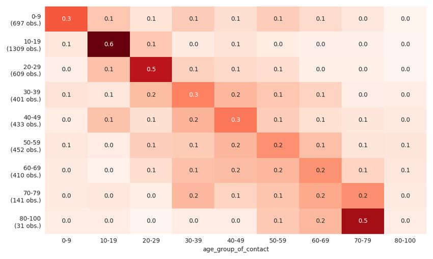
Figure 3. Distribution of random non-work contacts by age of participants.
Notes: The figure shows the distribution of random non-work contacts by age groups. A row shows the share
of contacts a certain age group has with all other age groups. Higher values are colored in darker red tones.
The diagonal represents the share of contacts with individuals from the same age group.
Figure 3 shows that assortativeness by age is especially strong for children and
younger adults. For older people, the pattern becomes more dispersed around their
own age group, but within-age-group contacts are still the most common contacts.
154.4 Infection Probabilities
To calibrate infection probabilities outside of the model, it would be important to
know the exact duration and distance of each contact type as well as viral loads.
Since this is not available in any dataset, we estimate those parameters inside the
model with the method of simulated moments (McFadden, 1989) by minimizing the
distance between simulated and observed infection rates. Since our model includes
a lot of randomness, we average simulated infection rates over several model runs.
Currently, we use data for Germany from August until November. We do not use
earlier periods to save computational time. Moreover, we would be worried that the
there are seasonal effects that we currently do not model.
To avoid overfitting and simplify the numerical optimization problem, we only
allow for four different probabilities: 1) for contacts in schools, preschools and nurs-
eries. 2) for work contacts. 3) for households. 4) for leisure activities.
4.5 Policies
In our empirical application we distinguish four groups of contact types: households,
education, work and other contacts. For households we assume that the individuals’
contacts in their households do not change over our estimation period. For nurs-
eries, preschools and schools we implement vacations as announced by the German
federal states as well as school closures. For the moment we ignore both emergency
childcare and that lack of childcare leads working parents to stay home. For our
work models⁷we use the reductions in work mobility reported in the Google Mobil-
ity Data (LLC, 2021) to calibrate our work policies. Reductions in work contacts are
not random but governed through a work contact priority where the policy changes
the threshold below which workers stay home. Figure 4 shows the share of workers
that go to work in our model over time.
Figure 4. Share of workers attending work normally.
Notes: The figure shows the percentage of pre-pandemic work mobility taking place since the start of the
pandemic. In our model this is used as a proxy for the share of workers that attend work as usual. Workers are
ordered with the importance of personal contacts for their work. Thus, if the share of
16For the last group of contacts which cover things like leisure activities, grocery
shopping etc. we have no reliable data by how much policies reduce them. In addi-
tion, they are likely to be affected by social and psychological factors such as pan-
demic fatigue and vacations. Because of this we estimate them like the infection
probabilities to fit the time series data. We use very few change points and tie them
to particular events such as policy announcements or particular holidays.
5 Model Validation
We validate our model in two ways: 1) We look at the in-sample fit over the esti-
mation period. 2) We look at the out-of-sample fit for November. The last one is a
challenging test for our model because there was a strong policy change between
the estimation period and November. The model convincingly passes both tests.
5.1 In-Sample Fit
Despite fitting only four infection probabilities, the in-sample fit is very good. The
best fit is achieved in the largest age groups. This is so mechanically, because we
weigh the deviations between simulated and observed infection rates by group sizes.
The worst fit is achieved for the 80 to 100 years old. There are three reasons for
this: Firstly, we only model private households at the moment, meaning that nurs-
ing homes are not part of the synthetic population we simulate. Since community
housing residents are part of the German Mikrozensus (Forschungsdatenzentren
Der Statistischen Ämter Des Bundes Und Der Länder, 2018) which forms the basis
for our synthetic population, we can and plan to include community housing res-
idents in the near future. Secondly, the elderly, especially nursing home residents,
are tested more often than the general population leading to more cases being de-
tected in this age group. We are currently working to include age-variant testing
strategies, using data by the RKI (Seifried and Hamouda, 2020).
7. We distinguish non-recurrent work contacts, daily work contacts and weekly work contacts.
17Figure 5. Reported vs. simulated weekly incidence rates of infections.
Notes: The figure shows the weekly incidence rates per 100,000 people for the reported (red line) versus the
simulated infections rates (blue line) for age groups available in the data provided by the Robert-Koch Institut.
5.2 Out-of-Sample Fit
We can assess the out-of-sample fit by projecting the effect of the lockdown light
and comparing it to case numbers until mid of November. It is important to note
that this is not just a simple extrapolation of a time trend because the lockdown
light only started after the estimation period. The out-of-sample fit can be assessed
in Figure 6.
The model correctly predicts the effect of the lockdown light with reasonable
accuracy. In particular, the actual case numbers are between our neutral and pes-
simistic projection. The plot also shows that ending the lockdown light on November
30, as was originally planned, would lead to an explosive growth in case numbers
in all scenarios.
18Figure 6. Predicted effect of the "Lockdown Light" on infection rates.
Notes: For the time period until the beginning of November, the figure shows the weekly incidence rates of
infections per 100,000 people from reported (black) versus simulated (blue) data. With the start of November,
the projections of the three scenarios, optimistic (blue), neutral (red), and pessimistic (mint green), are shown
until the beginning of the Christmas holidays. The actual incidence rates (black) are reported until the 24th
November.
6 Conclusion
We propose a simulation based model of infectious disease transmission that is de-
signed to predict the effects of fine-grained social distancing policies. In particular,
the model can be used to model policies such as several ways of splitting school
classes or work reduction policies that affect essential and non-essential workers
differentially. Both policies would be hard to implement in standard SEIR or agent
based simulation models.
To predict the effects of such policies, it is not only important to have a way of
expressing such flexible policies in terms of model quantities, but also to incorpo-
rate heterogeneity in disease progression as well as meeting patterns. We calibrate
age dependent disease progression parameters from the medical literature and age
dependent contact frequencies from contact diaries. Moreover, we distinguish ten
types of contacts out of which some are only relevant for certain age groups.
The model has a good fit on past German case numbers and passes an out of
sample validation despite a drastic change in the policy environment between the
estimation period and the validation period.
Despite these encouraging results we still see the model as work in progress. We
plan to implement more features, in particular allowing age and symptoms to affect
the probability to seek and receive a test, opening the way to show the effect of
different testing policies, such as those proposed by Tröger et al. (2020). Moreover,
19the estimation of the infection probabilities and the model fit will improve as more
data becomes available.
We invite researchers from any discipline, but particularly epidemiologists to
provide feedback on the model and welcome collaborations.
20References
Acemoglu, Daron, Victor Chernozhukov, Iván Werning, and Michael D Whinston. 2020. “Optimal
Targeted Lockdowns in a Multi-Group SIR Model.” Working Paper 27102. National Bureau of
Economic Research. DOI: 10.3386/w27102. [2]
Anderson, Elizabeth L., Paul Turnham, John R. Griffin, and Chester C. Clarke. 2020. “Consideration
of the Aerosol Transmission for COVID-19 and Public Health.” Risk Analysis 40 (5): 902–7. DOI:
10.1111/risa.13500. [8]
Avery, Christopher, William Bossert, Adam Clark, Glenn Ellison, and Sara Fisher Ellison. 2020. “An
Economist’s Guide to Epidemiology Models of Infectious Disease.” Journal of Economic Per-
spectives 34 (4): 79–104. DOI: 10.1257/jep.34.4.79. [2]
Berger, David W, Kyle F Herkenhoff, and Simon Mongey. 2020. “An SEIR Infectious Disease Model
with Testing and Conditional Quarantine.” Working Paper 26901. National Bureau of Economic
Research. DOI: 10.3386/w26901. [2]
Bi, Qifang, Yongsheng Wu, Shujiang Mei, Chenfei Ye, Xuan Zou, Zhen Zhang, Xiaojian Liu, Lan Wei,
Shaun A. Truelove, Tong Zhang, Wei Gao, Cong Cheng, Xiujuan Tang, Xiaoliang Wu, Yu Wu, Bin-
bin Sun, Suli Huang, Yu Sun, Juncen Zhang, Ting Ma, Justin Lessler, and Tiejian Feng. 2020.
“Epidemiology and Transmission of COVID-19 in Shenzhen China: Analysis of 391 cases and
1,286 of their close contacts.” (3): DOI: 10.1101/2020.03.03.20028423. [13]
Byrne, Andrew William, David McEvoy, Aine B Collins, Kevin Hunt, Miriam Casey, Ann Barber, Francis
Butler, John Griffin, Elizabeth A Lane, Conor McAloon, Kirsty O’Brien, Patrick Wall, Kieran A
Walsh, and Simon J More. 2020. “Inferred duration of infectious period of SARS-CoV-2: rapid
scoping review and analysis of available evidence for asymptomatic and symptomatic COVID-
19 cases.” BMJ Open 10 (8): e039856. DOI: 10.1136/bmjopen-2020-039856. [13]
Chen, Jun, Tangkai Qi, Li Liu, Yun Ling, Zhiping Qian, Tao Li, Feng Li, Qingnian Xu, Yuyi Zhang,
Shuibao Xu, Zhigang Song, Yigang Zeng, Yinzhong Shen, Yuxin Shi, Tongyu Zhu, and Hongzhou
Lu. 2020. “Clinical progression of patients with COVID-19 in Shanghai, China.” Journal of Infec-
tion 80 (5): e1–e6. DOI: 10.1016/j.jinf.2020.03.004. [14]
Cuevas, Erik. 2020. “An agent-based model to evaluate the COVID-19 transmission risks in facili-
ties.” Computers in Biology and Medicine 121 (6): 103827. DOI: 10.1016/j.compbiomed.2020.
103827. [3]
Donsimoni, Jean Roch, René Glawion, Bodo Plachter, and Klaus Wälde. 2020. “Projecting the spread
of COVID-19 for Germany.” German Economic Review 21 (2): 181–216. DOI: https://doi.org/10.
1515/ger-2020-0031. [2, 10]
Dorn, Florian, Janos Gabler, Hans-Martin von Gaudecker, Andreas Peichl, Tobias Raabe, and Klara
Rörhl. 2020. “Wenn Menschen (keine) Menschen treffen: Simulation der Auswirkungen von Poli-
tikmaßnahmen zur Eindämmung der zweiten Covid-19-Welle.” ifo Schnelldienst Digital, URL:
https://www.ifo.de/publikationen/ifo-schnelldienst. [2]
Dorn, Florian, Sahamoddin Khailaie, Marc Stöckli, Sebastian Binder, Berit Lange, Patrizio Vanella,
Timo Wollmershäuser, Andreas Peichl, Clemens Fuest, and Michael Meyer-Hermann. 2020.
“Das gemeinsame Interesse von Gesundheit und Wirtschaft: Eine Szenarienrechnung zur
Eindämmung der Corona- Pandemie.” ger. ifo Schnelldienst Digital 1 (6): URL: http://hdl.
handle.net/10419/223322. [2]
Duong, Diana. 2021. “What’s important to know about the new COVID-19 variants?” Canadian Med-
ical Association Journal 193 (4): E141–E142. DOI: 10.1503/cmaj.1095915. [1]
Forschungsdatenzentren Der Statistischen Ämter Des Bundes Und Der Länder. 2018. “Mikrozensus
2010, CF, Version 0.” de. DOI: 10.21242/12211.2010.00.00.5.1.0. [17]
Gabler, Janos, Tobias Raabe, Klara Röhrl, and Hans-Martin von Gaudecker. 2021. “Der Effekt von
Heimarbeit auf die Entwicklung der Covid-19-Pandemie in Deutschland.” Working paper. Insti-
21tute of Labor Economics (IZA). URL: https://www.iza.org/publications/s/100/der-effekt-von-
heimarbeit-auf-die-entwicklung-der-covid-19-pandemie-in-deutschland. [2]
Gabler, Janoś, Tobias Raabe, Klara Röhrl, and Hans-Martin von Gaudecker. 2020. “Die Be-
deutung individuellen Verhaltens über den Jahreswechsel für die Weiterentwicklung der
Covid-19-Pandemie in Deutschland.” Working paper. Institute of Labor Economics (IZA). URL:
https://www.iza.org/publications/s/99/die-bedeutung-individuellen-verhaltens-uber-den-
jahreswechsel-fur-die-weiterentwicklung-der-covid-19-pandemie-in-deutschland. [2, 8]
Gaythorpe, K, N Imai, G Cuomo-Dannenburg, M Baguelin, S Bhatia, A Boonyasiri, A Cori, Z Cucunuba
Perez, A Dighe, I Dorigatti, R Fitzjohn, H Fu, W Green, J Griffin, A Hamlet, W Hinsley, N Hong, M
Kwun, D Laydon, G Nedjati Gilani, L Okell, S Riley, H Thompson, S Van Elsland, R Verity, E Volz,
P Walker, H Wang, Y Wang, C Walters, C Whittaker, P Winskill, X Xi, C Donnelly, A Ghani, and
N Ferguson. 2020. “Report 8: Symptom progression of COVID-19.” DOI: 10.25561/77344. [14]
Grimm, Veronika, Friederike Mengel, and Martin Schmidt. 2020. “Extensions of the SEIR Model for
the Analysis of Tailored Social Distancing and Tracing Approaches to Cope with COVID-19.”
medRxiv, DOI: 10.1101/2020.04.24.20078113. eprint: https : // www . medrxiv . org / content /
early/2020/04/29/2020.04.24.20078113.full.pdf. [2]
He, Xi, Eric HY Lau, Peng Wu, Xilong Deng, Jian Wang, Xinxin Hao, Yiu Chung Lau, Jessica Y Wong, Yu-
juan Guan, Xinghua Tan, et al. 2020. “Temporal dynamics in viral shedding and transmissibility
of COVID-19.” Nature medicine 26 (5): 672–75. [9, 13]
Hinch, Robert, William J M Probert, Anel Nurtay, Michelle Kendall, Chris Wymatt, Matthew Hall, Ka-
trina Lythgoe, Ana Bulas Cruz, Lele Zhao, Andrea Stewart, Luca Ferritti, Daniel Montero, James
Warren, Nicole Mather, Matthew Abueg, Neo Wu, Anthony Finkelstein, David G Bonsall, Lucie
Abeler-Dorner, and Christophe Fraser. 2020. “OpenABM-Covid19 - an agent-based model for
non-pharmaceutical interventions against COVID-19 including contact tracing.” (9): DOI: 10.
1101/2020.09.16.20195925. [3]
LLC, Google. 2021. “Google COVID-19 Community Mobility Reports.” Working paper. URL: https://
www.google.com/covid19/mobility/. [16]
McAloon, Conor, Áine Collins, Kevin Hunt, Ann Barber, Andrew W Byrne, Francis Butler, Miriam
Casey, John Griffin, Elizabeth Lane, David McEvoy, Patrick Wall, Martin Green, Luke O’Grady,
and Simon J More. 2020. “Incubation period of COVID-19: a rapid systematic review and meta-
analysis of observational research.” BMJ Open 10 (8): e039652. DOI: 10.1136/bmjopen-2020-
039652. [12]
McFadden, Daniel. 1989. “A method of simulated moments for estimation of discrete response
models without numerical integration.” Econometrica: Journal of the Econometric Society, 995–
1026. [5, 16]
Morawska, Lidia, Julian W. Tang, William Bahnfleth, Philomena M. Bluyssen, Atze Boerstra, Giorgio
Buonanno, Junji Cao, Stephanie Dancer, Andres Floto, Francesco Franchimon, Charles Haworth,
Jaap Hogeling, Christina Isaxon, Jose L. Jimenez, Jarek Kurnitski, Yuguo Li, Marcel Loomans, Guy
Marks, Linsey C. Marr, Livio Mazzarella, Arsen Krikor Melikov, Shelly Miller, Donald K. Milton,
William Nazaroff, Peter V. Nielsen, Catherine Noakes, Jordan Peccia, Xavier Querol, Chandra
Sekhar, Olli Seppänen, Shin-ichi Tanabe, Raymond Tellier, Kwok Wai Tham, Pawel Wargocki,
Aneta Wierzbicka, and Maosheng Yao. 2020. “How can airborne transmission of COVID-19 in-
doors be minimised?” Environment International 142 (9): 105832. DOI: 10.1016/j.envint.2020.
105832. [8]
Mossong, Joël, Niel Hens, Mark Jit, Philippe Beutels, Kari Auranen, Rafael Mikolajczyk, Marco Mas-
sari, Stefania Salmaso, Gianpaolo Scalia Tomba, Jacco Wallinga, et al. 2008. “Social contacts
and mixing patterns relevant to the spread of infectious diseases.” PLoS medicine 5 (3): [4, 6,
15]
22Peak, Corey M, Rebecca Kahn, Yonatan H Grad, Lauren M Childs, Ruoran Li, Marc Lipsitch, and Car-
oline O Buckee. 2020. “Individual quarantine versus active monitoring of contacts for the mit-
igation of COVID-19: a modelling study.” Lancet Infectious Diseases 20 (9): 1025–33. DOI: 10.
1016/s1473-3099(20)30361-3. [13]
Priesemann, Viola, Melanie M Brinkmann, Sandra Ciesek, Sarah Cuschieri, Thomas Czypionka, Giu-
lia Giordano, Deepti Gurdasani, Claudia Hanson, Niel Hens, Emil Iftekhar, Michelle Kelly-Irving,
Peter Klimek, Mirjam Kretzschmar, Andreas Peichl, Matjaž Perc, Francesco Sannino, Eva Sch-
ernhammer, Alexander Schmidt, Anthony Staines, and Ewa Szczurek. 2021. “Calling for pan-
European commitment for rapid and sustained reduction in SARS-CoV-2 infections.” Lancet
397 (10269): 92–93. DOI: 10.1016/s0140-6736(20)32625-8. [1]
Seifried, Janna, and Osamah Hamouda. 2020. “Erfassung der SARS-CoV-2-Testzahlen in Deutsch-
land.” de. DOI: 10.25646/6634.2. [17]
Silva, Petrônio C.L., Paulo V.C. Batista, Hélder S. Lima, Marcos A. Alves, Frederico G. Guimarães, and
Rodrigo C.P. Silva. 2020. “COVID-ABS: An agent-based model of COVID-19 epidemic to simulate
health and economic effects of social distancing interventions.” Chaos, Solitons & Fractals
139 (10): 110088. DOI: 10.1016/j.chaos.2020.110088. [3]
Singanayagam, Anika, Monika Patel, Andre Charlett, Jamie Lopez Bernal, Vanessa Saliba, Joanna
Ellis, Shamez Ladhani, Maria Zambon, and Robin Gopal. 2020. “Duration of infectiousness and
correlation with RT-PCR cycle threshold values in cases of COVID-19, England, January to May
2020.” Eurosurveillance 25 (32): DOI: 10.2807/1560-7917.es.2020.25.32.2001483. [13]
Stokes, Erin K., Laura D. Zambrano, Kayla N. Anderson, Ellyn P. Marder, Kala M. Raz, Suad El Burai Fe-
lix, Yunfeng Tie, and Kathleen E. Fullerton. 2020. “Coronavirus Disease 2019 Case Surveillance
— United States, January 22–May 30, 2020.” MMWR. Morbidity and Mortality Weekly Report
69 (24): 759–65. DOI: 10.15585/mmwr.mm6924e2. [14]
Tröger, Thomas et al. 2020. “Optimal Testing and Social Distancing of Individuals With Private
Health Signals.” Working paper. University of Bonn, and University of Mannheim, Germany.
URL: https://www.crctr224.de/en/research-output/discussion-papers/archive/2020/DP229.
[4, 19]
Yin, Guosheng, and Huaqing Jin. 2020. “Comparison of Transmissibility of Coronavirus Between
Symptomatic and Asymptomatic Patients: Reanalysis of the Ningbo COVID-19 Data.” JMIR Pub-
lic Health and Surveillance 6 (2): e19464. DOI: 10.2196/19464. [13]
Zou, Lirong, Feng Ruan, Mingxing Huang, Lijun Liang, Huitao Huang, Zhongsi Hong, Jianxiang Yu,
Min Kang, Yingchao Song, Jinyu Xia, Qianfang Guo, Tie Song, Jianfeng He, Hui-Ling Yen, Malik
Peiris, and Jie Wu. 2020. “SARS-CoV-2 Viral Load in Upper Respiratory Specimens of Infected
Patients.” New England Journal of Medicine 382 (12): 1177–79. DOI: 10.1056/nejmc2001737.
[13]
23You can also read