Aerosol sources in the western Mediterranean during summertime: a model-based approach - Atmos. Chem. Phys
←
→
Page content transcription
If your browser does not render page correctly, please read the page content below
Atmos. Chem. Phys., 18, 9631–9659, 2018
https://doi.org/10.5194/acp-18-9631-2018
© Author(s) 2018. This work is distributed under
the Creative Commons Attribution 4.0 License.

Aerosol sources in the western Mediterranean during summertime:
a model-based approach
Mounir Chrit1 , Karine Sartelet1 , Jean Sciare2,6 , Jorge Pey3,a , José B. Nicolas4 , Nicolas Marchand 3 , Evelyn Freney4 ,
Karine Sellegri4 , Matthias Beekmann5 , and François Dulac2
1 CEREA,   joint laboratory Ecole des Ponts ParisTech – EDF R&D, Université Paris-Est, 77455 Champs-sur-Marne, France
2 LSCE,  CNRS-CEA-UVSQ,IPSL,Université Paris Saclay, Gif-sur-Yvette, France
3 Aix Marseille University-CNRS, LCE, Marseille, France
4 LAMP, UMR CNRS-Université Blaise Pascal, OPGC, Aubière, France
5 LISA, UMR 7583, Université Paris Diderot-Université Paris-Est Créteil, IPSL, Créteil, France
6 EEWRC, The Cyprus Institute, Nicosia, Cyprus
a now at the Spanish Geological Survey, IGME, 50006 Zaragoza, Spain

Correspondence: Mounir Chrit (mounir.chrit@enpc.fr)

Received: 3 October 2017 – Discussion started: 3 January 2018
Revised: 13 June 2018 – Accepted: 20 June 2018 – Published: 9 July 2018

Abstract. In the framework of ChArMEx (the Chemistry-              concentrations, a parameterization with an adequate wind
Aerosol Mediterranean Experiment), the air quality model           speed power law is chosen. Sulfate is shown to be strongly
Polyphemus is used to understand the sources of inorganic          influenced by anthropogenic (ship) emissions. PM10 , PM1 ,
and organic particles in the western Mediterranean and eval-       OM1 and sulfate concentrations are better described using
uate the uncertainties linked to the model parameters (mete-       the emission inventory with the best spatial description of
orological fields, anthropogenic and sea-salt emissions and        ship emissions (EDGAR-HTAP). However, this is not true
hypotheses related to the model representation of conden-          for nitrate, ammonium and chloride concentrations, which
sation/evaporation). The model is evaluated by comparisons         are very dependent on the hypotheses used in the model re-
to in situ aerosol measurements performed during three             garding condensation/evaporation. Model simulations show
consecutive summers (2012, 2013 and 2014). The model-              that sea-salt aerosols above the sea are not mixed with back-
to-measurement comparisons concern the concentrations of           ground transported aerosols. Taking the mixing state of par-
PM10 , PM1 , organic matter in PM1 (OM1 ) and inorganic            ticles with a dynamic approach to condensation/evaporation
aerosol concentrations monitored at a remote site (Ersa) on        into account may be necessary to accurately represent inor-
Corsica Island, as well as airborne measurements performed         ganic aerosol concentrations.
above the western Mediterranean Sea. Organic particles are
mostly from biogenic origin. The model parameterization of
sea-salt emissions has been shown to strongly influence the
concentrations of all particulate species (PM10 , PM1 , OM1        1   Introduction
and inorganic concentrations). Although the emission of or-
ganic matter by the sea has been shown to be low, organic          Fine particulate matter (PM) in the atmosphere is of concern
concentrations are influenced by sea-salt emissions; this is       due to its effects on health, climate, ecosystems and biolog-
owing to the fact that they provide a mass onto which gaseous      ical cycles, and visibility. These effects are especially im-
hydrophilic organic compounds can condense. PM10 , PM1 ,           portant in the Mediterranean region. The western Mediter-
OM1 are also very sensitive to meteorology, which affects          ranean basin experiences high gaseous pollution levels origi-
not only the transport of pollutants but also natural emissions    nating from Europe (Millán et al., 1997; Debevec et al., 2017;
(biogenic and sea salt). To avoid large and unrealistic sea-salt   Doche et al., 2014; Menut et al., 2015; Nabat et al., 2013;
                                                                   Safieddine et al., 2014) in particular during summer, when

Published by Copernicus Publications on behalf of the European Geosciences Union.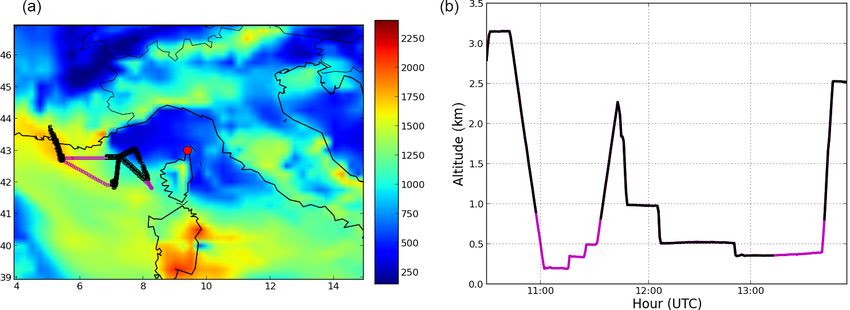
9632                                    M. Chrit et al.: Aerosol sources in the western Mediterranean during summertime

photochemical activity is at its maximum. Furthermore, the         pogenic emissions, uncertainties concern not only the emis-
western Mediterranean basin is impacted by various natural         sions themselves, but also the pollutants that are to be con-
sources: Saharan dust, intense biogenic emissions in summer,       sidered in the inventory and the spatial and temporal dis-
oceanic emissions and biomass burning, all of which emit           tributions of the emissions. For example, intermediate and
gases (e.g., volatile organic compounds (VOC), nitrogen ox-        semi-volatile organic compounds are missing from emission
ides (NOx )) and/or primary particles (Bossioli et al., 2016;      inventories, even though they may strongly affect the forma-
Tyrlis and Lelieveld, 2012; Monks et al., 2009; Gerasopou-         tion of organic aerosols (Couvidat et al., 2012; Denier van der
los et al., 2006). During the TRAQA 2012 and SAFMED                Gon et al., 2015). The spatial distribution of ships and harbor
2013 measurement campaigns, Di Biagio et al. (2015) ob-            traffic differs depending on emission inventories; however,
served that aerosols in the western Mediterranean basin are        over the Mediterranean Sea, ships and harbor traffic emis-
strongly impacted by dust outflows and continental pollution.      sions may strongly affect the formation of particles. Becagli
A large part of this continental pollution is secondary, i.e.,     et al. (2017) found that the minimum ship emission contri-
it is formed in the atmosphere by chemical reactions (e.g.,        butions to PM10 were 11 % at Lampedusa Island, and 8 %
Sartelet et al., 2012). These reactions involve compounds,         at Capo Granitola on the southern coast of Sicily. Aksoyoglu
which may be emitted from different sources (e.g., biogenic        et al. (2016) showed that ship emissions in the Mediterranean
and anthropogenic). Using measurements and/or modeling,            may contribute up to 60 % of sulfate concentrations, as SO2
several studies have shown that as much as 70 to 80 % of           is a major pollutant emitted from maritime transport. How-
organic aerosol in summer in the western Mediterranean re-         ever, in comparison to on-road vehicles, ship emissions are
gion is secondary and from contemporary origins (El Haddad         still poorly characterized (Berg et al., 2012). Furthermore,
et al., 2011; Chrit et al., 2017).                                 the multiplicity of Mediterranean pollution sources and their
   Air quality models are powerful tools to simulate and pre-      interactions makes it difficult to quantify ship contributions
dict the atmospheric chemical composition and the proper-          to aerosol concentrations.
ties of aerosols at regional scales. In spite of the tremendous       Seas and oceans are a significant source of sea-spray
efforts made recently, the sources and transformation mecha-       aerosols (SSA), which strongly affect the formation of cloud
nisms of atmospheric aerosols are not fully characterized nor      condensation nuclei and particle concentrations. However,
fully understood. For organic aerosols, modeling difficulties      according to Grythe et al. (2014), sea-spray aerosols (SSA)
partly lie in the representation of volatile and semi-volatile     have one of the largest uncertainties among all emissions.
organic precursors, which can only take a limited number of        The modeling of sea-salt emissions is based on empirical or
compounds or classes of compounds into account(Kim et al.,         semi-empirical formulas. There is a tremendous amount of
2011a; Chrit et al., 2017). Difficulties in modeling atmo-         parameterization of the SSA emission fluxes (Grythe et al.,
spheric particles are strongly linked to uncertainties in me-      2014). The SSA emission parameterization of Monahan et al.
teorology and emissions (Roustan et al., 2010). For example,       (1986) is commonly used to model sea-salt emissions of
turbulent vertical mixing affects the dilution and chemical        coarse particles (e.g., Sartelet et al., 2012; Solazzo et al.,
processing of aerosols and their precursors (Nilsson et al.,       2017; Kim et al., 2017). However, the strong non-linearity
2001; Aan de Brugh et al., 2012), clouds affect aerosol chem-      of the source function versus wind speed (power law with an
istry and size distribution (Fahey and Pandis, 2001; Ervens        exponent of 3.41) may lead to an overestimation of emissions
et al., 2011) and photochemistry (Tang et al., 2003; Feng          at high-speed regimes, as suggested by Guelle et al. (2001)
et al., 2004), and precipitation controls wet deposition pro-      and Witek et al. (2007). Many studies have shown that wind
cesses (Barth et al., 2007; Yang et al., 2012; Wang et al.,        speed is the dominant influence on sea-salt emissions (Hop-
2013). Over the Mediterranean region, uncertainties due to         pel et al., 1989; Grythe et al., 2014). However, other parame-
meteorology and transport may strongly impact pollutant            terizations use different power laws with different exponents
concentrations. This is due to the fact that the basin is influ-   for the wind speed (e.g., 2.07 for Jaeglé et al., 2011) and
enced by pollution transported from different regions, such        have introduced other parameters like sea-surface tempera-
as dust from Algeria, Tunisia and Morocco as well as both          ture (Schwier et al., 2017; Jaeglé et al., 2011; Sofiev et al.,
biogenic and anthropogenic species from Europe (Chrit et al.,      2011) and water salinity (Grythe et al., 2014). Although the
2017; Denjean et al., 2016). Chrit et al. (2017) and Cholakian     influence of marine emissions on primary organic aerosols is
et al. (2018) have shown that although organic aerosol con-        low for the Mediterranean (Chrit et al., 2017), their influence
centrations at a remote marine site in the western Mediter-        on inorganic aerosols is not (Claeys et al., 2017).
ranean are mostly of biogenic origin, they are strongly influ-        The aim of this work is to evaluate some of the processes
enced by air masses transported from the continent and by          that strongly affect inorganic and organic aerosol concentra-
maritime shipping emissions.                                       tions in the western Mediterranean in summer (transport and
   In addition to the meteorological uncertainties, uncertain-     emissions), and to establish how the data/parameterizations
ties in emission inventories are also important. There are un-     commonly used in air quality models affect the concentra-
certainties in biogenic emissions (Sartelet et al., 2012), as      tions. To that end, sensitivity studies relative to transport
well as in anthropogenic emission inventories. For anthro-         (meteorology) and emissions (anthropogenic and sea salt)

Atmos. Chem. Phys., 18, 9631–9659, 2018                                             www.atmos-chem-phys.net/18/9631/2018/
M. Chrit et al.: Aerosol sources in the western Mediterranean during summertime                                                        9633

Figure 1. Mediterranean domain used for the simulations and planetary boundary layer (PBL) height on 10 July 2014 at noon, as obtained
from the ECMWF meteorological fields (a). Ersa is located at the red point on northern tip of Corsica Island. The (black and purple)
crosses/lines indicate the trajectory of the flight on 10 July 2014 over the Mediterranean Sea. The altitudes during the flight are displayed
in (b). The portions conducted above the continent at the beginning and at the end of the flight from/to Avignon airport have been removed.
For the model-to-measurement comparisons, only the transects indicated by purple crosses/lines are considered.

are performed using the Polyphemus air quality model. The                2.1   Simulation setups and alternative
model results are then compared to measurements performed                      parameterizations
at the remote marine Ersa super-site (Cap Corsica, France)
during the summer campaigns of 2012 and 2013, and to air-
borne measurements performed above the Western Mediter-                  Simulations are performed over the same domains and using
ranean Sea in summer (July) 2014.                                        the same input data as in Chrit et al. (2017).
   This paper is structured as follows. The Polyphemus air                  Two nested simulations are performed: one over Eu-
quality model setup is first described for the different in-             rope (nesting domain, horizontal resolution: 0.5◦ × 0.5◦ ) and
put datasets/parameterizations used, as well as the measure-             one over a Mediterranean domain centered around Cor-
ments. Second, the meteorological fields used as input for the           sica (nested domain, horizontal resolution: 0.125◦ × 0.125◦ ),
air quality model are evaluated. Third, the model is evaluated           which is also centered around the Ersa surface super-site
by comparisons to the measurements and comparisons of the                (red point in Fig. 1). Vertically, 14 levels are used in Po-
sensitivities studies to meteorology, sea-salt emission param-           lair3d/Polyphemus. The heights of the cell interfaces are 0,
eterizations and anthropogenic emissions are performed to                30, 60, 100, 150, 200, 300, 500, 750, 1000, 1500, 2400, 3500,
determine the main aerosol sources and sensitivities.                    6000 and 12 000 m.
                                                                            Simulations are performed during the summers of 2012,
                                                                         2013 and 2014. The dates of simulations are chosen
2   Simulation setups and measured data                                  to match the periods of observations performed during
                                                                         ChArMEx (Chemistry-Aerosol Mediterranean Experiment).
In order to simulate aerosol formation over the western                  The Mediterranean simulations (nested domain) are per-
Mediterranean, the Polair3d/Polyphemus air quality model                 formed from 6 June to 8 July 2012, from 6 June to 10 August
is used, with the setup described in Chrit et al. (2017)                 2013 and from 9 to 10 July 2014. In the reference simula-
and summarized here. For parameters/parameterizations                    tion, meteorological data are provided by the European Cen-
that are particularly related to uncertainties (anthropogenic            ter for Medium-Range Weather Forecasts (ECMWF) model
emissions, meteorology, sea-salt emissions and model-                    (horizontal resolution: 0.25◦ × 0.25◦ ), which are interpolated
ing of condensation/evaporation), the alternative parame-                to the Europe and Mediterranean study domains. The verti-
ters/parameterizations that are used in the sensitivity studies          cal diffusion is computed using the Troen and Mahrt (1986)
are also detailed for emissions and meteorology. For compu-              parameterization. In the sensitivity study relative to meteo-
tational reasons, alternative parameterizations for the model-           rology, meteorological fields from the Weather Research and
ing of condensation/evaporation are only used in the compar-             Forecasting model (WRF, Skamarock et al., 2008) are used
isons to airborne measurements in Sect. 4.4 (where they are              in the Mediterranean simulation. WRF is forced with NCEP
also detailed).                                                          (National Centers for Environmental Prediction) meteoro-
                                                                         logical fields for initial and boundary conditions (1◦ hori-
                                                                         zontal grid spacing). To simulate WRF meteorological fields

www.atmos-chem-phys.net/18/9631/2018/                                                      Atmos. Chem. Phys., 18, 9631–9659, 2018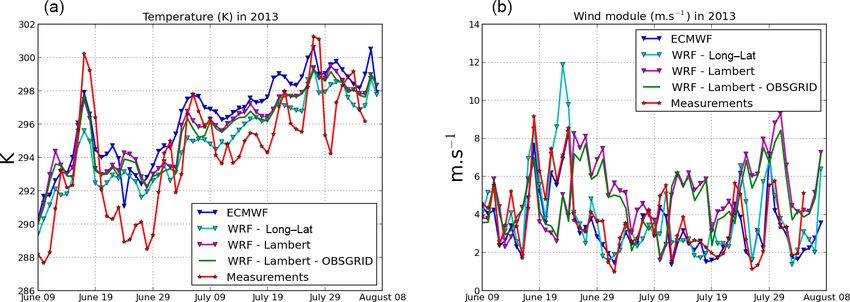
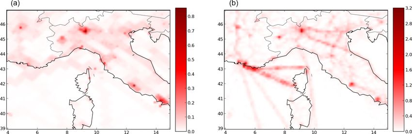
9634                                    M. Chrit et al.: Aerosol sources in the western Mediterranean during summertime

Figure 2. Average NOx emissions over the summer campaign 2013 from the EMEP emission inventory (a), and absolute differences
(µg m−2 s−1 ) of NOx emissions between HTAP and EMEP inventories (b). The horizontal and vertical axes show longitude and latitude in
degrees, respectively.

over the Mediterranean domain, one-way nested WRF sim-               cal data used for transport. In the reference simulation, yearly
ulations with 24 vertical levels are conducted on two nested         anthropogenic emissions are generated using the EDGAR-
domains: one over Europe and one over the Mediterranean.             HTAP_V2 inventory for 2010 (http://edgar.jrc.ec.europa.eu/
Before conducting the sensitivity study relative to meteorol-        htap_v2/). The EDGAR-HTAP_V2 inventory uses total na-
ogy (Sect. 3), using two different meteorological datasets,          tional emissions from the European Monitoring and Evalua-
WRF is run with a number of different configurations, which          tion Program (EMEP) emission inventory that are spatially
are compared to measurements in Sect. 3. In these configura-         reallocated using the EDGAR4.1 proxy subset (Janssens-
tions, the same physical parameterizations are used, but with        Maenhout et al., 2012). The differences between the two in-
different horizontal coordinates.                                    ventories do not only lie in the spatial allocation of emis-
   The WRF configuration used for this study consists of the         sions, but also in the spatial resolution. EMEP provides a
Single Moment-5 class microphysics scheme (Hong et al.,              resolution of 0.5◦ × 0.5◦ , while the resolution of EDGAR-
2004), the RRTM radiation scheme (Mlawer et al., 1997),              HTAP_V2 is 0.1◦ × 0.1◦ . To illustrate the differences be-
the Monin–Obukhov surface layer scheme (Janjic, 2003),               tween the two inventories, NOx emissions from the EMEP
and the NOAA land surface model scheme for land surface              emission inventory and absolute differences of NOx emis-
physics (Chen and Dudhia, 2001). Sea surface temperature             sions between the HTAP and EMEP inventories are shown in
update and surface grid nudging (Liu et al., 2012; Bowden            Fig. 2. The highest discrepancies between the two inventories
et al., 2012) options are activated.                                 mostly concern shipping emissions (very low in the EMEP
   In the first configuration (WRF-Lon-Lat), horizontal              emission inventory (< 0.2 µg m−2 s−1 ), whereas they can be
resolutions of 0.5◦ × 0.5◦ and 0.125◦ × 0.125◦ are used              as high as 2.8 µg m−2 s−1 over the sea in the HTAP emission
for the nesting and nested domains, respectively, with a             inventory) as well as for emissions over large cities, primar-
longitude–latitude projection. In the second configuration           ily Genoa, Marseille and Rome (with emissions as high as
(WRF-Lambert), a Lambert (conic conform) projection is               2.5 µg m−2 s−1 higher than in the HTAP emission inventory).
used with horizontal resolutions of 55.65 km × 55.65 km              HTAP emissions are used in the reference simulation and
and 13.9 km × 13.9 km for the nesting and nested do-                 EMEP emissions are used in the sensitivity study as shown
mains, respectively. The third configuration (WRF-Lambert-           in Table 1.
OBSGRID) also uses a Lambert projection, but the meteoro-               Sea-salt emissions are parameterized using Jaeglé et al.
logical fields are improved by nudging global observations of        (2011) in the reference simulation and utilizing the
temperature, humidity and wind from surface and radiosonde           commonly-used Monahan et al. (1986) parameterization for
measurements (NCEP operational global surface and upper-             the sensitivity study. These two parameterizations are based
air observation subsets, as archived by the Data Support Sec-        on open-sea measurements but are different in terms of the
tion (DSS) at NCAR (National Center for Atmospheric Re-              source function, which is defined as the total mass of sea-salt
search)).                                                            aerosol (SSA) released by area and time units. Furthermore,
   Biogenic emissions are estimated using MEGAN (Model               the source functions of these two parameterizations have a
of Emissions of Gases and Aerosols from Nature) with the             different dependency on the wind speed.
standard MEGAN LAIv database (MEGAN-L, Guenther                         In terms of emitted sea-salt mass, the largest differences
et al., 2006) and the EFv2.1 dataset. For the different simula-      are located over the sea in the south of France (with differ-
tions, these emissions are recalculated with the meteorologi-        ences as high as 1400 %), where the shear stress exerted by

Atmos. Chem. Phys., 18, 9631–9659, 2018                                               www.atmos-chem-phys.net/18/9631/2018/
M. Chrit et al.: Aerosol sources in the western Mediterranean during summertime                                                    9635

Table 1. Summary of the different simulations and their input data. S1, S2, S3, S4 and S5 represent the simulation number.

                                   Anthropogenic emission     Meteorological     Sea-salt emission        I/S-VOC/POA
                 Nomenclature
                                         inventory            model              parameterization
                 S1                         HTAP              ECMWF              Jaeglé et al. (2011)                1.5
                 S2                         HTAP              WRF Lon-Lat        Jaeglé et al. (2011)                1.5
                 S3                         HTAP              ECMWF              Monahan et al. (1986)               1.5
                 S4                         EMEP              ECMWF              Jaeglé et al. (2011)                1.5
                 S5                         HTAP              ECMWF              Jaeglé et al. (2011)                0.0

the wind on the sea surface is highest. Following Schwier               with absorption by the organic phase (hydrophobic surro-
et al. (2015), the emitted dry sea-salt mass is assumed to be           gates). The gas–particle partitioning of hydrophilic surro-
made up of 25.40 % chloride, 30.61 % sodium and 4.22 %                  gates is computed using Henry’s law modified to extrapo-
sulfate.                                                                late infinite dilution conditions to all conditions using an
    The boundary conditions for the European simulation are             aqueous-phase partitioning coefficient with absorption by the
calculated from the global model MOZART4 (Horowitz                      aqueous phase (hydrophilic organics, inorganics and water).
et al., 2003) (https://www.acom.ucar.edu/wrf-chem/mozart.               Activity coefficients are computed with the thermodynamic
shtml), whilst those for the Mediterranean domain are ob-               model UNIFAC (UNIversal Functional Activity Coefficient;
tained from the European simulation. Mineral dust emissions             (Fredenslund et al., 1975)). After condensation/evaporation,
are not calculated in the model, but are provided from the              the moving diameter algorithm is used for mass redistribu-
boundaries, and their heterogeneous reactions to form nitrate           tion among size bins. As detailed in Chrit et al. (2017), an-
and sulfate are not taken into account.                                 thropogenic intermediate/semi-volatile organic compounds’
    The numerical algorithms used for transport and the pa-             (I/S-VOC) emissions are emitted as three primary surrogates
rameterizations used for dry and wet depositions are detailed           of different volatilities (characterized by their saturation con-
in Sartelet et al. (2007). Gas-phase chemistry is modeled               centrations C∗ : log(C∗ ) = −0.04, 1.93 and 3.5). The ageing
with the carbon bond 05 mechanism (CB05) (Yarwood et al.,               of each primary surrogate is represented through a single
2005), to which reactions are added to model the formation              oxidation step, without NOx dependency, to produce a sec-
of secondary organic aerosols (Kim et al., 2011b; Chrit et al.,         ondary surrogate of lower volatility (log(C∗ ) = −2.4, −0.064
2017).                                                                  and 1.5, respectively) but higher molecular weight. Gaseous
    The Size Resolved Aerosol Model (SIREAM; Debry et al.,              I/S-VOC emissions are missing from emission inventories
2007) is used for simulating the dynamics of the aerosol size           and are estimated here as detailed in Zhu et al. (2016): by
distribution by coagulation and condensation/evaporation.               multiplying the primary organic emissions (POA) by 1.5, and
SIREAM uses a sectional approach and the aerosol dis-                   by assigning them to species of different volatilities. A sen-
tribution is described here using 20 sections of bound                  sitivity study where I-S/VOC emissions are not taken into
diameters: 0.01, 0.0141, 0.0199, 0.0281, 0.0398, 0.0562,                account is also performed.
0.0794, 0.1121, 0.1585, 0.2512, 0.3981, 0.6310, 1.0, 1.2589,               Sensitivity studies to meteorology fields, anthropogenic
1.5849, 1.9953, 2.5119, 3.5481, 5.0119, 7.0795 and 10.0 µm.             emission inventory, I/S-VOC emissions and sea-salt emis-
The condensation/evaporation of inorganic aerosols is deter-            sions are outlined in Sect. 4. These studies are performed
mined using the thermodynamic model ISORROPIA (Nenes                    using two different inputs for the parameter of interest in
et al., 1998) with a bulk equilibrium approach in order to              the sensitivity test and fixing the others. Table 1 summarizes
compute the partitioning between the gaseous and particle               the simulations performed as well as the different input data
phases of aerosols. Because the concentrations and the par-             used. Table 2 summarizes the different simulation compar-
titioning between gaseous and particle phases of chloride,              isons, as performed in the conducted sensitivity studies.
nitrate and ammonium are strongly affected by condensa-
tion/evaporation and reactions with other pollutants, sensi-            2.2    Measured data
tivities of these concentrations to the hypotheses used in
the modeling (thermodynamic equilibrium, mixed sea-salt                 The model results are compared against observational data
and anthropogenic aerosols) are also performed (Sect. 4.4.2).           collected in the framework of several ChArMEx campaigns.
For organic aerosols, the gas–particle partitioning of the              Simulated concentrations in the first vertical level of the
surrogates is computed using SOAP (Secondary Organic                    model are compared to ground-based measurements per-
Aerosol Processor), assuming bulk equilibrium (Couvidat                 formed at Ersa (43◦ 000 N, 9◦ 21.50 E), which is located on the
and Sartelet, 2015). The gas–particle partitioning of hy-               northern edge of Corsica Island, at a height of about 530 m
drophobic surrogates is modeled following Pankow (1994),                above sea level (Fig. 1). A Campbell meteorological station
                                                                        was used to measure air temperature and wind speed. Contin-

www.atmos-chem-phys.net/18/9631/2018/                                                     Atmos. Chem. Phys., 18, 9631–9659, 2018
9636                                      M. Chrit et al.: Aerosol sources in the western Mediterranean during summertime

Table 2. Summary of the different sensitivity simulations for the ground-based evaluation.

       Sensitivity study                   Compared simulations      Discussed concentrations             Period
       Meteorology                         S1 and S2                 Inorganics , PM10 , PM1 and OM1      Summer 2013
       Anthropogenic emission inventory    S1 and S4                 Inorganics , PM10 , PM1 and OM1      Summers 2012 and 2013
       Marine emissions                    S1 and S3                 Inorganics , PM10 , PM1 and OM1      Summer 2013
       I/S-VOC/POA                         S1 and S5                 OM1                                  Summer 2013

uous measurements of PM10 and PM1 were performed using                  perature and wind at Ersa in Fig. B1 for the summer cam-
TEOM (Thermo Scientific, model 1400) and TEOM-FDMS                      paign periods of 2012 and in Fig. B2 for the summer 2013
(Thermo Scientific, model 1405) instruments, respectively.              (Appendix B).
The composition of particles, nitrate, sulfate, ammonium and               The observed and simulated temperature, wind speed,
organic concentrations in PM1 were characterized using an               wind direction and relative humidity at Ersa during these
ACSM (aerosol chemical speciation monitor); in PM10 they                summers, the statistical scores defined in Table A1 of Ap-
were characterized using a PILS-IC (particle into liquid sam-           pendix A and the comparison of the four model results to
pler coupled with ion chromatography), which also allowed               measurements (hourly time series) are shown in Tables 3–6,
for an estimation of chloride and sodium concentrations (see            respectively.
Michoud et al., 2017 for more details). The inorganic precur-              As mentioned in the 2007 EPA report, Emery et al. (2001)
sors HNO3 , HCl and SO2 were measured using a WAD-IC                    proposed benchmarks for temperature (mean bias (MB)
(wet-annular denuder coupled with ion chromatography).                  within ±0.5 K and a gross error (GE) of 2.0 K), wind speed
   Airborne measurements based in Avignon, France were                  (MB within ±0.5 m s−1 and a RMSE < 2 m s−1 ) and wind di-
performed aboard the ATR-42, run by SAFIRE (French air-                 rection (MB within ±10◦ and a GE < 30◦ ). McNally (2009)
craft service for environmental research, http://safire.fr, last        suggested an alternative set of benchmarks for temperature
access: 4 July 2017). Full details of the aerosol measurements          (MB within ±1.0 K and a GE < 3.0 K).
aboard the aircraft as well as the flight details are provided             The four meteorological simulations reproduce the ground
in Freney et al. (2018). On 10 July 2014, a flight was dedi-            temperature measured at Ersa well. Whilst only the ECMWF
cated to measure concentrations above the sea under a “mis-             temperature in 2012 verifies the US EPA criteria, all simu-
tral” regime (northern and northwestern high-speed winds).              lations verify the criterion from McNally (2009) for the GE.
This flight was approximately 3 h in duration and the aircraft          Statistically, the correlation to temperature measurements is
flew over the south of France and the Mediterranean Sea at              high (between about 54 and 96 % for all models), and the
altitudes varying from 100 to 3000 meters above sea level               root mean square error (RMSE) is low (below 3.4 K). The
(m a.s.l). Comparisons between the model and the measure-               best model differs depending on the year: the correlation
ments are not performed during transit; they are only per-              of ECMWF to measurements is the highest (96 %) and the
formed above the sea at altitudes below 800 m a.s.l. and in             RMSE the lowest (1.5 K) in 2012, but in 2013, the correla-
the boundary layer. A horizontal projection of the aircraft             tion of ECMWF is the lowest (70 %) and its RMSE the high-
path during this flight is presented in Fig. 1. The purple              est (3.2 K). The mean fractional biases and errors (MFB and
crosses/lines indicate the locations where model and mea-               MBE) of the simulated temperatures are almost zero.
surement comparisons are performed. Measurements of the                    For wind speed, ECMWF systematically leads to bet-
non-refractory submicron aerosol chemical properties were               ter statistics than WRF, despite the fine horizontal resolu-
performed using a compact aerosol time-of-flight mass spec-             tion of WRF (0.125◦ × 0.125◦ ). ECMWF agrees best with
trometer (C-ToF-AMS) providing mass concentrations of or-               the measurements, with the highest correlation (between 69
ganic sulfate, ammonia and chloride particles with a time res-          and 87 %) and the lowest errors (MFE is between 33 and
olution of less than 5 min.                                             47 %). It also verifies the US EPA criteria for both the 2012
                                                                        and 2013 summers. WRF-Lon-Lat also performs well with
                                                                        correlations between 60 and 65 % and MFEs between 47
3   Meteorological evaluation                                           and 64 %. WRF-Lambert and WRF-Lambert-Obsgrid have
                                                                        poorer statistics with negative correlations and MFEs be-
Aerosol phenomenology on the Corsica Cape is influenced                 tween 71 and 74 %.
by diverse meteorological situations as well as transport of               The average wind direction is quite similar for the 2012
pollutants from a number of sources. Therefore, it is crucial           and 2013 summers (202 and 186◦ , respectively). The mean
to estimate the input meteorological data used in the air qual-         wind direction is best represented by ECMWF for the 2013
ity model as accurately as possible. The four meteorological            summer, and WRF-Lon-Lat for the 2012 summer. However,
datasets (ECMWF, WRF-Lon-Lat, WRF-Lambert and WRF-                      the modeled wind speed does not respect the US EPA crite-
Lambert-Obsgrid) are compared to observations of air tem-

Atmos. Chem. Phys., 18, 9631–9659, 2018                                                      www.atmos-chem-phys.net/18/9631/2018/
M. Chrit et al.: Aerosol sources in the western Mediterranean during summertime                                                          9637

Table 3. Temperature (observed and simulated means) from the observations and the four meteorological models at Ersa during the 2012 and
2013 summer campaigns, and statistics of comparison of model results to observations (correlation, mean fractional bias, mean fractional
error, mean bias and gross error). The temperature means and RMSEs are in Kelvin. o refers to the measured mean.

         Meteorological models                                   ECMWF       WRF-Lon-Lat      WRF-Lambert      WRF-Lambert-OBSGRID
                                  Simulated mean s ± RMSE    295.09 ± 1.50    294.05 ± 2.79    294.86 ± 3.02             294.17 ± 3.45
                  o = 294.66

                                  Correlation (%)                     96.3             77.1             66.7                      54.8
         2012

                                  MFB                                 0.00             0.00             0.00                      0.00
                                  MFE                                 0.00             0.01             0.01                      0.01
                                  MB                                  0.43           −0.61              0.20                    −0.49
                                  GE                                  1.33             2.38             2.56                      2.93
                                  Simulated mean s ± RMSE     295.82 ± 3.2    294.42 ± 2.42    295.31 ± 2.66             295.10 ± 2.60
                  o = 294.04

                                  Correlation (%)                     70.0             78.2             79.0                      78.3
         2013

                                  MFB                                 0.01             0.00             0.00                      0.00
                                  MFE                                 0.01             0.01             0.01                      0.01
                                  MB                                  1.79             0.38             1.27                      1.06
                                  GE                                  2.69             2.01             2.17                      2.14

Table 4. Wind speed statistics for the four meteorological models at Ersa during the 2012 and 2013 summer campaigns. The wind speed
means and the RMSEs are in m s−1 . o refers to the measured mean.

           Meteorological models                                ECMWF        WRF-Lon-Lat      WRF-Lambert      WRF-Lambert-OBSGRID
                                   Simulated mean s ± RMSE    4.86 ± 2.36      6.96 ± 3.93      5.60 ± 3.94               5.06 ± 3.89
                                   Correlation (%)                   69.3             60.3           −26.0                     −34.3
                       o = 4.53
           2012

                                   MFB                               0.14             0.46             0.34                      0.26
                                   MFE                               0.47             0.64             0.74                      0.74
                                   MB                                0.33             2.40             1.07                      0.52
                                   GE                                1.89             3.28             3.45                      3.34
                                   Simulated mean s ± RMSE    3.44 ± 1.32      3.98 ± 2.12      5.14 ± 3.64               4.86 ± 3.44
                                   Correlation (%)                   87.3             65.5            −6.6                      −2.1
                       o = 3.21
           2013

                                   MFB                               0.01             0.10             0.38                      0.30
                                   MFE                               0.33             0.47             0.73                      0.71
                                   MB                              −0.35              0.19             1.36                      1.07
                                   GE                                1.01             1.59             3.06                      2.88

ria. Errors are higher with the two models using the Lambert                      summer 2013 (not exactly the same period – 10 July to 5 Au-
projection, which tend to underestimate the wind direction                        gust 2013), Cholakian et al. (2018) found a RMSE between
angle. For relative humidity, the observed mean relative hu-                      1.5 and 2.3 K for temperature, between 1.6 and 1.9 m s−1 for
midity is 0.65 in 2012 and 0.70 in 2013. It is relatively well                    wind speed and between 92 and 117◦ for wind direction us-
reproduced by the models (between 0.70 and 0.77 in 2012                           ing the mesoscale WRF model. Moreover, Kim et al. (2013)
and between 0.69 and 0.78 in 2013). All models perform well                       reported a RMSE ranging between 1 and 4 K for tempera-
with a MFE below 32 % and a MFB below 18 %. WRF-Lon-                              ture, and 0.6 to 3.0 m s−1 for wind speed over Greater Paris
Lat leads to the best statistics in 2012 and WRF-Lambert-                         during May 2005 using the WRF model with a longitude–
Obsgrid leads to the best statistics in 2013.                                     latitude map projection.
   As ECMWF and WRF-Lon-Lat show better overall per-
formance than the other two models (Tables 3–6), they are
used for the meteorological sensitivity study.                                    4   Evaluation and sensitivities
   The model performances presented above compare well to
other studies (Kim et al., 2013; Cholakian et al., 2018). In this                 This section focuses on the evaluation of the reference simu-
study, for ECMWF and WRF-Lon-Lat during the summers                               lation (S1) against aerosol measurements (PM10 , PM1 , OM1
of 2012 and 2013, the RMSE ranges between 1.5 and 3.2 K                           and inorganic aerosols (IA) species), in addition to the fac-
for temperature, between 1.3 and 3.9 m s−1 for wind speed                         tors controlling simulated aerosol concentrations (meteorol-
and between 58 and 118◦ for wind direction. At Ersa, for the                      ogy, sea-salt and anthropogenic emissions). This evaluation
                                                                                  is performed against ground-based measurements during the

www.atmos-chem-phys.net/18/9631/2018/                                                              Atmos. Chem. Phys., 18, 9631–9659, 2018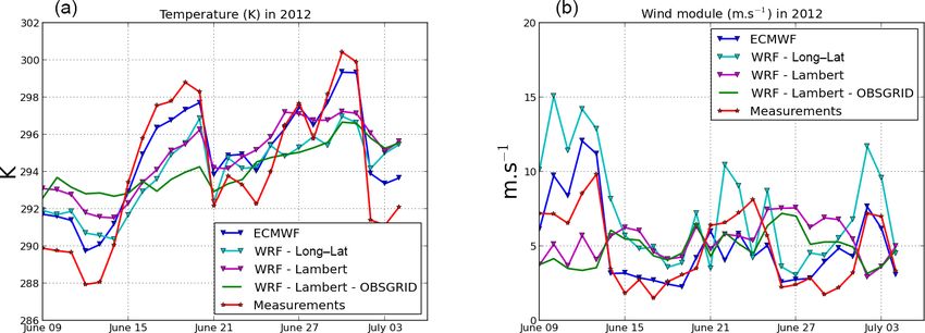
9638 M. Chrit et al.: Aerosol sources in the western Mediterranean during summertime
Table 5. Wind direction statistics for the four meteorological models at Ersa during the 2012 and 2013 summer campaigns. The wind
direction means and the RMSEs are in degrees. o refers to the measured mean.
Meteorological models ECMWF WRF-Lon-Lat WRF-Lambert WRF-Lambert-OBSGRID
Simulated mean s ± RMSE 195.73 ± 91.64 200.48 ± 58.94 107.07 ± 120.47 101.30 ± 119.53
o = 201.89
Correlation (%) 27.6 54.1 7.2 12.0
2012
MFB −0.14 −0.02 −0.62 −0.66
MFE 0.40 0.22 0.68 0.69
MB −6.16 −1.41 −94.82 −100.59
GE 62.09 39.74 104.00 104.43
Simulated mean s ± RMSE 206.67 ± 107.84 231.03 ± 117.91 101.57 ± 120.47 111.46 ± 122.76
o = 186.28
Correlation (%) 33.2 21.6 3.6 1.7
2013
MFB −0.02 0.13 −0.50 −0.48
MFE 0.48 0.46 0.67 0.68
MB 20.38 44.74 −84.71 −74.83
GE 73.96 81.34 100.13 101.88
Table 6. Relative humidity statistics for the four meteorological models at Ersa during the 2012 and 2013 summers. The relative humidity
means and the RMSEs are dimensionless. o refers to the measured mean.
Meteorological models ECMWF WRF-Lon-Lat WRF-Lambert WRF-Lambert-OBSGRID
Simulated mean s ± RMSE 0.74 ± 0.24 0.72 ± 0.22 0.70 ± 0.25 0.77 ± 0.25
Correlation (%) 14.3 34.5 7.9 14.0
o = 0.65
2012
MFB 18 15 11 31
MFE 32 28 32 31
MB 0.09 0.07 0.05 0.12
GE 0.20 0.18 0.20 0.20
Simulated mean s ± RMSE 0.73 ± 0.20 0.78 ± 0.21 0.70 ± 0.20 0.69 ± 0.21
Correlation (%) 9.7 23.3 23.0 21.8
o = 0.70
2013
MFB 8 14 3 1
MFE 26 25 25 25
MB 0.17 0.17 0.17 0.17
GE 0.03 0.08 0.00 −0.01
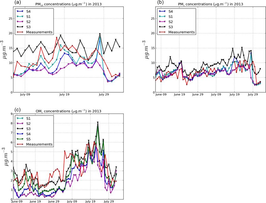
2012 and 2013 summers, and against airborne measurements 2013. The time series of measured and simulated PM10 and
from the ATR-42 flight on 10 July 2014. The criteria of PM1 during the 2013 summer are presented in Fig. C1 of
Boylan and Russell (2006) are used to evaluate the model- Appendix C.
to-measurement comparisons. The performance criterion is PM10 and PM1 are well modeled during both the 2012 and
verified if |MFB| ≤ 60 % and MFE ≤ 75 % (MFB and MFE 2013 summer campaigns, and the performance and goal cri-
stand for the respective mean fractional bias and the mean teria are always met. The measured mean concentration of
fractional error and are defined in Table A1 of Appendix A), PM1 is very similar in 2012 and 2013 (7.6 and 7.0 µg m−3 , re-
while the goal criterion is verified if |MFB| ≤ 30 % and spectively). However, the mean PM10 concentration in 2012
MFE ≤ 50 %. To evaluate the sensitivity of the modeled con- is double that of 2013 (22.4 and 11.5 µg m−3 , respectively),
centrations to input data, the different simulations summa- which is most likely due to the higher occurrence of trans-
rized in Table 1 are compared to the reference simulation S1 ported desert dust in 2012 (Nabat et al., 2015).
by computing the normalized root mean square error (RMSE Although the mean PM1 and PM10 concentrations are well
of the concentration differences between a simulation and S1, modeled in 2013, the mean PM1 concentration is slightly un-
divided by the mean concentration of S1). derestimated during summer 2013 and the mean PM10 con-
centration is slightly underestimated in 2012. The underesti-
4.1 PM10 and PM1 mation of PM10 may be due to difficulties in accurately rep-
resenting the transported dust episodes, which are frequent in
summer in the western Mediterranean (Moulin et al., 1998)
The statistical scores of the simulated PM1 and PM10 are
shown in Table 7 for the summer campaigns of 2012 and
Atmos. Chem. Phys., 18, 9631–9659, 2018 www.atmos-chem-phys.net/18/9631/2018/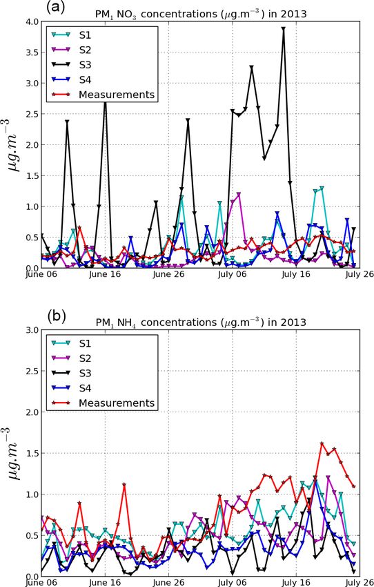
M. Chrit et al.: Aerosol sources in the western Mediterranean during summertime                                                9639

Table 7. Comparisons of simulated PM10 , PM1 and OM1 daily concentrations to observations (concentrations and RMSE are in µg m−3 )
during the summer campaign periods of 2012 (between 9 June and 3 July) and 2013 (between 7 June and 3 August). s stands for simulated
mean and o stands for observed mean. Simulation details are given in Table 1.

                                   PM10 (2012)     PM1 (2012)     OM1 (2012)      PM10 (2013)    PM1 (2013)    OM1 (2013)
         Measured mean o                  22.38           7.57             3.89         11.46           7.02           2.88
              s ± RMSE              16.44 ± 7.55   9.40 ± 2.72     3.39 ± 0.78     9.69 ± 3.17   6.98 ± 1.77    2.56 ± 1.07
              Correlation (%)               76.8          78.9            95.2            70.9          67.5             81
         S1

              MFB                            -30            18            −20             −19            −1            −17
              MFE                             30            27              23              26            20             35
              s ± RMSE                         –             –               –     7.49 ± 4.75   6.42 ± 1.91    1.61 ± 1.62
         S2

              Diff. with S1 (%)                –             –               –            −23            −8            −37
              Norm. RMSE (%)                   –             –               –              33            21             49
              s ± RMSE                         –             –               –    14.94 ± 5.02   9.45 ± 2.95    3.26 ± 1.03
         S3

              Diff. with S1 (%)                –             –               –              54            35             27
              Norm. RMSE (%)                   –             –               –              65            40             29
              s ± RMSE            13.87 ± 10.95    7.66 ± 1.56     2.37 ± 1.64     8.48 ± 4.02   6.86 ± 2.03    1.98 ± 1.29
         S4

              Diff. with S1 (%)            −16            −19             −30             −12            −2            −23
              Norm. RMSE (%)                 23              2              43              17            10             32
              s ± RMSE                         –             –               –              –              –    2.54 ± 1.07
         S5

              Diff. with S1 (%)                –             –               –              –              –            −1
              Norm. RMSE (%)                   –             –               –              –              –              1

and are represented in the Mediterranean simulation by dust          Italy) contributes to a small portion of PM10 (5 % in 2012 and
boundary conditions from the global model MOZART4.                   7 % in 2013). Saharan dust can be transported by air masses
   The comparisons of the different simulations at Ersa in           to the Mediterranean atmosphere via medium-range trans-
Table 7 show that both PM10 and PM1 concentrations are               port and is an important component of PM10 , with respective
strongly influenced by sea-salt emissions (S3, with a normal-        contributions of 34 and 21 % during the summer campaigns
ized RMSE of 65 and 40 %, respectively), especially as the           of 2012 and 2013.
emissions of the two parameters differ by as much as 1400 %             The PM1 mass is dominated by organic matter (41 % in
over the sea in southern France (Sect. 2.1). PM10 and PM1            2012 and 38 % in 2013) and sulfate (30 % in 2012 and 24 %
concentrations are also very sensitive to meteorology (S2,           in 2013). The percentage of sodium (from sea salt) is signif-
with a normalized RMSE of 33 and 21 %, respectively) and             icant in PM10 (4 % in 2012 and 10 % in 2013); however, it is
anthropogenic emissions (S4, with a normalized RMSE of               negligible in the PM1 mass (less than 1 %).
17 and 10 %, respectively).
   Knowing the chemical composition of PM10 and PM1 pro-             4.2    OM1
vides important information to aid with deciphering the dif-
ferent sources of aerosol particles arriving at Ersa, and to         The statistical evaluation of OM1 during the summer cam-
understand the sensitivities presented above. Figure 3 shows         paigns of 2012 and 2013 is available in Table 7. As dis-
the simulated composition of PM10 and PM1 , the percent-             cussed in Chrit et al. (2017), the performance and goal cri-
age contribution of each compound to PM in 2013, and the             teria are both satisfied, due to the addition of highly oxi-
associated variability.                                              dized species (extremely low volatility organic compounds,
   According to simulation, inorganic aerosols account for           organic nitrate and the carboxylic acid MBTCA (3-methyl-
a large part of the PM10 mass: during the summer cam-                1,2,3-butanetricarboxylic acid) as a second generation oxida-
paign periods of 2012 and 2013, the inorganic fraction in            tion product of α-pinene) in the model. Adding these species
PM10 is 31 and 39 %, respectively. Among inorganics, sul-            to the model was also required to correctly model OM prop-
fate, largely originating from anthropogenic sources, occu-          erties (oxidation state and affinity to water). The time se-
pies a large portion of PM10 (18 % in 2012 and 19 % in               ries of measured and simulated OM1 concentrations during
2013). The organic mass (OM) also largely contributes to             the summer 2013 campaign are presented in Fig. C1 of Ap-
PM10 (30 % in 2012 and 33 % in 2013). Black carbon (origi-           pendix C. The comparison of the different simulations at Ersa
nating from traffic and shipping emissions and industrial ac-        in Table 7 shows that OM1 is particularly influenced by me-
tivities in big cities in the south of France and the north of       teorology (S2 with a normalized RMSE of 49 %), because

www.atmos-chem-phys.net/18/9631/2018/                                                 Atmos. Chem. Phys., 18, 9631–9659, 2018
9640                                      M. Chrit et al.: Aerosol sources in the western Mediterranean during summertime

Figure 3. PM10 (a) and PM1 (b) average relative simulated composition during the summer 2013 campaign period.

Table 8. Comparisons of simulated PM1 inorganic daily concentrations to observations (concentrations are in µg m−3 ) using S1 and S4
during the 2012 summer.

                             Inorganics                            Nitrate       Sulfate   Ammonium
                             Measured mean o                         0.41          2.06           1.39
                                  Simulated mean s ± RMSE      0.51 ± 0.28   2.53 ± 1.13   0.68 ± 0.85
                                  Correlation (%)                     20.1          71.4          47.8
                             S1

                                  MFB                                   15            31           -72
                                  MFE                                   50            39            72
                                  Simulated mean s ± RMSE      0.53 ± 0.36   1.71 ± 1.28   0.50 ± 1.04
                             S4

                                  Diff. with S1 (%)                  +4 %         −32 %         −26 %
                                  Norm. RMSE (%)                        45            46            32

meteorology influences biogenic emissions; however, OM1             2013 summer campaign. The time series of measured and
is also affected by inorganic sea-salt emissions (S3 with a         simulated inorganic concentrations during the 2013 summer
normalized RMSE of 29 %), which provide mass onto which             campaign are presented in Figs. C2 and C3 of Appendix C.
hydrophilic SOA (secondary organic aerosol) can condense               Inorganic concentrations of PM1 aerosol were measured in
(especially sulfate). Furthermore, anthropogenic emissions          2012, and both PM1 and PM10 were measured in 2013. Some
(S4 with a normalized RMSE of 32 %), which affect the for-          of the inorganic gaseous precursors (SO2 , HNO3 and HCl)
mation of oxidants through photochemistry and emit anthro-          were also measured for just a few days in 2013 (between
pogenic precursors also impact OM1 . The sensitivity to an-         21 and 26 July 2013).
thropogenic I/S-VOC emissions is low (S5, with a normal-               For the 2012 reference simulation (S1), the PM1 , sulfate
ized RMSE of only 1 %).                                             and nitrate concentrations satisfy both the performance and
                                                                    goal criteria. However, ammonium concentrations are under-
4.3     Inorganic species                                           estimated, despite the performance criterion being satisfied
                                                                    in terms of the MFE. This underestimation of ammonium
4.3.1    Ground-based evaluation                                    increases if the EMEP emission inventory with lower ship
                                                                    emissions over the Mediterranean Sea is used, suggesting
The statistical scores of the simulated inorganic concentra-        that ammonium nitrate formation is strongly dependent on
tions are shown in Table 8 for PM1 concentrations during            ship NOx emissions (because they lead to the formation of
the summer 2012 campaign and in Tables 9 and 10 for PM10            the gaseous precursors of ammonium nitrate).
and PM1 inorganic concentrations, respectively, during the

Atmos. Chem. Phys., 18, 9631–9659, 2018                                               www.atmos-chem-phys.net/18/9631/2018/
M. Chrit et al.: Aerosol sources in the western Mediterranean during summertime 9641
Table 9. Comparisons of simulated PM10 inorganic daily concentrations to observations (concentrations are in µg m−3 ) using S1, S2, S3 and
S4 during the 2013 summer.
Inorganics Nitrate Sulfate Ammonium Chloride Sodium
Measured mean o 0.42 1.52 0.76 0.18 0.53
Simulated mean s ± RMSE 0.33 ± 0.42 2.05 ± 0.84 0.58 ± 0.39 0.12 ± 0.45 0.70 ± 0.54
Correlation (%) 5.7 69.7 47.6 −11.4 55.5
S1
MFB −43 32 −20 −67 30
MFE 86 40 43 105 70
Simulated mean s ± RMSE 0.19 ± 0.46 2.10 ± 0.82 0.49 ± 0.44 0.13 ± 0.44 0.77 ± 0.57
S2
Diff. with S1 (%) −42 % +2 % −16 % +8 % +10 %
Norm. RMSE (%) 130 22 52 100 43
Simulated mean s ± RMSE 0.88 ± 1.27 2.14 ± 0.97 0.31 ± 0.60 0.59 ± 1.14 1.77 ± 2.34
S3
Diff with S1 (%) +167% +4 % −47 % +392 % +153 %
Norm. RMSE (%) 376 22 62 933 291
Simulated mean s ± RMSE 0.24 ± 0.41 1.33 ± 0.67 0.34 ± 0.56 0.27 ± 0.64 0.98 ± 0.77
S4
Diff. with S1 (%) −27 % −35 % −41 % +125 % +40 %
Norm. RMSE (%) 66 44 48 267 50
Table 10. Comparisons of simulated PM1 inorganic daily concentrations to observations (concentrations are in µg m−3 ) using S1, S2, S3
and S4 during the 2013 summer.
Inorganics Nitrate Sulfate Ammonium
Measured mean o 0.30 1.47 0.65
Simulated mean s ± RMSE 0.32 ± 0.31 1.86 ± 0.94 0.58 ± 0.38
Correlation (%) 22.9 28.9 32
S1
MFB −24 27 −6
MFE 77 55 55
Simulated mean s ± RMSE 0.18 ± 0.28 1.72 ± 0.66 0.50 ± 0.52
S2
Diff. with S1 (%) −44 % −8 % −14 %
Norm. RMSE (%) 134 19 44
Simulated mean s ± RMSE 0.87 ± 1.20 1.89 ± 0.81 0.31 ± 0.50
S3
Diff. with S1 (%) +172 % +2 % −47 %
Norm. RMSE (%) 384 29 62
Simulated mean s ± RMSE 0.23 ± 0.25 1.08 ± 0.71 0.34 ± 0.48
S4
Diff. with S1 (%) −28 % −42 % −41 %
Norm. RMSE (%) 69 34 47
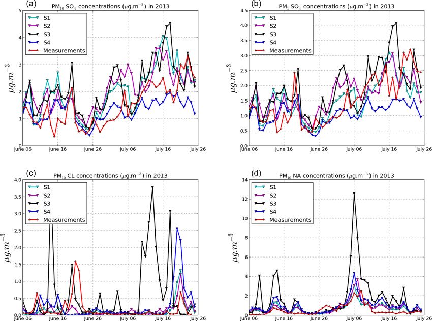
For the 2013 reference simulation (S1), PM10 , sulfate and as high as about 5 K in daily points) and difficulties in rep-
ammonium satisfy the both performance and goal criteria, resenting the partitioning between gas and particle phases.
while sodium satisfies only the performance criterion. The For chloride, as shown in Fig. C2 in Appendix C, although
mean concentrations of modeled chloride and nitrate are both the mean concentration is underestimated, the peaks are
underestimated. This underestimation is probably due to un- overestimated. For example, between 21 and 26 July 2013,
certainties in the measurements. In fact, nitrate and chlo- the particle-phase chloride concentration is 0.34 µg m−3 in
ride are difficult to measure, as there can be negative arti- the simulation, but only 0.05 µg m−3 in the measurements.
facts (volatilization of the aerosol phase during sampling) The total chloride (gas + particle phase) is well modeled
or positive artefacts (condensation of gaseous phase onto the (1.2 µg m−3 in the measurements and 1 µg m−3 simulated),
particles or filters during sampling), depending on the sam- but the gas / particle ratio is much higher in the measure-
pling conditions. Moreover, this underestimation may be also ments (18.4) than in the model (2.4). For nitrate, the to-
due to uncertainties in the modeled temperature (with bias tal nitrate (gas + particle phase) is overestimated between
www.atmos-chem-phys.net/18/9631/2018/ Atmos. Chem. Phys., 18, 9631–9659, 20189642 M. Chrit et al.: Aerosol sources in the western Mediterranean during summertime 21 and 26 July 2013 (2.7 µg m−3 in the measurements and 6.6 µg m−3 simulated), and most of it is in the gas phase (only 0.4 µg m−3 in the particle phase in the measurements and 0.2 simulated). Contrary to chloride, the gas / particle ratio for nitrate is much higher in the model (28.2) than in the measurements (5.4). The reason for the difficulties in representing the gas / particle ratios of chloride is that the measured PILS chloride concentrations only include non- refractory chloride. The reason for the difference in the ni- trate ratio is likely related to the internal mixing hypothesis and the bulk-equilibrium assumption in the modeling of con- densation/evaporation. This is investigated in the following section, during the comparison to airborne measurements. For the 2013 reference simulation (S1), PM1 , PM10 , sul- Figure 4. Measurements are averaged at four model levels from fate and ammonium satisfy the performance criterion, which airborne observations below 800 m a.g.l along the flight path shown is also almost satisfied for nitrate. The measured and simu- in Fig. 1 on 10 July 2014. The concentrations of the S1 simulations lated PM1 and PM10 concentrations are relatively similar for (standard and with options; see text for details) are also averaged sulfate and ammonium, suggesting that most of the mass is in time along the flight path. Results from S1 and from S1-without- in PM1 . SO4 in SSE (sea-salt emissions) are quite similar. The comparisons of the different simulations at Ersa in Tables 9 and 10 show that inorganics in PM10 and PM1 have similar sensitivities, because of the bulk equilibrium as- 4.4 Airborne evaluation sumption made in the modeling of condensation/evaporation. Sulfate is more sensitive to anthropogenic (ship) emissions The measurement flight considered in this study (with a normalized RMSE of 44 % in PM10 ) than meteorol- (10 July 2014, 10:21–14:09 UTC) was conducted by ogy (with a normalized RMSE of 22 %) and sea-salt emis- the French ATR-42 aircraft deployed by SAFIRE in the sions (with a normalized RMSE of 22 %). Nitrate, chloride south of France above the Mediterranean Sea. The purpose and sodium, and ammonium to a lower extent, are highly of the flight was to study aerosol formation, evolution and sensitive to sea-salt emissions with normalized RMSEs be- properties in marine conditions, under the mistral regime tween 62 and 933 % (the Jaegle et al. (2011) parameterization (north/northwest winds coming from the Rhône Valley char- has a lower dependance on wind speed than the Monahan et acterized by high wind speeds). Altitudes and a horizontal al. (1986) parameterization). They are also strongly affected projection of the trajectory of the aircraft during the flight by meteorology (with normalized RMSEs between 43 and are presented in Fig. 1. The aircraft flew at low altitudes 130 %), because meteorology affects natural emissions (sea (under 800 m a.s.l.) over the Mediterranean Sea for about salt and biogenic), as discussed in Sect. 5. By influencing 2 h, allowing us to evaluate the modeling of sea-salt aerosols. biogenic emissions, meteorology affects the formation of or- As shown in Fig. 1, the planetary boundary layer height, as ganics (Sartelet et al., 2012), as they are mostly of biogenic modeled by ECMWF meteorological fields, exhibit strong origin in summer (Chrit et al., 2017). The influence of mete- spatial variations. orology on biogenic emissions also affects the formation of For the comparisons of inorganic concentrations to air- inorganics, due to the modification of oxidant concentrations borne measurements, the reference simulation S1 is run a few (Aksoyoglu et al., 2017) and the temperature bias that can be days during the summer 2014. The simulated concentrations as high as 5 K, in addition to the formation of organic nitrate are extracted along the flight path from the corresponding (Ng et al., 2017). Inorganic concentrations are also strongly grid cells and layers. For the model-to-measurement com- affected by anthropogenic emissions (with normalized RM- parisons, only the cells were the plane was flying above the SEs between 44 and 267 %), owing to the fact that anthro- sea, at low altitudes (below 800 m a.s.l.) with a spatially uni- pogenic emissions affect the NOx emissions; hence, the oxi- form boundary layer (above 1200 m) are considered. The dants and the formation of both organic and inorganic nitrate transects where model-to-measurement comparisons are per- is also impacted. Because nitrate, ammonium and chloride formed are indicated by purple crosses/lines in Fig. 1. The partition between the gas and particle phases, their uncertain- meteorological fields during this flight are compared with ties are linked and they are strongly affected by assumptions measured data in Appendix F. The mistral regime is simu- in the modeling of condensation/evaporation, as detailed in lated with wind directions that are well modeled, although the Sect. 4.4. wind speeds are underestimated. Atmos. Chem. Phys., 18, 9631–9659, 2018 www.atmos-chem-phys.net/18/9631/2018/
M. Chrit et al.: Aerosol sources in the western Mediterranean during summertime                                                   9643

Figure 5. Vertical profile averaged at four model levels of NO3 (a) and NH4 (b). Measurements are averaged at the same four model levels
from airborne observations below 800 m a.g.l along the flight shown in Fig. 1 on 10 July 2014 (around noon).

4.4.1   Sulfate                                                       4.4.2   Ammonium and nitrate

Figure 4 shows the comparison of sulfate to the airborne              Figure 5 shows the comparison of nitrate and ammonium
measurements using different model configurations. Sulfate            concentrations in PM1 . The simulated means of ammonium
is the inorganic compound with the highest PM1 concentra-             and nitrate are about 0.32 and 0.14 µg m−3 , respectively. In
tions (about 0.54 µg m−3 ).                                           the reference simulation ,S1, ammonium and nitrate are un-
   As shown in Fig. 4, the PM1 sulfate concentration is over-         derestimated compared to the measurements.
estimated in the simulation with a mean concentration of                 Figure 5 shows the comparison of nitrate and ammo-
about 0.55 µg m−3 compared to 0.47 µg m−3 in the measure-             nium concentrations in PM1 to the airborne measurements
ments. To understand the reasons for this overestimation, dif-        using different model configurations. Because ammonium,
ferent sensitivity simulations are performed. The first sensi-        nitrate and chloride are semi-volatile inorganic species,
tivity simulation (referred to as “S1-without-SO4 in SSE”,            their concentrations may depend on the assumptions made
where SSE stands for sea-salt emissions) differs from the S1          in the modeling of condensation/evaporation. In the ref-
simulation due to the fact that sulfate is only emitted from an-      erence simulation, bulk thermodynamic equilibrium is as-
thropogenic sources and marine sulfate is not taken into ac-          sumed between the gas and particle phases for all inorganic
count. The second sensitivity simulation (referred to as “S1-         species. In the first sensitivity simulation (referred to as “S1-
H2 SO4 -0 %”) differs from S1 in that SOx emissions are split         Dynamic”), the condensation/evaporation is computed dy-
into 100 % of SO2 and 0 % of H2 SO4 , instead of 98 % of SO2          namically rather than assuming thermodynamic equilibrium.
and 2 % of H2 SO4 (as in S1). The measurement-to-model                In the second sensitivity simulation (referred to as “S1-IA-
comparison of the vertical profile of the PM1 sulfate concen-         externally-mixed”), sea-salt (chloride and sodium) emissions
trations using the three simulations is shown in Fig. 4. The in-      are assumed not to be mixed with the other aerosols. In S1-
fluence of marine sulfate is negligible: the simulated means          IA-externally-mixed, bulk equilibrium is assumed for ammo-
using S1 with and without the emissions of marine sulfate             nium, nitrate and sulfate, while chloride and sodium do not
are nearly equal (≈ 0.55 µg m−3 ) indicating that the PM1             interact with the other inorganic species.
sulfate concentration is almost totally from anthropogenic               Under the thermodynamic equilibrium approach (S1), ni-
sources. A comparison of PM10 sulfate concentrations for              trate is underestimated (the measured and simulated means
the two simulations show that this is also the case for PM10 .        are 0.10 and 0.05 µg m−3 , respectively). This is likely be-
This is indicative of the overestimation of sulfate or sulfuric       cause the sulfate is overestimated, as detailed in Sect. 4.4.1,
acid emissions, or of issues with the treatment of emissions          but also because the assumption of thermodynamic equilib-
from ship stacks in the model . However, PM1 sulfate con-             rium between the gas and particle phases is not verified. Ni-
centrations are strongly influenced by anthropogenic emis-            trate concentrations are closer to measurements if conden-
sions. For example, PM1 sulfate concentrations are lower if           sation/evaporation is computed dynamically, especially be-
the fraction of H2 SO4 in the SOx emissions is lower than             tween 400 and 600 m in altitude, where the mean concentra-
in the reference simulation (the simulated mean concentra-            tions are 0.07 µg m−3 in the measurements (0.02 µg m−3 with
tions with and without H2 SO4 in SOx emissions are 0.55               S1 and 0.07 µg m−3 with S1-Dynamic). If sea-salt aerosols
and 0.52 µg m−3 , respectively), because of the rapid conden-         are externally mixed, than nitrate is even more underesti-
sation of H2 SO4 (which has a saturation vapor pressure of            mated than in S1. This is because nitrate tends to replace
almost zero) onto particles.                                          chloride in sea salt if thermodynamic considerations are
                                                                      taken into account.

www.atmos-chem-phys.net/18/9631/2018/                                                   Atmos. Chem. Phys., 18, 9631–9659, 2018
You can also read