Measurements of CFC-11, CFC-12, and HCFC-22 total columns in the atmosphere at the St. Petersburg site in 2009-2019
←
→
Page content transcription
If your browser does not render page correctly, please read the page content below
Atmos. Meas. Tech., 14, 5349–5368, 2021
https://doi.org/10.5194/amt-14-5349-2021
© Author(s) 2021. This work is distributed under
the Creative Commons Attribution 4.0 License.

Measurements of CFC-11, CFC-12, and HCFC-22 total columns in
the atmosphere at the St. Petersburg site in 2009–2019
Alexander Polyakov, Anatoly Poberovsky, Maria Makarova, Yana Virolainen, Yuri Timofeyev, and
Anastasiia Nikulina
Department of Atmospheric Physics, St. Petersburg State University, 7–9 Universitetskaya Emb.,
St. Petersburg 199034, Russia

Correspondence: Alexander Polyakov (a.v.polyakov@spbu.ru)

Received: 28 August 2020 – Discussion started: 17 October 2020
Revised: 1 June 2021 – Accepted: 5 July 2021 – Published: 4 August 2021

Abstract. Monitoring atmospheric anthropogenic halocar-             In general, the comparison of Xgas with the independent
bons plays an important role in tracking their atmospheric       data showed a good agreement of their means within the sys-
concentrations in accordance with international agreements       tematic errors of the measurements considered. The trends
on emissions of ozone-depleting substances and, thus, in es-     observed over the St. Petersburg site demonstrate the smaller
timating the ozone layer recovery.                               decrease rates for XCFC-11 and XCFC-12 than that of the inde-
   Within the Network for the Detection of Atmospheric           pendent data and the same increase rate for XHCFC-22 . As a
Composition Change (NDACC), regular Fourier transform            whole, Xgas, SVMR, and WXgas showed qualitatively sim-
infrared (FTIR) measurements can provide information on          ilar seasonal variations, while the GVMR variability is sig-
the abundancies of halocarbons on a global scale. We im-         nificantly less, and only the WXHCFC-22 variations are essen-
proved retrieval strategies for deriving the CFC-11 (CCl3 F),    tially smaller than that of XHCFC-22 and SVMRHCFC-22 .
CFC-12 (CCl2 F2 ), and HCFC-22 (CHClF2 ) atmospheric
columns from IR solar radiation spectra measured by the
Bruker IFS125HR spectrometer at the St. Petersburg site
(Russia). We used the Tikhonov–Phillips regularization ap-       1   Introduction
proach for solving the inverse problem with optimized
values of regularization parameters. We tested the strate-       Since the middle of the 20th century, anthropogenic trace
gies developed by comparison of the FTIR measurements            gases, the molecules of which contain halogens, due to their
with independent data. The analysis of the time series of        specific physical and chemical properties, have been actively
column-averaged dry air mole fractions (Xgas) measured in        used in the climatic and refrigeration industry, as well as in
2009–2019 gives mean values of 225 pptv (parts per tril-         various propellants. Molina and Rowland (1974) have shown
lion by volume; CFC-11), 493 pptv (CFC-12), and 238 pptv         that these gases play an important role in the destruction of
(HCFC-22). Trend values total −0.40 % yr−1 (CFC-11),             stratospheric ozone. In particular, the photolysis of CCl3 F
−0.49 % yr−1 (CFC-12), and 2.12 % yr−1 (HCFC-22).                (trichlorofluoromethane; CFC-11) and CCl2 F2 (dichlorodi-
   We compared the means, trends, and seasonal variability       fluoromethane; CFC-12) in the stratosphere leads to the ap-
in XCFC-11 , XCFC-12 , and XHCFC-22 to that of (1) near-ground   pearance of active chlorine, which is involved in ozone deple-
volume mixing ratios (VMRs), measured at the observational       tion reactions. The WMO (2018, Appendix A) estimates the
site Mace Head, Ireland (GVMR), (2) the mean in the 8–           ozone depletion potential (ODP) of CFC-12 as being 0.73–
12 km layer VMRs, measured by ACE-FTS and averaged               0.81 (the ODP of CFC-11, chosen as a reference, equals 1).
over 55–65◦ N latitudes (SVMR), and (3) Xgas values of the       Although the major content of these gases is concentrated in
Whole Atmosphere Community Climate Model (WACCM)                 the troposphere, in the equatorial region, the global circula-
for the St. Petersburg site (WXgas).                             tion moves them out into the lower and middle stratosphere
                                                                 and transports them to high-latitude regions. In the strato-

Published by Copernicus Publications on behalf of the European Geosciences Union.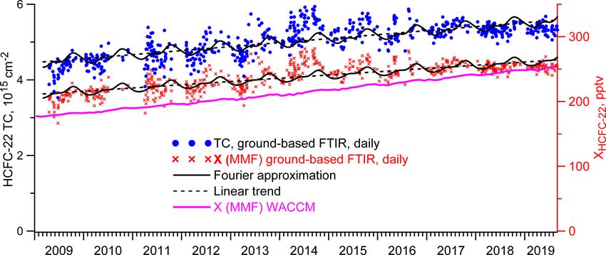
5350                           A. Polyakov et al.: Measurements of CFC-11, CFC-12, and HCFC-22 atmospheric content

sphere, chlorofluorocarbons (CFCs) are photochemically de-         decreasing trends in CFC-11 (−0.53 % yr−1 ) and CFC-12
composed to chlorinated free radicals (Cl and ClO) that are        (−0.61 % yr−1 ) abundancies and a slowing rate of increase
deactivated into chlorine reservoirs of HCl, ClONO2 , and          in HCFC-22 abundancies (1.8 % yr−1 ). ACE-FTS estimates
HOCl (WMO, 1985, Chapter 3). In polar regions, heteroge-           are made for latitudes between 60◦ S and 60◦ N and for alti-
neous reactions on the surfaces of polar stratospheric clouds      tudes between 5.5 and 10.5 km. Nevertheless, with its accu-
and cold sulfate aerosols convert inert reservoir molecules        mulation in the troposphere, CFC-11 still provides a quarter
into active forms that photolyze, producing free radicals, and     of all chlorine reaching the stratosphere. The time needed for
cause the chemical ozone depletion in spring through cat-          recovery of the ozone layer depends, among other factors, on
alytic cycles resulting up to the appearance of ozone holes        the sustainability of the reduction in the atmospheric concen-
(Solomon et al., 2014).                                            trations of CFC-11, CFC-12, and other halocarbons.
   As the result of the Montreal Protocol and its amend-              Based on the 2015–2017 data, Montzka et al. (2018)
ments and adjustments that restricted the production of CFCs       showed that the rate of change in the CFC-11 atmo-
(see WMO, 2018), the industry moved away from CFCs                 spheric concentrations decreased by approximately half to
to less ozone-depleting hydrochlorofluorocarbons (HCFCs),          −0.4 % yr−1 , assuming that this slowdown is caused by
especially CHClF2 (chlorodifluoromethane; HCFC-22). Al-            the emergence of new, unregistered sources. This find-
though the ODP of HCFC-22 is much lower than that of               ing enhances the importance of the CFC-11 monitor-
CFCs, it is an ozone-depleting substance too. Ozone deple-         ing. The maximum of the CFC-12 atmospheric concen-
tion by HCFC-22 is primarily associated with the heating of        trations was observed in the early 2000s; since then, its
the stratosphere, and its ODP, although small, totals 0.024–       steady decrease has been detected with an average rate of
0.34.                                                              0.4 % yr−1 to 0.5 % yr−1 (Advanced Global Atmospheric
   CFC-11 and CFC-12, like HCFC-22, also absorb infrared           Gases Experiment (AGAGE) network; http://agage.mit.edu/
radiation; therefore, they are all greenhouse gases. The global    data/agage-data, last access: 3 August 2020). As HCFCs are
warming potential (GWP) represents the integrated radiative        “transitional substances” for the replacement of CFCs, their
forcing (RF) for a conditional time horizon (20, 100, and          production has increased rapidly in developed countries in
500 years) caused by emissions of a unit mass of a gas rel-        the 1990s and peaked in the mid-1990s. Under the Montreal
ative to the same RF value of CO2 that is chosen as a ref-         Amendment (1997), all countries must gradually phase down
erence for estimating the GWP of other gases. According to         HCFCs. In September 2007, it was decided to accelerate the
WMO (2018, Appendix A), the GWP for 100 years is 5160              phasing out of HCFCs. Developed countries were reducing
for CFC-11, 10 300 for CFC-12, and 1780 for HCFC-22. One           their consumption of HCFCs and completely phased them
of the reasons for the high GWP values of these gases is their     out by 2020. Developing countries agreed to start their phase-
long lifetimes, i.e., 52, 102, and 11.9 years, respectively. Due   out process in 2013 and are now following a stepwise reduc-
to their long lifetimes, these gases are also good indicators      tion until the complete phase out of HCFCs by 2030.
for studying the transport and mixing processes in the upper          On a global scale, two data sources are mainly used to
troposphere and the lower stratosphere (e.g., Hoffmann and         study the trends and seasonal variations in the target gases,
Riese, 2004).                                                      i.e., local measurements of near-ground concentrations (e.g.,
   After Molina and Rowland (1974) reported that the CFCs          the AGAGE networks, Dunse et al., 2005, NOAA’s Halocar-
accumulating in the Earth’s atmosphere led to an increased         bons & other Atmospheric Trace Species (HATS) and Chlo-
rate of ozone depletion, the attention of both scientists and      rofluorocarbon Alternatives Monitoring Project (CAMP),
policymakers to the ozone hole problem increased. Nowa-            Montzka et al., 1993), and satellite limb measurements by the
days, monitoring of ozone and other stratospheric gases, as        Improved Limb Atmospheric Spectrometer (ILAS), ACE-
well as ozone-depleting substances, including CFCs, is cru-        FTS, and Michelson Interferometer for Passive Atmospheric
cial for testing the theories of the ozone hole formation mech-    Sounding (MIPAS; Hoffmann et al., 2008; Mahieu et al.,
anism (Cracknell and Varotsos, 2009).                              2008; Eckert et al., 2016; Kellmann et al., 2012; Boone
   The Montreal Protocol from 1987, which came into force          et al., 2020). In contrast to satellite and in situ measure-
in 1989, limited the production and consumption of CFCs.           ments near ground, ground-based Fourier transform infrared
Later on, in 1992, in Copenhagen, and in 1995, in Vienna,          (FTIR) measurements of solar radiation are sensitive to
the phasing out of CFCs was started by the end of 1995             changes in total columns (TCs) of atmospheric gases. The
in developed countries and by the end of 2010 in develop-          FTIR method complements the information obtained by the
ing countries. Therefore, the atmospheric burden of CFC-11         first two methods, although it does not allow detailed infor-
and CFC-12 was declining at an average rate of 0.7 % yr−1 –        mation on the vertical gas distribution to be retrieved.
1.2 % yr−1 and 0.4 % yr−1 –0.5 % yr−1 , respectively (Brown           The first FTIR measurements of atmospheric HCFC-22
et al., 2011). ACE-FTS (Atmospheric Chemistry Experi-              were performed from the balloon in early 1980s (Gold-
ment and Fourier transform spectrometer) satellite measure-        man et al., 1981). Later, with the appearance of high-
ments in the last 16 years (Bernath et al., 2020a) have illus-     resolution instruments, halocarbons started to be derived
trated the success of the Montreal Protocol by demonstrating       with ground-based FTIR spectrometers. In the last few

Atmos. Meas. Tech., 14, 5349–5368, 2021                                             https://doi.org/10.5194/amt-14-5349-2021
A. Polyakov et al.: Measurements of CFC-11, CFC-12, and HCFC-22 atmospheric content 5351
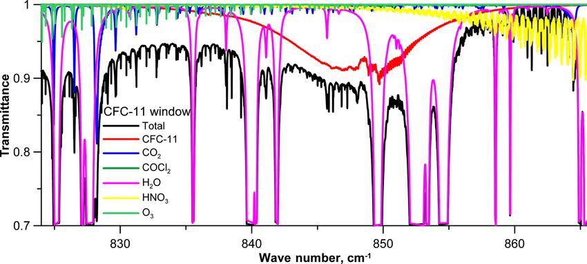
decades, TCs of halocarbons are more actively measured as being 96 % and 95 %, respectively. Second, there is the
by ground-based FTIR methods (e.g., Notholt, 1994; Rins- absorption of interfering gases in the spectral range consid-
land et al., 2005, 2010; Zander et al., 2005; Mahieu et al., ered. Thus, the CFC-11 absorption band overlaps with sev-
2010, 2013, 2017; Zhou et al., 2016; Prignon et al., 2019). eral strong water vapor absorption lines and the HNO3 ab-
Time series of CFC-11, CFC-12, and HCFC-22 TCs above sorption band, and each of the CFC-12 and HCFC-22 ab-
the Jungfraujoch station, Switzerland, are presented in World sorption bands overlap a wing of the water vapor absorption
Meteorological Organization (WMO) reports on the scien- line (see Appendix A). Finally, the CFC-12 and, to a larger
tific assessment of ozone depletion (e.g., WMO, 2018). extent, the CFC-11 bands have a smoothed spectral depen-
Within the Network for the Detection of Atmospheric dency of absorption that requires the use of wide microwin-
Composition Change (NDACC; http://www.ndaccdemo. dows for retrieving their abundancies, i.e., 2 cm−1 for CFC-
org/, last access: 28 July 2021), regular FTIR measurements 12 and not smaller than 30 cm−1 for CFC-11. These factors
provide information on TCs of a number of atmospheric trace cause difficulties in halocarbon retrieval from FTIR spectra
gases, including halocarbons, with a large spatial coverage measurements.
(at 19 out of 77 network stations located at latitudes between Later, the retrieval techniques for estimating CFC-11,
78◦ S and 80◦ N). Mahieu et al. (2017) reported on the re- CFC-12, and HCFC-22 TCs by the FTIR method at
sults of R-142b measurements, along with the comparison the St. Petersburg site were refined and improved. These
with independent data and the trend estimates. Zhou et al. techniques were described in detail by Polyakov et al.
(2016) showed the results of CFC-11, CFC-12, and HCFC- (2019a, b, 2020b). In the current study, we present the main
22 measurements at two NDACC sites on Réunion island for features of the techniques developed and analyzed using
the period of 2004–2016, including the trend estimates and the Tikhonov–Phillips (T−Ph) approach. The time series of
the comparison with the satellite data. Prignon et al. (2019) CFC-11, CFC-12, and HCFC-22 TCs were extended until the
proposed a technique for estimating two partial columns and fall of 2019. The time series of the TCs were analyzed and
TCs of HCFC-22 at the Jungfraujoch mountain station and a compared to independent measurements and numerical mod-
corresponding time series of HCFC-22 TCs for 1988–2017, eling data.
along with a trend analysis for various time periods.
The archive of ground-based spectroscopic measurements
of IR solar radiation, performed at the NDACC site of St. Pe- 2 Technique for inverting the spectroscopic
tersburg (Timofeyev et al., 2016; Virolainen et al., 2017) measurements
since 2009, has been used to derive TCs of CFC-11, CFC-
2.1 Spectroscopic measurements
12, and HCFC-22. First, in Russia, estimates of CFC-11 TCs
using the FTIR method and the original retrieval technique The main features of the ground-based station, observational
were given by Yagovkina et al. (2011). Polyakov et al. (2018) system, and the technique for measuring the solar spectra
presented the preliminary results of CFC-11, CFC-12, and used in this study were described in detail by Timofeyev et
HCFC-22 TCs retrieval for the period of 2009–2016, using al. (2016).
the SFIT4 software (version 0.9.4.4) described by Hase et al. The St. Petersburg site is located in Peterhof, 30 km
(2004). It should be noted that the SFIT4 software is a ver- west of the city of St. Petersburg. The latitude of the site
satile tool, and it is necessary to customize it for a specific (59.88◦ N) predetermines winter measurements with a low
task through the selection and tuning of numerous parame- solar elevation; in December–January, the maximal solar
ters. Polyakov et al. (2018) selected these parameters, based elevation does not usually exceed 20◦ , and spectroscopic
on the studies at other NDACC sites (Mahieu et al., 2010; measurements are performed up to a solar elevation of 5◦ .
Zhou et al., 2016), and the general recommendations of the Due to peculiarities of the local weather, measurements are
IR working group (IRWG) of the NDACC network. How- mainly (76 %) carried out in the spring and summer sea-
ever, these first results raised a several problems; in particu- sons. The spectra analyzed are obtained without any addi-
lar, there was an unreasonably large scatter of the TC values tional apodization of the interferograms, and their spectral
and significant seasonal variations. A later study showed that resolution is 0.005 cm−1 . The observational system is based
the scatter and seasonal variability observed were not due to on a Bruker IFS125HR Fourier spectrometer, but some of
objective reasons but due to peculiarities in the processing the equipment is nonstandard. Before February 2016, a non-
retrieval technique. standard (for the IRWG-NDACC sites) spectral filter (here-
The information content of the FTIR spectra, with respect inafter F3) was used for measurements in a spectral region
to target gases abundancies, is not large, due to several rea- with the absorption bands of the target gases. Since this filter
sons. First, the absorption of CFC-11 and HCFC-22 is not was plane-parallel, a parasitic interference arose in it, lead-
strong. Even for a solar elevation of about 15◦ , the trans- ing to the appearance of an effect of the optical resonance
mission of solar radiation caused by CFC-11 absorption is Blumenstock et al. (“channeling”; see 2020). In addition, a
greater than 90 %, and for HCFC-22, it is close to 75 %. For homemade solar tracking system is used.
a solar elevation of about 50◦ , these values are estimated
https://doi.org/10.5194/amt-14-5349-2021 Atmos. Meas. Tech., 14, 5349–5368, 2021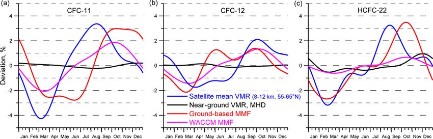
5352                           A. Polyakov et al.: Measurements of CFC-11, CFC-12, and HCFC-22 atmospheric content

   The period of channeling is caused by the material and          (2019a, b, 2020b) used the stability of retrieved total columns
the thickness of the filter, and in the spectral region (800–      in terms of the minimal root mean squared (RMS) standard
900 cm−1 ), it is close to 1.1 cm−1 , while the channeling am-     deviation (SD) of the TCs for all days of measurements as
plitude varies from zero to a few percent, depending ran-          the main criterion in choosing the retrieval parameters. An-
domly on the filter positioning. To analyze the presence and       other important retrieval parameter is the number of degrees
the channeling amplitude, we performed the Fourier analysis        of freedom for signal (DFS) (Rodgers, 2000, p. 19) for tar-
in the most transparent spectral range (892–905 cm−1 ) for         get gases. As a criterion for optimization, the SD of the
harmonic components, with interval periods of 1–1.25 cm−1 .        DFS is minimized. Estimates of total systematic and random
The channeling amplitude was calculated relative to the            measurement errors are also considered. Finally, the spectral
mean signal value in this spectral range.                          residuals (differences between spectra measured and calcu-
   The SFIT4 software supports the accounting for channel-         lated with the retrieved atmospheric state) are analyzed. To
ing, and its compensation is in a spectrum. Before September       estimate the residuals in the SFIT4 software, spectra are nor-
2009, some of the spectra measured had significant values of       malized to the unit, and RMS difference is calculated and
the channeling amplitude. We excluded spectra with a chan-         denoted as χ 2 .
neling amplitude that exceeds 2 % from further processing,             It should be noted that, without additional analysis, the
assuming that such a distortion of the spectra is too great. Af-   listed criteria do not unambiguously determine the optimal
terwards, the filter was installed so as to minimize channel-      retrieval technique. Thus, for example, by adding an un-
ing. In addition, we analyzed the autocorrelation coefficient      known parameter, such as channeling, to the spectra analysis,
of a dark noise in the range of 660–680 cm−1 (except for a         we increase the measurements errors; however, if we remove
slope) and excluded the spectra with an averaged autocor-          it, and residuals become larger, it will indicate that the pa-
relation coefficient greater than 0.1. A large autocorrelation     rameters used are inadequate for real measurements, i.e., the
coefficient of the dark noise indicates the presence of exter-     actual presence of channeling in the spectra. Table 1 high-
nal influences on a measurement process. Moreover, we ex-          lights the main parameters optimized in previous studies.
cluded the spectra that were measured when a haze or clouds            While processing the measured spectra, spectroscopic pa-
were observed in any part of the sky from further processing,      rameters supplied as a part of the SFIT4 software are used.
since the use of these spectra also noticeably increases the       Target gases and COCl2 absorption is calculated based
scatter of the results.                                            on pseudo-lines (see https://mark4sun.jpl.nasa.gov/pseudo.
   As a result of the filtering described, 2901 of 3523 (i.e.,     html, last access: 3 July 2019); other interfering gases ab-
82 %) spectra measured before February 2016 were selected          sorption is calculated based on spectroscopic information
for further processing. In February 2016, the F3 filter was re-    from HITRAN (high-resolution transmission molecular ab-
placed by the standard IRWG NDACC filter, f6, which elimi-         sorption database). The a priori information on the physical
nates the channeling through its wedge-shaped design. Thus,        state of the atmosphere is taken from the NCEP CPC (Na-
the quality of the measurements was improved, and 1903 of          tional Centers for Environmental Prediction Climate Predic-
1958 spectra were selected, giving a sum of 4804 spectra for       tion Center; ftp://ftp.cpc.ncep.noaa.gov/ndacc/ncep/, last ac-
the 2009–2019 period.                                              cess: 1 May 2021); water vapor profiles used in the retrieval
                                                                   are independently derived from the FTIR measurements as
2.2    Main parameters of the retrieval technique                  per the technique described by Virolainen et al. (2017). The
                                                                   a priori profiles of other interfering gases are taken from the
In previous studies, Polyakov et al. (2019a, b, 2020b) deter-      Whole Atmosphere Community Climate Model (WACCM
mined a number of parameters of the retrieval strategy us-         Park et al., 2013). As a first guess for target gases, the
ing the SFIT4 code for deriving the TCs of the target gases        mean profiles of the WACCM data set for the 2009–2019
from the FTIR measurements at the St. Petersburg site, i.e.,       period are used. A wide spectral window for CFC-11 re-
boundaries of microwindows, mean (a priori) of the mea-            trieval (30 cm−1 ; see Table 1) is unusual for deriving the in-
sured gases, the magnitude of and variability in the zero level,   formation on the gas content from high-resolution IR spec-
periods for taking into account (or excluding) channeling,         tra and requires a nonstandard approach for considering the
and the background shape of a spectrum (BSS).                      BSS. This approach was described in detail by Polyakov et
   The criteria used for the optimization of retrieval parame-     al. (2020b); the main features of this approach are listed be-
ters are briefly described below. As the lifetime of the target    low.
gases in the atmosphere is more than 10 years, and CFC-                The filter spectral transmission function (STF) is a con-
11 and CFC-12 have no known active sources of emission,            stant and important factor that determines the BSS. We have
we expect the stability of their retrieved columns, both dur-      measured the STF in a special experiment using an artificial
ing each day and during the whole period of measurements           source of light.
(excluding the trend). To a lesser extent, due to its con-             Repeated measurements of the STF showed that, over
tinuous production, the same criterion is valid for HCFC-          time, they exhibit a specific spectrum of absorption by amor-
22, at least for intraday variability. Thus, Polyakov et al.       phous water ice (AWI), which is formed on the HgCdTe

Atmos. Meas. Tech., 14, 5349–5368, 2021                                             https://doi.org/10.5194/amt-14-5349-2021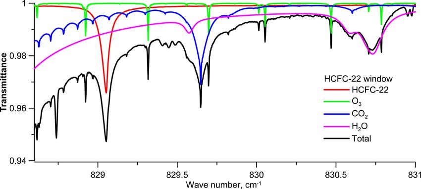
A. Polyakov et al.: Measurements of CFC-11, CFC-12, and HCFC-22 atmospheric content                                                5353

Table 1. The main parameters of the inversion of the spectra for deriving the TCs of halocarbons obtained by Polyakov et al.
(2019a, b, 2020b).

   Gas         Microwindow,      Other gases                                         H2 O spectroscopy     Accounting for channeling
                      cm−1                                                                                 (beam)
   CFC-11            830–860     H2 O (profile), CO2 , O3 , HNO3 , COCl2 (columns)   HITRAN 2016           1.12 cm−1 before 2016
   CFC-12         1160–1162      H2 O, O3 , N2 O, CH4 (columns)                      HITRAN 2009           1.26 cm−1 before 2016
   HCFC-22      828.75–829.4     CO2 , O3 , H2 O (columns)                           HITRAN 2009           1.1 cm−1 before 2016

(mercury cadmium telluride, MCT) detector at temperatures
are cooled by liquid nitrogen (e.g., Hudgins et al., 1993;
Lynch, 2006). Absorption of radiation by AWI depends on
its thickness, which increases during the measurement pe-
riod and decreases during the period of inactivity of the in-
strument when the detector is not cooled. In addition, the wa-
ter vapor from the atmospheric air gradually (on a monthly
scale) seeps into the evacuated zone of the instrument and
also leads to an increase in the AWI thickness. To compen-
sate for the BSS curvature due to the AWI thickness, we use
a second-degree polynomial implemented in the SFIT4 code.
To account for the variability in the AWI thickness, we turn
on the coefficient at the quadratic term of the polynomial
(hereinafter, curvature value) and limit its a priori variability
to avoid the “over-freedom” of the solution. We minimized
the intraday variability in CFC-11 TCs in a series of spectra
                                                                      Figure 1. A dependence of the differences in CFC-11 TCs, derived
processing and, in the first step, obtained the a priori thick-
                                                                      without and with taking the continuum on precipitable water during
ness of the AWI (0.3 µm for F3; 0.9 µm for f6) with the a
                                                                      2018 into account.
priori curvature value of zero. In the next step, we optimized
the value of a priori curvature uncertainty as 10−6 for both
filters.                                                              on water vapor TCs with and without considering the wa-
    The water vapor continuum makes a significant contribu-           ter vapor continuum. This dependence may misinterpret, for
tion to radiation attenuation by the atmospheric water vapor          example, the results of the analysis of CFC-11 seasonal vari-
(Mlawer et al., 2012). Our calculations have shown that radi-         ations (see Sect. 3.3), the maximal amplitude of which does
ation absorption by the water vapor continuum in the consid-          not exceed 3 %, while the maximal difference in TCs due to
ered spectral region under conditions at the St. Petersburg site      the water vapor continuum is close to 0.2×1015 cm−2 , which
can significantly exceed 50 %. For a 30 cm−1 window, the              is more than 4 %.
selectivity of the continual uptake is sufficient to influence           Thus, for CFC-11 processing, we take into account the
the spectra-processing results. To calculate the water vapor          STF, AWI variability, and water vapor continuum. Figure 2
continuum, we use a freely distributed computer code (AER,            highlights their contribution to the distortion in BSS. The ex-
2017) and the daily profiles of water vapor independently de-         pression for the monochromatic transmission function P (ν)
rived from the FTIR measurements (Virolainen et al., 2017).           can be written as Eq. (1), as follows:
The code (AER, 2017) calculates the spectral dependence
of the continuum absorption of radiation by a homogeneous             P (ν) = exp(−τ (ν)),                                          (1)
layer of the atmosphere. We used this code to integrate the
optical thickness of all atmospheric layers, based on the same        where, in the following:
profiles of pressure and temperature that were used in SFIT4.
As a first approximation, the contribution of the water vapor         τ (ν) = τFilter (ν) + τIce (ν) + τCont (ν) + τCFC-11 (ν)
continuum to absorption is proportional to the water vapor
                                                                              + τOGases (ν).                                        (2)
partial pressure squared, and it can only be detected in a very
humid atmosphere. We estimated the contribution of the wa-
                                                                         Terms correspond to contribution to optical depth by op-
ter vapor continuum numerically by analyzing spectra with
                                                                      tical filter (IRWG NDACC f6), ice on the cooled detector,
and without considering the spectra measured in 2018. Fig-
                                                                      continuum attenuation, CFC-11, and other gases. Figure 2
ure 1 depicts a dependence of differences in CFC-11 TCs
                                                                      depicts the first four terms of the right-hand side of Eq. (2).

https://doi.org/10.5194/amt-14-5349-2021                                                 Atmos. Meas. Tech., 14, 5349–5368, 2021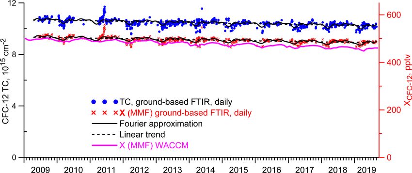
5354                            A. Polyakov et al.: Measurements of CFC-11, CFC-12, and HCFC-22 atmospheric content

Figure 2. Nonlinearity of optical depth components 1 = τ (ν) −
(τ830 + (τ860 − τ830 )(ν − 830)/30). As on 29 July 2018, where the
solar zenith angle is 60◦ .

                                                                     Figure 3. Dependence of the TCs intraday variability in the regu-
   We may conclude that nonlinearities in the first three of         larization parameter α.
them are too considerable to be taken into account when
CFC-11 content is estimated from a spectrum.
                                                                     ments is less and DFS is close to 1; therefore, large values
2.3    Method for solving the inverse problem                        of the parameter α and the corresponding requirements for
                                                                     smoothness do not contradict the information contained in a
For solving the inverse problem, we used the T−Ph approach           spectrum.
presented by Tikhonov (1963) and Phillips (1962). The use               For CFC-11, the minimum of the intraday variability of
of the first-order T−Ph regularization (Tikhonov, 1963) for          0.589 % is reached asymptotically for all values of α not less
retrieving the TCs of trace gases is described in detail, for        than 85, and the DFS at α = 85 differs from 1 (DFS = 1.08).
example, by Sussmann et al. (2011).                                  For CFC-12, the optimal value of the regularization pa-
   For the optimization of the regularization parameter α, we        rameter α = 85, this value corresponds to the intraday SD
used a technique based on minimizing the intraday variabil-          minimum of 0.382 %, and DFS totals 1.18. For HCFC-22,
ity in TCs suggested by Sussmann et al. (2011). In addition,         the minimum of intraday variability of 0.398 % is reached
we analyzed the residuals (χ 2 ) and values of DFS. For the          asymptotically for all values of α, starting from 3 × 10³ , the
analysis of the regularization parameter, we used spectro-           DFS for all these values amounts to 1.00, and both param-
scopic measurements from 2017, which were characterized              eters do not change for α greater than 3 × 10³ . This can be
by a fairly stable quality of measurements, a low noise level,       interpreted as a complete absence of the information on the
and a possibly more uniform distribution of measurements             vertical profile of HCFC-22 in spectral measurements; thus,
throughout the year, including the winter months. Addition-          we may obtain information on the first guess profile multi-
ally, the year 2017 was chosen due to the measurements with          plier only (profile scaling approach).
the f6 filter, which is used at other sites in the IRWG NDACC           Since DFS is close to unity for all three gases, we can con-
network. The year 2015 was chosen for testing the F3 filter;         sider a profile scaling approach for solving the inverse prob-
calculations demonstrated that values of α that are optimal          lem. However, it turned out that, although the SFIT4 core
for the f6 filter in 2017 are also optimal for the F3 filter.        solves the problem, a Python script for performing the batch
   Figure 3 depicts the RMS intraday variability in TCs of           processing and estimating errors does not work in this case.
target gases as a function of α for 2017. The presence of            Moreover, if profile scaling is used for all gases considered
a pronounced minimum for CFC-12 is due to larger infor-              (see Table 1), then the mass processing is not performed.
mation content of the spectral measurements with respect             If at least one gas (i.e., H2 O) is retrieved as a profile, then
to CFC-12 abundancies compared to CFC-11 and HCFC-22                 mass processing is performed but error estimates are not cal-
(DFS is 1.2 for CFC-12, 1.05 for CFC-11, and 1.0 for HCFC-           culated. We compared the two approaches by analyzing all
22; see Table 3). The reason for this is a weak absorption of        spectra measured in 2018 (681 measurements over 80 d) for
interfering gases in the spectral range for CFC-12 retrievals.       CFC-11 retrieval. The average difference between the TCs
Thus, for CFC-12, an increase in the regularization param-           derived from profile scaling and T−Ph approaches for this
eter, which tightens the requirement for spectrum smooth-            set of measurements is 0.016 × 1015 cm−2 or 0.33 %, and the
ness, leads to the suppression of useful information on the          SD of the difference is 0.012 × 1015 cm−2 or 0.26 %, which
gas vertical structure contained in a spectrum. Consequently,        is significantly less than the measurement errors estimated.
the intraday variability in retrievals is increasing. For CFC-11     Therefore, to avoid problems with batch processing and er-
and HCFC-22, the information content of spectral measure-            ror analysis, we chose the T−Ph approach.

Atmos. Meas. Tech., 14, 5349–5368, 2021                                               https://doi.org/10.5194/amt-14-5349-2021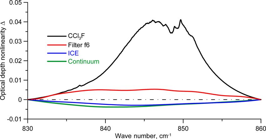
A. Polyakov et al.: Measurements of CFC-11, CFC-12, and HCFC-22 atmospheric content                                          5355

   Using the T−Ph approach and choosing the regulariza-            the retrieval; it characterizes the quality of fitting the mea-
tion parameter based on minimizing the intraday variabil-          sured spectra with the calculated one. Ideally, the spectral
ity of TCs, we obtained DFS = 1 for HCFC-22; the DFS               residual should be equal to the measurement’s noise level.
value of other two gases is close to 1 (1.05 and 1.20; see         For target gases, the mean values of the spectral residuals
Table 3). Prignon et al. (2019) reported the higher values of      vary from 0.34 % to 0.52 %, depending on the gas; it cor-
DFS (DFS = 1.97) caused by T−Ph regularization with the            responds to the signal-to-noise ratio (SNR) values of 209,
parameter α = 9 and a low atmospheric water vapor content          280, and 327 for CFC-11, CFC-12, and HCFC-22, respec-
above the mountain (3580 m a.s.l.) site of Jungfraujoch.           tively. Since the spectrum in residual calculations has been
                                                                   normalized to the unit, SNR and residual are the recipro-
                                                                   cal values, i.e., SNR = 1/residual. Comparing these values
3     Results and analysis                                         to the preliminary determined mean SNR in the opaque spec-
                                                                   tral range (364, 351, and 324 in the same order of gases), we
The techniques described above were applied to processing          see that, for CFC-11 and CFC-12, they are slightly less and,
the entire archive of spectral measurements at the NDACC           for HCFC-22, they are nearly the same. This means that, for
site of St. Petersburg for the period of 2009–2019.                CFC-11 and CFC-12, the radiative transfer model and a set
                                                                   of parameters used, although satisfactory, do not ideally de-
3.1    The filtering of the results                                scribe the absorption of radiation by the atmosphere and the
                                                                   observational system, whereas, for HCFC-22, the retrieval
Table 2 presents a number of statistical characteristics and       technique works in the best way.
the assessment of total errors for target gases.                      Rows 3–7 of Table 3 present the characteristics of the tar-
   The first row in Table 2 shows the total number of spec-        get gases retrievals, TCs, and Xgas. Row 3 shows the means,
tra/days for which the TCs have been obtained. Although the        and row 4 shows the RMS intraday variability in Xgas, which
total number of spectra taken for SFIT4 processing was 4804        can be interpreted as being their precision. Comparison of the
(see Sect. 2.1), we had to remove 31 spectra for CFC-11 as         RMS intraday variability values with the estimates of the ran-
they were measured with the incorrect filter (F3 instead f6        dom error (row 11 of Table 4) demonstrates that, for HCFC-
and vice versa). The retrieval technique for CFC-11 is very        22, the intraday variability practically coincides with the to-
sensitive to the correctly defined filter (see Sect. 2.2 on BSS    tal random error. The other two gases show a significantly
for CFC-11). Thus, the number of spectra for CFC-11 was            different ratio, and the intraday variability is noticeably less
4773. The number of spectra is different for different gases,      than the random error (i.e., 0.76 % vs. 3.08 % for CFC-11 and
since the solution of the inverse problem algorithm imple-         0.58 % vs. 2.40 % for CFC-12). Therefore, the random error
mented in SFIT4 does not always provide a solution. The            has a significant component of a systematic nature during 1 d
total number of spectra suitable for processing for over more      of measurements but randomly changes from 1 d to another.
than 10 years of observations (from March 2009 to August           It should be noted that the temperature profile changes in-
2019) is about 4500–4800, measured over about 720 d. Thus,         significantly during a day, so the intraday variability in Xgas
on average, the FTIR measurements at the St. Petersburg site       includes the corresponding component and exceeds the con-
are carried out for 68 d yr−1 . Such a relatively small number     tribution of a total random noise of spectroscopic measure-
of days of measurements is primarily due to the latitude and       ments. Thus, the resulting error budget estimates and the in-
climatic features of the site.                                     traday variability in the results are mutually consistent.
   As we observed some outliers in the HCFC-22 TCs time               The DFS (row 5) for all gases is close to 1, which is pri-
series before 2016, we discarded the TCs values that differed      marily due to the T−Ph approach and the selection of the
from the approximating line (trend) by more than three SD          regularization parameter α, based on minimizing the intra-
values. A total of 219 measurements were excluded; thus,           day variability in the gas TCs. Row 6 of Table 3 shows
the HCFC-22 spectra number is less then spectra numbers for        the trend values estimated in accordance with a method de-
two other gases. In the next step, we filtered the retrieved TCs   scribed by Gardiner et al. (2008). This method is based on the
using the following criterion: the deviation from the mean         RMS approximation of the variability in gas concentrations
statistical characteristics presented in Table 2 should not be     by a three-term segment of the Fourier series and bootstrap
greater than 2 × SD. Details of this selection are shown in        method of confidence intervals assessment for 95 % prob-
Table B1 of Appendix B.                                            ability. Finally, row 7 shows the RMS difference between
   Table 3 gives some statistics for target gases measure-         Xgas and the trigonometric Fourier series used to estimate
ments after filtering the retrievals. The general information      its temporal variability. For CFC-11 and CFC-12, these val-
on the spectra analyzed is given in row 1 (the number of           ues are close to the random error (2.8 % vs. 3.08 % and 2.1 %
measurement days and single measurements) and in row 2             vs. 2.40 %), which indicates an adequate description of their
(the spectral residuals). The number of days is close to 670,      variability by the Fourier series. At the same time, for HCFC-
and the number of the retrieved TCs is close to 3900 for each      22, the RMS difference is 5.3 %, which exceeds the random
gas. The spectral residual is the most important parameter of      error of 3.7 %, and the HCFC-22 variability involves some

https://doi.org/10.5194/amt-14-5349-2021                                             Atmos. Meas. Tech., 14, 5349–5368, 2021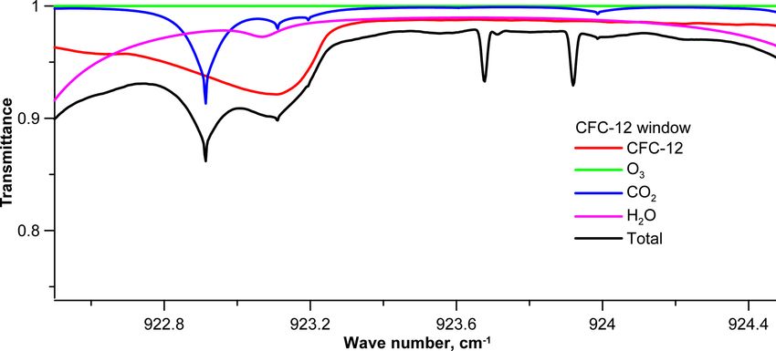
5356                                     A. Polyakov et al.: Measurements of CFC-11, CFC-12, and HCFC-22 atmospheric content

Table 2. Summary of the statistics for retrieved halocarbons TCs before filtering. The values after the “±” sign indicate the standard deviation
(SD). DFS is the number of degrees of freedom for signal.

                                   No.      Parameter                       CFC-11           CFC-12     HCFC-22
                                   1        No. of spectra/days            4773/720      4768/718       4585/714
                                   2        RMS (%)                      0.53 ± 0.46   0.45 ± 0.55    0.40 ± 0.29
                                   3        Total systematic error (%)   7.60 ± 0.18   2.26 ± 0.16    5.75 ± 0.08
                                   4        Total random error (%)       3.23 ± 0.77   2.56 ± 0.94    4.18 ± 2.66
                                   5        Intraday SD (%)                     1.35          0.70           5.63
                                   6        DFS                          1.07 ± 0.09   1.20 ± 0.05    1.00 ± 0.00

Table 3. Summary of the statistics for retrieved halocarbon TCs after filtering.

           No.     Parameter                                                      CFC-11                CFC-12      HCFC-22
           1       No. of spectra/days                                           3864/678              3912/664     3855/663
           2       RMS (χ 2 )                                                  0.52 ± 0.18           0.40 ± 0.16    0.34 ± 0.13
           3       Mean TC (cm−2 ; Xgas; pptv)                           4.75 × 10¹⁵ (225)    10.42 × 10¹⁵ (493)    5.04 × 10¹⁵ (238)
           4       Intraday SD of Xgas (%)                                            0.76                  0.58    3.74 (4.54/2.32)∗
           5       DFS                                                         1.05 ± 0.06           1.20 ± 0.05    1.00 ± 0.00
           6       Trend (% yr−1 )                                           −0.40 ± 0.07          −0.49 ± 0.05     2.12 ± 0.13
           7       Total SD of Xgas (%; except Fourier approx.)                        2.8                   2.1    5.3
         ∗ Before/after February 2016.

other components besides the trigonometric Fourier series.                    matrix; the corresponding column for these elements is pre-
The reason for such behavior of HCFC-22 is a reduction in                     sented in Table 4. For the temperature profile (row 1) below
its use during the period analyzed that leads to a decrease in                40 km, where the profiles of the target gases are derived, the
its growth rate. As a result, the representation of its variabil-             absolute value of the temperature systematic error totals 1–
ity in the form of a linear increase and seasonal variations,                 2 K, and the random error totals 2–4 K, depending on the al-
represented by trigonometric Fourier series (see Sect. 3.2),                  titude. For other parameters, the relative errors are indicated
cannot be accurate. Polyakov et al. (2020a) demonstrated                      in other rows of Table 4. In addition to fixed parameters, two
the decrease in a growth rate of HCFC-22 abundancies over                     types of parameters are fitted in the retrieval process, namely
St. Petersburg in the past decade.                                            (1) the retrieval parameters, including a number of instru-
   The SFIT4 software provides the calculation of the er-                     mental parameters, such as BSS (a slope for all three gases
ror budget based on the Rodgers (2000, Chap. 3) approach                      and a curvature for CFC-11), along with instrumental line
for each measurement. Rodgers (2000, Eq. 3.16) considers                      shape, channeling before 2016, zero level uncertainty, etc.,
the four components of the measurement error, namely the                      and (2) the content of interfering atmospheric gases listed
smoothing error, model parameter error, forward model er-                     in Table 1 (column 3, other gases), for which the absorp-
ror, and the retrieval noise. To estimate the mean smoothing                  tion lines overlap with the lines of the target gas. Their con-
error, it is necessary to have real covariance matrices of the                tribution to the error budget is shown in rows 8 (interfering
gas vertical profiles, which are not available; therefore, we                 species) and 9 (retrieval parameters). We assume that the for-
cannot estimate this component of the error. We can only as-                  ward model error (Rodgers, 2000, Eq. 3.16) is negligible in
sume that it is small because, due to their long lifetime, we                 our retrieval. The retrieval noise shown in row 10 indicates
expect nearly constant volume mixing ratio (VMR) profiles                     the error corresponding to the spectra measurement noise.
of the target gases in the troposphere. Prignon et al. (2019)                    Row 11 in Table 4 demonstrates that, for CFC-11
showed that the smoothing error for HCFC-22 is rather small                   and HCFC-22, total systematic errors are relatively large,
(0.3 %). The model parameter error is caused by the inaccu-                   amounting to 7.61 % and 5.75 %, and these values are almost
racies in setting the parameters describing the instrument and                entirely due to the uncertainty in the spectroscopic informa-
the state of the atmosphere.                                                  tion on the intensities of pseudo-lines (row 3 of Table 4). For
   To calculate the terms of the model parameter error, which                 CFC-12, the total systematic error is estimated as 2.2 %, and
are shown in rows 1–7 of Table 4, Eq. (3.18) in Rodgers                       the main source of this error is the uncertainty of the tem-
(2000) was used. For this equation, it is necessary to first set              perature profile (row 1 of Table 4). Note that the value of the
the uncertainties of various parameters which are taken into                  total systematic error is slightly variable, and its SD is maxi-
account. Rodgers (2000) enters them as elements of the Sb                     mal for CFC-11, which comprises 0.16 %. The total random

Atmos. Meas. Tech., 14, 5349–5368, 2021                                                         https://doi.org/10.5194/amt-14-5349-2021
A. Polyakov et al.: Measurements of CFC-11, CFC-12, and HCFC-22 atmospheric content 5357
error and its variability is maximal for HCFC-22. The main analyzed as a seasonal data variability. Figures 4–6, in ad-
contribution to it is made by the spectral measurement er- dition to the daily mean values of Xgas and TC, also show,
ror, which is caused by the low absorption of the solar radi- with a dashed line, the linear trend a + bt and, with a solid
ation by this gas. The random components of the total error black line, the result of approximating the measurement data
for other two gases, 3.08 % and 2.40 %, are more stable, and by the trigonometric Fourier series in Eqs. (3) and (4). Fig-
their main source is the error in the temperature profile (see ure 4 demonstrates a pronounced periodicity of the results,
row 1). It should be noted that the filter used has a signifi- showing the seasonal variation in both the TCs and Xgas of
cant effect on the errors and variability in the HCFC-22 TCs. CFC-11. A similar periodicity is also observed in satellite
When switching to the IRWG NDACC f6 filter in February measurements and in the WACCM data. As expected, Xgas
2016, the intraday variability in the results (row 4 of Table 3) exhibit a slightly smaller scatter than TCs. Note that, start-
decreased by approximately 2 times, and the random compo- ing from April 2019, there is a sharp increase in the concen-
nent of the total error (row 11 of Table 4) decreased by 1.4 %, trations of CFC-11. At present, we have no way of explain-
mainly due to the error of spectroscopic measurements. Due ing whether such growth is objectively presented or caused
to channeling, the use of the F3 filter before February 2016 by peculiarities in the operation of the instrument. At the
leads to a large scatter in retrieval results (see Sect. 2.1). same time, this growth noticeably affects the trend estimates.
Therefore, when calculating the trends of CFC-11 TCs and
3.2 Analysis Xgas, we limited the CFC-11 time series to April 2019, leav-
ing the analysis of the reasons for this feature outside the
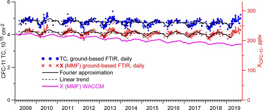
Figures 4–6 show the results in a form of the daily means scope of this study.
of both TCs and Xgas. The TC values directly represent the CFC-12 measurements (Fig. 5) show significantly differ-
results of spectra inversion, while Xgas values are calculated ent results. First of all, the comparison of Figs. 4 and 5 and
by dividing the gas total column by the dry air total column. estimates of the intraday variability and measurement uncer-
The analysis of Xgas values avoids the influence of the sur- tainties of these gases demonstrate that the TCs and Xgas
face pressure and humidity variability, and thus, these values of CFC-12 show less scatter than that of CFC-11, except for
are more stable. To analyze the variability in target gases on some isolated anomalies. The seasonal variability in these
a scale of both long-term trends and seasonal variability, we values for CFC-12 is noticeably less than that for CFC-11.
used the approach implemented by Gardiner et al. (2008) for We also note that, moving from TCs to Xgas, the deviations
assessing the trends, which is based on the approximation of in the results from the approximating segment of the Fourier
a series of data by expansion on a finite-dimensional basis; series decrease significantly. Variations in surface pressure
see Eq. (3). and water vapor TCs make a significant contribution to the
variability in CFC-12 TCs, which indicates small changes
F (t) ≈ a + bt + c1 f1 (t) + c2 f2 (t). . . + ck fk (t). (3)
in its VMR profile. We analyze these factors in detail in
In Eq. (3), F (t) is a dependence approximated by the expan- Sect. 3.3.
sion, in our case represented by discrete measurement data, Having considered the results of measurements of HCFC-
t is time (years), a is the constant, and b is the linear term 22 daily means, we observed a large variability consistent
coefficient that is equal to a trend value. ci , i = 1, and k are with a large random component of the total error estimates
the coefficients, k is the number of coefficients, and fi (t) are (see Table 4). There are also noticeable seasonal variations.
the basis functions. Due to the annual cyclical nature of at- At first glance, the filter change in February 2016 clearly
mospheric processes, a trigonometric Fourier series with a manifests itself in a change in the data scatter, but in 2016,
maximum period of a year is used, which corresponds to the the scatter looks no less than in previous years and sharply
basis functions in Eq. (4), as follows: decreases in 2017 and later. Noteworthy is the observed ces-
sation of the increase in HCFC-22 values starting from 2018,
f2i−1 (t) = cos(2π it), f2i (t) = sin(2π it), i = 1, m, (4) previously described by Polyakov et al. (2020a). We also ob-
served an increase in the scatter of the results for all three
where m = 3 or, which is the same, k = 6. Let us write gases in 2013 due to a decrease in the SNR values caused by
Eq. (3) in the form of Eq. (5), highlighting the nonlinear part the degradation of the tracking system mirror.
S(t) (Eq. 6). Table 5 presents trend estimates for Xgas time series using
two different methods described by Gardiner et al. (2008)
F (t) ≈ a + bt + S(t), (5) and Timofeev et al. (2020). Gardiner et al. (2008) model the
where, in the following: intra-annual variability in terms of a Fourier series, and Tim-
ofeev et al. (2020) use monthly mean values of the consid-
S(t) = c1 f1 (t) + c2 f2 (t). . . + ck fk (t). (6) ered period to describe a seasonal cycle. In both methods,
trends are estimated by subtracting the seasonal variability
S(t) can be considered as being a periodic component of the from initial time series. In the first method, we consider pe-
measurement data time sequence, and its one period can be riodicities of 4 months and larger; in the second method, the
https://doi.org/10.5194/amt-14-5349-2021 Atmos. Meas. Tech., 14, 5349–5368, 20215358 A. Polyakov et al.: Measurements of CFC-11, CFC-12, and HCFC-22 atmospheric content
Table 4. Error budget for retrieved halocarbons TCs. The relative uncertainties of spectroscopic parameters are 7 %, 1 %, and 5 % for CFC-11,
CFC-12, and HCFC-22, respectively. Sb means the a priori imprecision of parameters.
No. Gas CFC-11 CFC-12 HCFC-22
TCs error, %
Parameter Sb , % Systematic Random Systematic Random Systematic Random
1 Temperature 2.29 ± 0.25 2.56 ± 0.30 1.96 ± 0.15 1.96 ± 0.12 1.72 ± 0.07 1.50 ± 0.06
2 SZA 0.1 ± 0.5 0.20 ± 0.17 1.03 ± 0.84 0.22 ± 0.18 1.09 ± 0.89 0.25 ± 0.25 1.27 ± 1.27
3 Target line intensity 7/1/5 7.02 ± 0.28 0.45 ± 0.49 5.04 ± 0.45
4 Target temperature
dependence of
line width 7/1/5 0.00 ± 0.00 0.27 ± 0.05
5 Target air broadening 7/1/5 0.02 ± 0.03 0.61 ± 0.14 2.16 ± 0.24
of line width 7/1/5 0.02 ± 0.03 0.61 ± 0.14 2.16 ± 0.24
6 H2 O spectroscopy 10 1.45 ± 0.57 0.31 ± 0.31 0.25 ± 0.35
7 Zshift 1±1 1.03 ± 0.10 1.03 ± 0.10 0.12 ± 0.01 0.25 ± 0.03 0.10 ± 0.01 0.20 ± 0.02
8 Interfering species 0.04 ± 0.04 0.02 ± 0.01 0.19 ± 0.12
9 Retrieval parameters 0.12 ± 0.07 0.02 ± 0.00 0.29 ± 0.05
10 Spectra measurement 0.29 ± 0.13 0.20 ± 0.03 2.66 ± 1.62
noise (3.3/1.8)∗
11 Total 7.61 ± 0.16 3.08 ± 0.36 2.24 ± 0.14 2.40 ± 0.54 5.75 ± 0.08 3.70 ± 1.29
(4.32/2.92)∗
∗ Before/after February 2016. SZA is the solar zenith angle.
Figure 4. Daily mean TCs and Xgas of CFC-11. The T−Ph parameter α = 85.
monthly mean values account for periodicities from 1 month. tainties; however, due to substantially irregular FTIR mea-
The estimation of the width of the confidence interval of the surements, it was difficult to estimate it.
trend value for Gardiner’s approach is carried out using the Table 5 demonstrates that the differences between two
bootstrap method; for Timofeev’s method, it is calculated methods remain within the 95 % confidence interval, i.e.,
on the basis of a theoretical statistical approach. We do not they are not significant.
take the autocorrelation that can be presented in long-lived
Xgas time series into account. Santer et al. (2000) demon- 3.3 Comparison with independent data
strated that neglecting the autocorrelation in a time series
could affect the trends estimates and underestimate uncer- We compared the FTIR results at the St. Petersburg site with
the data of measurements and modeling. There are three
Atmos. Meas. Tech., 14, 5349–5368, 2021 https://doi.org/10.5194/amt-14-5349-2021A. Polyakov et al.: Measurements of CFC-11, CFC-12, and HCFC-22 atmospheric content 5359
Figure 5. Daily mean TCs and Xgas of CFC-12. Filtered results of the T−Ph parameter α = 85.
Figure 6. Daily mean TCs and Xgas of HCFC-22. Filtered results of the T−Ph parameter α = 3 × 10³ .
Table 5. Estimated trends of Xgas derived from the FTIR measure- 11, CFC-12, and HCFC-22 equal 234, 517, and 237 pptv
ments at the St. Petersburg site in 2009–2019. (parts per trillion by volume), whereas the FTIR Xgas mea-
surements show 225, 493, and 252 pptv means, respectively.
Gas Gardiner et al. (2008) Timofeev et al. (2020) The trend values (Table 6; columns 2 and 4) for the GVMR
CFC-11 −0.40 ± 0.07 −0.39 ± 0.08 data are −0.53, −0.59, and 2.0 % yr−1 ; for the FTIR data,
CFC-12 −0.49 ± 0.05 −0.46 ± 0.05 they are −0.38, −0.48, and 2.0 % yr−1 for CFC-11, CFC-12,
HCFC-22 2.12 ± 0.13 2.22 ± 0.14 and HCFC-22, respectively. Taking into account the spatial
discrepancy, the different nature of the measured quantities
and the different measurement conditions (background con-
ditions on the Atlantic coast and measurements near the large
sources of data for the concentration of halocarbons in the agglomeration of St. Petersburg), the agreement between the
atmosphere. First, the in situ measurements at the surface mean values and the trends can be considered satisfactory.
(carried out exactly by the in situ and flask methods) are It should be noted that the differences in trend estimates
available from the AGAGE (Dunse et al., 2005) and HATS do not go beyond the differences in trend values obtained
(Montzka et al., 1993) observational networks; the data are by other researchers. Zhou et al. (2016) obtained trends of
regularly updated at ftp://ftp.cmdl.noaa.gov/hats (last access: −0.86 % yr−1 , −0.76 % yr−1 , and 2.84 % yr−1 for the period
28 June 2020). Measurements are carried out at fixed loca- 2009–2016; WMO (2018) indicated that averaged VMRs
tions, the closest of which is Mace Head, Ireland (MHD), at for 2015 comprised 229.2–231.1, 515.3–519.7, and 233.0–
a distance of 2500 km and 6.6◦ south of the St. Petersburg 238.0 pptv, and the trends for the period 2010–2016 were
site. The mean values and the trends of Xgas were calcu- −0.70 % yr−1 , −0.47 % yr−1 , and 2.54 % yr−1 for CFC-11,
lated from the FTIR data and from the MHD site near-ground CFC-12, and HCFC-22, respectively. Taking into account the
data for the period (2009–2019) for all three gases. The re- decrease in both the rate of decay of CFC-11 and the rate of
sults are shown in Table 6 in columns 1 and 3. The mean growth of HCFC-22 (e.g., Polyakov et al., 2020a), the agree-
near-ground VMRs (GVMRs) at the MHD site for CFC-
https://doi.org/10.5194/amt-14-5349-2021 Atmos. Meas. Tech., 14, 5349–5368, 20215360 A. Polyakov et al.: Measurements of CFC-11, CFC-12, and HCFC-22 atmospheric content ment of both concentrations and trend values seems to be to the different physical nature of the compared quantities. satisfactory. The satellite data do not take into account the lower tropo- The second source of information on the halocarbons con- spheric layers, where the influence of anthropogenic pollu- tent is the satellite measurements, presented most fully for tion sources is the greatest. Therefore, analyzing the trends target gases by the ACE-FTS instrument data (for which ver- and deriving from this that the background values of the sion 4 is described by Boone et al., 2020). The ACE-FTS is a VMRs for atmospheric CFC-11 and CFC-12 (in situ and high spectral resolution (0.02 cm−1 ) Fourier transform spec- satellite) are falling faster than the FTIR Xgas in the industri- trometer operating from 2.2 to 13.3 µm (750–4400 cm−1 ), ally developed European part of Russia (near the megacity of based on a Michelson interferometer. The instrument is a St. Petersburg), we may assume that some sources of CFC- main payload on board the SCISAT-1 satellite, with a drift- 11 and CFC-12 exist somewhere there. The absolute values ing orbit, an inclination of 73.9◦ , and an altitude of 750 km. of CFC-11 and CFC-12 FTIR Xgas are smaller than that of Working primarily in the solar occultation mode, the satel- the in situ and satellite measurements, but this may only be lite provides information on vertical profiles (typically 10– due to the uncertainty of the spectroscopy used (see the esti- 100 km) for temperature, pressure, and the VMRs of dozens mates of the systematic in Table 4; row 3). of atmospheric gases over the latitudes of 85◦ N to 85◦ S. Figure 7 depicts seasonal variation functions S(t), in The lower boundary of the retrieved profiles does not fall Eq. (6), for three gases and for four types of data, i.e., near- below 6 km, but, as a rule, it is above 7–8 km, and the er- ground VMR (GVMR) at the MHD station, satellite mean rors at the lower level may be greater than in the rest of the VMR (SVMR) 8–12 km (55–65◦ N), the Xgas by FTIR mea- profile. Therefore, we used, for comparisons only, the pro- surements (Xgas), and the Xgas from the WACCM (WX- files in which the data were available above 7 km and ana- gase). lyzed the average satellite VMRs (SVMR) in the 8–12 km There are some fundamental differences between local layer to reduce the random error. For comparison, we se- surface and remote sensing measurements (satellite and lected the ACE-FTS measurements closer than 500 km from ground-based FTIR). First, surface measurements are per- the St. Petersburg site. In 2009–2019, there are only 47 d formed regularly and frequently, resulting in stable averages. of SVMR measurements for CFC-11 (mean 233 pptv; trend Second, they are unaffected by variations in pressure and −0.68 ± 0.23 % yr−1 ), 47 d for CFC-12 (mean 521 pptv; tropopause height. And, finally, the surface data used were trend −0.52 ± 0.16 % yr−1 ), and 46 d for HCFC-22 (mean obtained in close to background conditions. Therefore, Fig. 7 240 pptv; trend 2.0 ± 0.5 % yr−1 ). The results are shown in demonstrates the low seasonal variability in the GVMR, columns 7 and 8 of Table 6. Due to the peculiarity of the which is within tenths of a percent for CFC-11 and CFC- orbit and the weather conditions at the St. Petersburg site, 12 and within 0.7 % for HCFC-22. At the same time, a no- SCISAT-1 measurements are available on rare occasions; ticeable seasonal variation in the FTIR Xgas and the SVMR during 10 years, we have not found more than 47 measure- values for all three gases and of the WACCM Xgas for CFC- ments closer than 500 km to the St. Petersburg site. How- 11 and CFC-12 are observed. The maximal amplitude of the ever, the 95 % probability intervals show the reliability of the variability reaches 4 % for CFC-11, slightly exceeds 3 % for trend estimates, using the bootstrap method by Gardiner et HCFC-22, and is close to 2 % for CFC-12. For all three gases, al. (2008). As one can see, by comparing columns 1 and 7 of seasonal variations in SVMR and Xgas are qualitatively and Table 6, the confidence intervals of the means overlap, i.e., quantitatively similar; in spring (March–April), there is a the difference in the mean values is not significant only for minimum, and in late summer or autumn (August–October), HCFC-22, and for both CFC-11 and CFC-12, the SVMR is there is a maximum. At the same time, there are some dif- significantly greater than the FTIR Xgas; the difference totals ferences in the seasonal cycles. For CFC-11, the change in 8 pptv, or 3.5 % for CFC-11 and 28 pptv or 6.3 % for CFC- Xgas is 2–3 months ahead of SVMR, while for HCFC-22 12. To increase the number of data pairs, we analyzed all the autumn maximum shows the same tendency, whereas the ACE-FTS data at all longitudes in the 55–65◦ N latitudinal spring minimum, on the contrary, is observed simultaneously range, including the St. Petersburg site (about 60◦ N). For the for Xgas and SVMR. For CFC-12, the Xgas amplitude is ap- period of the FTIR measurements, the SVMR data include proximately half that for two other gases; the spring min- 1113 measurements for CFC-11, with the mean of 235.3 pptv imum of Xgas, on the contrary, is observed before that of and the trend value of −0.63 % yr−1 , 1120 measurements SVMR, and the autumn maxima coincide. For CFC-12, a for CFC-12 (526.4 pptv, −0.58 % yr−1 ), and 1111 measure- second maximum in the Xgas seasonal cycle is observed in ments for HCFC-22 (239.5 pptv, 2.2 % yr−1 ; see columns 5 the early summer. WXgas for CFC-11 and CFC-12, on the and 6 of Table 6). whole, show a qualitatively and quantitatively similar sea- With a 20 times larger data set, the confidence intervals sonal variability to Xgas and SVMR, while, on the contrary, for the trends for the latitudinal range are much narrower for HCFC-22, the changes in WXgas are significantly less than for a circle with a radius of 500 km; thus, differences (less than 1 %) than that of Xgas and SVMR. In general, we in the SVMR trends vs. FTIR Xgas trends for CFC-11 and can conclude that Xgas, SVMR, and WXgas show qualita- CFC-12 become significant. Such a discrepancy may be due tively similar seasonal variation, with some quantitative dif- Atmos. Meas. Tech., 14, 5349–5368, 2021 https://doi.org/10.5194/amt-14-5349-2021
You can also read