Comparison and evaluation of anthropogenic emissions of SO2 and NOx over China
←
→
Page content transcription
If your browser does not render page correctly, please read the page content below
Atmos. Chem. Phys., 18, 3433–3456, 2018
https://doi.org/10.5194/acp-18-3433-2018
© Author(s) 2018. This work is distributed under
the Creative Commons Attribution 4.0 License.

Comparison and evaluation of anthropogenic emissions
of SO2 and NOx over China
Meng Li1,3,a , Zbigniew Klimont2 , Qiang Zhang1 , Randall V. Martin4 , Bo Zheng3 , Chris Heyes2 , Janusz Cofala2 ,
Yuxuan Zhang1,a , and Kebin He3
1 Ministry  of Education Key Laboratory for Earth System Modeling, Department for Earth System Science,
Tsinghua University, Beijing, China
2 International Institute for Applied Systems Analysis (IIASA), Laxenburg, 2361, Austria
3 State Key Joint Laboratory of Environment Simulation and Pollution Control, School of Environment,

Tsinghua University, Beijing, China
4 Department of Physics and Atmospheric Science, Dalhousie University, Halifax, Canada
a now at: Max-Planck Institute for Chemistry, Mainz, Germany

Correspondence: Meng Li (m.li@mpic.de) and Bo Zheng (bo.zheng@lsce.ipsl.fr)

Received: 9 July 2017 – Discussion started: 4 August 2017
Revised: 22 January 2018 – Accepted: 6 February 2018 – Published: 8 March 2018

Abstract. Bottom-up emission inventories provide primary         For NOx , negative biases in bottom-up gridded emission
understanding of sources of air pollution and essential input    inventories (−21 % for MIX, −39 % for ECLIPSE) were
of chemical transport models. Focusing on SO2 and NOx , we       found compared to the satellite-based emissions. The emis-
conducted a comprehensive evaluation of two widely used          sion trends from 2005 to 2010 estimated by two inventories
anthropogenic emission inventories over China, ECLIPSE           were both consistent with satellite observations. The inven-
and MIX, to explore the potential sources of uncertainties       tories appear to be fit for evaluation of the policies at an ag-
and find clues to improve emission inventories. We first com-    gregated or national level; more work is needed in specific
pared the activity rates and emission factors used in two in-    areas in order to improve the accuracy and robustness of out-
ventories and investigated the reasons of differences and the    comes at finer spatial and also technological levels. To our
impacts on emission estimates. We found that SO2 emission        knowledge, this is the first work in which source comparisons
estimates are consistent between two inventories (with 1 %       detailed to technology-level parameters are made along with
differences), while NOx emissions in ECLIPSE’s estimates         the remote sensing retrievals and chemical transport model-
are 16 % lower than those of MIX. The FGD (flue-gas desul-       ing. Through the comparison between bottom-up emission
furization) device penetration rate and removal efficiency,      inventories and evaluation with top-down information, we
LNB (low-NOx burner) application rate and abatement ef-          identified potential directions for further improvement in in-
ficiency in power plants, emission factors of industrial boil-   ventory development.
ers and various vehicle types, and vehicle fleet need further
verification. Diesel consumptions are quite uncertain in cur-
rent inventories. Discrepancies at the sectorial and provin-
cial levels are much higher than those of the national total.    1   Introduction
We then examined the impacts of different inventories on
model performance by using the nested GEOS-Chem model.           SO2 and NOx are important precursors of secondary PM2.5 ,
We finally derived top-down emissions by using the retrieved     contributing to severe environmental problems including
columns from the Ozone Monitoring Instrument (OMI) com-          haze and acid rain, and have been shown to be detrimen-
pared with the bottom-up estimates. High correlations were       tal to human health and ecosystems (Seinfeld and Pandis,
observed for SO2 between model results and OMI columns.          2006). China’s anthropogenic emissions have become one
                                                                 of the major contributors to the global budget during the

Published by Copernicus Publications on behalf of the European Geosciences Union.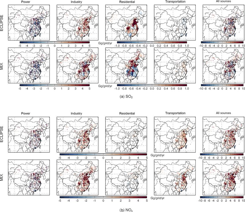
3434                     M. Li et al.: Comparison and evaluation of anthropogenic emissions of SO2 and NOx over China

last decade (Klimont et al., 2013; Hoesly et al., 2018). To          Li et al., 2017), supporting us for explicit comparisons and
support chemical transport modeling and provide scientific           analyses; (d) ECLIPSE (GAINS model, Greenhouse gas-Air
basis for policy-making, several emission inventories cover-         pollution Interactions and Synergies model; Amann et al.,
ing China have been developed (Streets et al., 2003; Ohara           2011) can be representative of the state-of-science global
et al., 2007; Zhang et al., 2007, 2009; Lu et al., 2010, 2011;       emission inventory covering China, and MIX (MEIC model,
Kurokawa et al., 2013; Klimont et al., 2009, 2013; Wang              Multi-resolution Emission Inventory for China; available at
et al., 2014; Li et al., 2017; EDGAR v4.2, available at http:        www.meicmodel.org) represents the regional inventory com-
//edgar.jrc.ec.europa.eu).                                           piled with advanced methods and local data. The methods,
   Bottom-up emissions are estimated through comprehen-              parameters and assumptions of GAINS and MEIC are always
sive parameterization of fuel consumption, industrial produc-        referred to by inventory developers (e.g., Lu et al., 2010; Fu
tion, emission factors and mitigation measures and spatially         et al., 2013; Kurokawa et al., 2013; Zhao et al., 2013). The
allocated to satisfy the chemical and climate model require-         comparisons and validations are important to improve the
ments. Uncertainties of emissions have been qualitatively il-        accuracy of gridded emissions and model performance over
lustrated (e.g., Granier et al., 2011; Saikawa et al., 2017)         China.
or quantitatively analyzed (Streets et al., 2003; Zhao et al.,          Another motivation of this work is to discuss the “fitness”
2011; Guan et al., 2012; Hong et al., 2017), inferring signifi-      of current developed inventories (specifically ECLIPSE and
cant gaps in activity statistics and control measures’ assump-       MIX) and modeling work performed with them for policy-
tions in emission inventories developed for different spatial        relevant discussion. The inventories and the relevant model-
scales (i.e., global, regional, or city scale; Zhao et al., 2015).   ing work are playing an increasingly important role for pol-
   Extensive comparisons of emission inventories have been           icy discussion in Europe and most recently more and more
conducted to illustrate the impacts of variable emissions on         in Asia on different scales. However, there are no systematic
the model simulation results (e.g., Saikawa et al., 2017; Zhou       and officially approved methods and inventories but a variety
et al., 2017). Although they provide important indications on        of scientific products. While a lot of effort has been made
the extent of discrepancies, there are still gaps for applying       to validate emission estimates with measurements, higher
the comparison results to improve the inventory accuracy:            source and spatial resolution of inventories and projections
                                                                     will also serve discussion about how to shape future policies
  1. Comparisons have been conducted for the total anthro-           to reduce impact of air pollution. In this work, we compared
     pogenic sources, instead of by sectors, subsectors, and         the ECLIPSE and MIX emissions over China at a detailed
     sources. Inconsistency of source categories included in         activity-source level. What we focused on in this paper is the
     inventory models were not overviewed or analyzed.               bottom-up comparison detailed to a specific parameter con-
                                                                     tributing to the differences between the two widely used grid-
  2. Few studies go into the comparisons on a specific pa-
                                                                     ded emission inventories (ECLIPSE and MIX), combined
     rameter level because the technology-based framework
                                                                     with top-down validations from the satellite observations. We
     for each inventory was not publicly available.
                                                                     compared the activity rates and emission factors derived from
  3. Top-down and bottom-up comparisons have not been                several key parameters for the largest sources for each sec-
     comprehensively combined to infer the potential uncer-          tor and subsector. Discrepancies in the methodologies used,
     tain parameters for all key sectors.                            data sources, technology penetration assumptions and spatial
                                                                     emission patterns are discussed and illustrated. Furthermore,
   To further improve the accuracy of emission estimation,           we combined the bottom-up comparisons with top-down
we compared and evaluated the global ECLIPSE (Evaluating             evaluations based on observations of the OMI (Ozone Mon-
the Climate and Air Quality Impacts of Short-Lived Pollu-            itoring Instrument) aboard the Aura satellite (Levelt et al.,
tants; Klimont et al., 2017) and MIX Asian (Li et al., 2017)         2006). To our knowledge, this is the first emission inventory
inventories due to the following reasons: (a) Up to the time         assessment work in which parameter-level comparison and
of paper preparation, ECLIPSE and MIX were the only pub-             remote sensing evaluations are combined. OMI data provide
licly accessible gridded emission datasets that include both         essential constraints on emission estimates, spatial distribu-
SO2 and NOx covering China for the period of 2005 and                tions and trends (Wang et al., 2012; Liu et al., 2016). In recent
2010; (b) both inventories have been widely applied in atmo-         work described by Geng et al. (2017), OMI NO2 columns
spheric modeling and policy discussions (e.g., Stohl et al.,         were applied to analyze and evaluate the sensitivities of spa-
2015; Duan et al., 2016; Galmarini et al., 2017; Rao et al.,         tial proxies used in the emission gridding process.
2017); (c) the technology-based framework and compiling                 Methodology and data used are summarized in Sect. 2.
parameters by source categories are obtained for ECLIPSE             Bottom-up comparisons of emissions are illustrated by
and MIX through international collaboration, which is not            decomposing the elements of inventory development in
accessible for other inventories over China. The methods             Sect. 3.1. Section 3.2 presents the evaluations and constraints
and data were extensively described by a series of papers            from a satellite perspective. A summary of key reasons lead-
(Zheng et al., 2014; Liu et al., 2015; Klimont et al., 2017;

Atmos. Chem. Phys., 18, 3433–3456, 2018                                               www.atmos-chem-phys.net/18/3433/2018/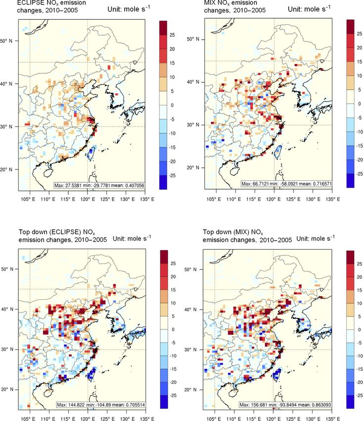
M. Li et al.: Comparison and evaluation of anthropogenic emissions of SO2 and NOx over China                                 3435

ing to emission discrepancies is provided in Sect. 3.3. Finally,    and aviation to keep source consistency in comparison to
Sect. 4 gives the concluding remarks.                               MIX. We developed two sensitivity cases of the ECLIPSE
                                                                    emissions by changing the emission estimates or spatial
                                                                    proxies to study the effect of inventory parameterization on
2     Methodology and data                                          model accuracy, as described in Sect. 3.2.1.
                                                                       MIX was developed for 2008 and 2010 (including monthly
2.1    The ECLIPSE and MIX emission inventory                       variation) by combining the up-to-date regional inventories.
                                                                    For China, the monthly MEIC dataset (available at www.
Spatially specific emission inventories of air pollutants           meicmodel.org) and PKU-NH3 (only for NH3 ) inventory are
and greenhouse gases are among key inputs for chemical              used (Li et al., 2017). The MEIC model calculates and up-
transport models (CTMs) and climate models. ECLIPSE                 dates emissions for over 700 anthropogenic sources dynam-
(Klimont et al., 2017) and MIX (Li et al., 2017) emission in-       ically and delivers the dataset online. Activity rates are de-
ventories have been applied in numerous modeling activities         rived from local provincial statistics in China and emission
at global (Stohl et al., 2015) and regional levels, within the      factors are derived from the best available local measure-
ECLIPSE and MICS-Asia (Model Intercomparison Study for              ments and recent peer-reviewed data for China. Power plants
Asia) Phase III projects, respectively. In general, both inven-     are treated as point sources with emissions estimated by fuel
tories use a dynamic technology-based methodology to esti-          type considering actual combustion technology and installed
mate anthropogenic emissions by multiplying activity rates          control measures such as FGD (flue-gas desulfurization); this
with technology-specific emission factors for each source           information is derived from CPED (China coal-fired Power
by administrative unit (province or county) (Klimont et al.,        plant Emissions Database) as described by Liu et al. (2015).
2017; Li et al., 2017). Then, spatial proxies are used to dis-      Following the methodology of Zheng et al. (2014), emissions
tribute emission estimates by province or county to grids to        of the transport sector in MEIC are estimated at the county
satisfy the needs of model simulation. The key features of          level based on comprehensive parameterization of vehicle
both inventories are listed in Table 1.                             ownership, fuel consumption, temporal evolution of emission
   The ECLIPSE dataset is a global emission inventory for           factors and implementation of new environmental standards.
the period of 1990 to 2010 extended by projections to 2050 in       Volatile organic compounds (VOCs) are speciated to more
5-year intervals with monthly variations, developed with the        than 1000 species and lumped to a GEOS-Chem configured
GAINS model (Amann et al., 2011). Primary sources of ac-            mechanism based on source-specific composite profiles and
tivity data are the International Energy Agency (IEA, 2012)         mapping tables in Li et al. (2014).
for fuel use and the UN Food and Agriculture Organization              Monthly gridded emissions of MEIC are generated by ap-
for agriculture (FAO, http://www.fao.org/faostat/en/#home).         plying source-based spatial and temporal profiles (Li et al.,
GAINS distinguishes 172 regions, including provinces for            2017). Provincial emissions of MEIC are firstly distributed to
China, for which regionally specific emission factors and           counties, then further distributed to grids. The former process
technology distributions are assumed.                               was based on statistics by county (i.e., GDP (gross domestic
   Emissions are distributed to grids at a specific resolu-         product), industrial GDP, total population, urban population,
tion (0.5◦ × 0.5◦ for ECLIPSE, longitude × latitude) based          rural population, agricultural activity, vehicle population),
on the percentages of spatial proxies located in grids by           and the latter was based on gridded maps as spatial prox-
source category using GIS (Geographic Information System)           ies (i.e., population density map, road network). For power
techniques. For ECLIPSE, several layers were developed as           plants, locations were determined using Google Earth fol-
spatial proxies in line with those used in the Representa-          lowing the unit-based methodology. Gridded emission prod-
tive Concentration Pathways (RCP) (Lamarque et al., 2010),          ucts of MEIC v1.1 at a resolution of 0.25◦ × 0.25◦ were inte-
i.e., locations of energy and manufacturing facilities, road        grated into MIX. In this work, we updated China’s emissions
networks, shipping routes, human and animal population              with MEIC v1.2 and extended the MIX emissions back to
density, and agricultural land use. Spatial proxies were fur-       2005 following the same methodology.
ther developed within the Global Energy Assessment project
(GEA project; Riahi et al., 2012), including improved popu-         2.2   GEOS-Chem
lation distribution, flaring in oil and gas production, smelters,
and power plants for which provincial emission layers of            GEOS-Chem is an open-access global 3-D CTM widely
MEIC were used. Spatial proxies for both ECLIPSE and                used by about 100 research groups worldwide. The model
MIX are summarized in Table S1 in the Supplement.                   is driven by the GEOS (Goddard Earth Observing Sys-
   In this work, we use a gridded ECLIPSE v5a                       tem) meteorological dataset and includes complete NOx –
dataset (current legislation, CLE; available at http:               Ox –HC–aerosol chemistry (“full chemistry”), covering over
//www.iiasa.ac.at/web/home/research/researchPrograms/               80 species and more than 300 chemical reactions (Bey et al.,
air/ECLIPSEv5a.html) for 2005 and 2010 in China for all             2001; Park et al., 2004).
anthropogenic sources excluding international shipping

www.atmos-chem-phys.net/18/3433/2018/                                                Atmos. Chem. Phys., 18, 3433–3456, 2018
3436                              M. Li et al.: Comparison and evaluation of anthropogenic emissions of SO2 and NOx over China

Table 1. Key features of ECLIPSE v5a and MIX emission inventories.

         Item                                            ECLIPSE v5a                                     MIX
         Year                                            1990–2010 at 5-year intervals                   2005a , 2008, 2010
         Domain                                          Global                                          Asia
         Spatial resolution                              0.5◦ × 0.5◦                                     0.25◦ × 0.25◦
         Temporal resolution                             Monthly                                         Monthly
         Activities included for each sector
         Energy/power                                    Power plants (including combined heat           Power plants (including combined heat and
                                                         and power), energy                              power)
                                                         production–conversion (including district
                                                         heating plants), fossil fuel distribution
         Industry                                        Industrial combustion and processes             Industrial combustion (including industrial
                                                                                                         heating plants) and industrial processes
         Residential                                     Residential combustion sources                  Residential combustion sources (including
                                                                                                         residential heating plants)
         Transportation                                  On-road and off-road transport sourcesb         On-road and off-road transport sourcesb
         Agriculture                                     Livestock and fertilization                     Livestock and fertilization
         Data sources of activity rates
         Power                                           International Energy Agency (IEA)               CPED (Liu et al., 2015)
         Industry                                        International Energy Agency (IEA)               Provincial industrial economy
                                                                                                         statistics (NBS)
         Residential                                     International Energy Agency (IEA)               Provincial energy statistics (NBS)
         Transportation                                  International Energy Agency (IEA)               Provincial energy statistics (NBS);
                                                                                                         Zheng et al. (2014)
         Agriculture                                     UN Food and Agriculture Organizationc           Provincial statistics (NBS,
                                                                                                         Huang et al., 2012)
         Emission factors and technology                 GAINS model (Klimont et al., 2017)              MEIC modeld , process-based model for
                                                                                                         NH3 (Huang et al., 2012)
         Data access                                     http://www.iiasa.ac.at/web/home/                http://www.meicmodel.org/dataset-mix
                                                         research/researchPrograms/air/
                                                         ECLIPSEv5a.html
     a   Developed following the same methodology of Li et al. (2017).
     b   International air and international shipping are not included.
     c   FAO, http://www.fao.org/faostat/en/#home.
     d   Zhang et al. (2009); Lei et al. (2011); Zheng et al. (2014); Liu et al. (2015).

   In this work, the Asian-nested grid GEOS-Chem model                                     2.3   Top-down emission inventory
v9-01-03 driven by GEOS-5 was used to simulate SO2
and the NO2 maps with different emission inventories                                       We developed the top-down emission inventories for SO2
(Chen et al., 2009). Anthropogenic emissions for Asia were                                 and NOx based on the OMI/Aura L2 swath data. For SO2 ,
replaced with MIX and ECLIPSE variants described in                                        we obtained the planetary boundary layer SO2 total verti-
Sect. 3.2.1. The model has a horizontal resolution of 0.667◦ ×                             cal columns from GES DISC (Goddard Earth Sciences Data
0.5◦ (longitude × latitude) covering Asia and 47 vertical lay-                             and Information Services Center) of NASA (Li et al., 2006).
ers. A nonlocal scheme was applied in mixing within the                                    The mass-balance method was used to interpret the top-
planetary boundary layer (Lin and McElroy, 2010). Global                                   down anthropogenic emissions from total columns (Martin
concentrations at 2.5◦ × 2◦ (longitude × latitude) were simu-                              et al., 2003; Lee et al., 2011). For NOx , we used the tropo-
lated to provide time-varying boundary conditions to the tar-                              spheric slant NO2 column data of the DOMINO v2 (Dutch
get region. A 1-month spin-up was conducted to reduce the                                  OMI NO2 version 2) product accessed from the TEMIS web-
effect of initial conditions. To compare with the OMI obser-                               site (Tropospheric Emission Monitoring Internet Service,
vations consistently, we averaged the daily modeled vertical                               http://www.temis.nl/) (Boersma et al., 2011). Slant columns
columns at 13:00–15:00 local time and resampled the model                                  were converted to vertical columns using the air mass factor
on grids that have OMI data.                                                               (AMF), which is sensitive to the NO2 vertical profile (Palmer
                                                                                           et al., 2001; Lamsal et al., 2010). We revised the AMF by re-

Atmos. Chem. Phys., 18, 3433–3456, 2018                                                                     www.atmos-chem-phys.net/18/3433/2018/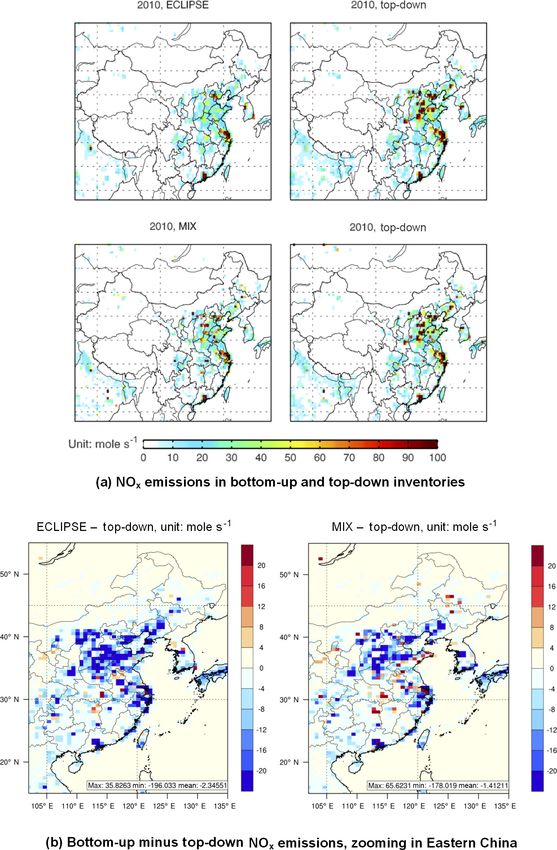
M. Li et al.: Comparison and evaluation of anthropogenic emissions of SO2 and NOx over China                               3437

placing the a priori vertical profiles with the modeled ones      3     Results and discussion
to reduce the bias in comparison following the methodology
of Lamsal et al. (2010). To reduce the retrieval uncertainties,   3.1     Comparisons of ECLIPSE and MIX
we excluded the OMI pixels at a solar zenith angle ≥ 78◦ ,
cloud radiance fraction > 30 %, surface albedo ≥ 0.3 or af-       Following the framework of gridded emission inventory de-
fected by row anomaly (http://projects.knmi.nl/omi/research/      velopment, we conducted parameter-level comparisons be-
product/rowanomaly-background.php). Large pixels near the         tween ECLIPSE and MIX and quantified the reasons caus-
swath edges (10 pixels on each side) are also rejected in spa-    ing the emission differences for each sector. Starting from
tial averaging. Furthermore, daily data of SO2 and NO2 verti-     the emission comparisons for all of China in Sect. 3.1.1, we
cal column density were developed after allocating the OMI        further compared emissions by province in Sect. 3.1.2 and
pixels to model grids (0.667◦ × 0.5◦ ) based on area weights.     gridded emissions in Sect. 3.1.3.
   Top-down NOx emissions were developed following the               As shown in Table 1, the activity rates were assigned inde-
finite difference mass balance (FDMB) methodology (Lam-           pendently by two inventories. As a global emission inventory,
sal et al., 2011; Cooper et al., 2017). We used the sum-          ECLIPSE mainly relies on international statistics of IEA.
mer data to develop the top-down emissions because of             Differently, MIX obtains the official statistics of energy con-
the stronger relationship between local emissions and grid        sumption and industrial output from NBS (National Bureau
columns. The smearing length is around 50 km over China           of Statistics) or MEP (Ministry of Environmental Protec-
in summer (assuming wind speed 5 m s−1 , NO2 lifetime             tion) of China. We can expect high independency for the de-
3 h), comparable to the model grid size, implying weak ef-        termination of emission factors between ECLIPSE (GAINS
fects upon the inversion of horizontal mass transport be-         model) and MIX (MEIC model). As two independently de-
tween grids. Compared to the basic mass-balance method            veloped inventory models, the source classification, technol-
described in Martin et al. (2003), the FDMB method reduces        ogy and removal efficiencies of control facilities in GAINS
the errors from nonlinearity of NOx –OH–O3 chemistry (Gu          and MEIC are expected to be different, although they both re-
et al., 2016; Cooper et al., 2017). A unitless scaling factor β   fer to up-to-date measurements and peer-reviewed data. Dif-
was introduced to represent the sensitivity of fractional mod-    ferent methods were developed in two inventory models for
eled NO2 columns to the fractional anthropogenic emission         specific sectors, including power plants, transportation, and
changes for each grid. We apply 15 % perturbation to emis-        agriculture. For power plants, the spatial proxies were essen-
sions, simulate the NO2 column changes and calculate β fol-       tially consistent between ECLIPSE and MIX. For other sec-
lowing Eq. (1) (Lamsal et al., 2011; Cooper et al., 2017).        tors, emissions were gridded independently by two emission
                                                                  inventories (see Table S1).
1E    1
   =β    ,                                                 (1)
 E                                                               3.1.1    China’s emissions by sectors

where E represents the total NOx emissions and  repre-           Although a comprehensive dataset on fuel consumption and
sents the local NO2 column. 1E is the emission changes of         product yield, surveys on technique penetration and measure-
anthropogenic sources, and 1 is the column changes under         ments of emission factors are incorporated in the inventories,
perturbation.                                                     there are several additional assumptions made to character-
  The top-down emissions were further determined based on         ize some sources for which information is either incomplete
Eq. (2).                                                          or missing. For ECLIPSE and MIX, assumptions are made
                                                                independently and data sources are often different. Particu-
                 t − a                                          larly, MEIC developed high-resolution emissions based on
Et = Ea       1+         β ,                               (2)
                   a                                             unit-based information for the power sector and county-level
                                                                  emissions for transportation.
where Et and Ea represent the top-down and priori emis-              Figure 1 shows the comparisons of China’s emission es-
sions, respectively. t is the OMI-retrieved column. a is        timates in 2005 and 2010 between two inventories for four
the modeled column of GEOS-Chem.                                  key sectors: power, industry, residential and transportation.
   Following Cooper et al. (2017), we limited β within 0.1–       For 2010, ECLIPSE estimates about 28 Tg of SO2 and 22 Tg
10 to avoid biases in regions with negligible low anthro-         of NOx (expressed in Tg NO2 hereafter); 1 and 16 % less
pogenic emissions or columns. The absolute error in the re-       than MIX, respectively. On a sector level, a 40 % difference
trieved NO2 columns is estimated at 1×10¹⁵ molecules cm−2         is found for power plants (higher in ECLIPSE), 24 % for the
(Martin et al., 2003). We filtered out the monthly averaged       industry sector (lower in ECLIPSE) for SO2 , and 15−−21 %
retrieved columns based on this criterion and further devel-      in power and transportation for NOx (lower in ECLIPSE).
oped the top-down emissions for each simulation case. Fi-         It should be noted that heating plants are distributed in the
nally, summer-averaged top-down emissions were developed          power and industry sectors in ECLIPSE, while they are ag-
and applied in the evaluations of this work.                      gregated into industry and residential based on the plant type

www.atmos-chem-phys.net/18/3433/2018/                                              Atmos. Chem. Phys., 18, 3433–3456, 2018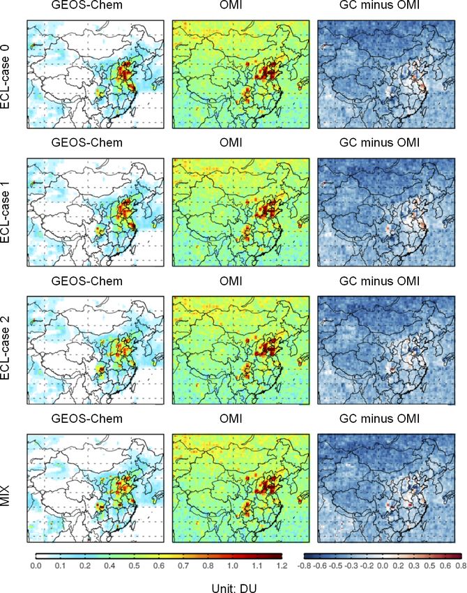
3438                   M. Li et al.: Comparison and evaluation of anthropogenic emissions of SO2 and NOx over China

of fuel combusted in MIX. Redistributing the heating emis-       emission factor, FGD application rate and removal efficiency
sions by aggregating the heating emissions from the industry     all contribute to this discrepancy. SO2 raw emission factor of
and residential sectors to the power sector in MIX will re-      ECLIPSE is 19 % higher than MIX due to different coal qual-
duce the differences to about 11 % (higher in ECLIPSE) in        ity assumed in two inventory models. MIX assumes higher
the power sector and 17 % (lower in ECLIPSE) in industry,        FGD penetration (87.0 % vs. 65.4 %) but lower removal effi-
while increasing the difference in the residential sector from   ciency (80 % vs. 95 %) than ECLIPSE. From 2005 to 2010,
about 10 to 32 % for SO2 and broadening the differences in       the emission discrepancy grew larger because of the decrease
the power sector to around 30 % for NOx (ECLIPSE lower).         in sulfur content and sharply increasing application rates of
   As shown in Fig. 1, emission trends from 2005 to 2010         FGD.
are similar in two inventories, indicating analogous assump-        For NOx , the emission estimates of power plants are simi-
tions of technology evolution driven by economic growth          lar between ECLIPSE and MIX: 7 % difference in 2005 and
and implemented air quality policies in ECLIPSE and MIX.         15 % in 2010. Compared to MIX, the lower emission esti-
In general, MIX estimates larger changes by sectors in the       mates of ECLIPSE are primarily due to emission factors,
analyzed period. Specifically, for power plants, MIX esti-       which are about 20 % lower and can be explained by three
mates a decline for SO2 by 54 %, comparable to the 45 %          factors:
reduction in ECLIPSE, while for NOx both models calculate
about a 10 % increase. MIX estimates slightly larger increas-    (a) Fuel distributions between large and small units. In
ing trends for industrial emissions. For NOx emissions from          MIX, about 89 % of coal was consumed by large or
transport, ECLIPSE calculates lower overall emissions but            medium units (> 100 MW) in 2010, compared to 95 %
higher growth, 26 %, compared to 15 % in MIX.                        in ECLIPSE, reflecting different interpretations of mit-
   The fuel consumptions of MIX and ECLIPSE among dif-               igation strategies during the 11th Five-Year Plan of
ferent sectors in 2010 are presented in Table S2. Owing to           China.
different source structure in each of the models, there are
sometimes significant discrepancies for specific sectors. For    (b) Raw emission factors by technologies. The unabated
example, for coal, the total consumption is relatively con-          emission factor of NOx for existing large power plants
sistent, within 10 % on a mass basis, while in the road trans-       differs within 5 %, while for plants with LNBs (low-
port sector MIX has 28 % higher diesel fuel use. More details        NOx burners), emission factors are 33 % lower in
along with discussion of emissions and implied emission fac-         ECLIPSE. Furthermore, compared to MIX, ECLIPSE
tors are provided below.                                             used 21 % lower emission factors for small plants and
                                                                     26 % lower emission factors for newly built plants.
Coal-fired power plants
                                                                 (c) Application rates of technologies. MIX assumes that in
                                                                     2010 81 % of power plants are equipped with the LNB
For power plants, coal combustion contributes more than
                                                                     techniques while only a 30 % application rate is con-
95 % of SO2 and NOx emissions. Activity rates, assumed
                                                                     sidered in ECLIPSE. The impact of this difference is
heating values, capital sizes, emissions, and key parameters
                                                                     partly offset by higher efficiencies of LNB assumed in
for determining emission factors for coal-fired power plants
                                                                     the latter. Neither model assumed the implementation of
are listed and compared in Table 2.
                                                                     selective catalytic reduction installations in this period.
   The coal consumption of ECLIPSE is 11 − −14 % higher
than MIX in 2005 and 2010 (mass based) due to the differ-
ences in energy statistics and included sources. As a global     Industry
emission inventory model, ECLIPSE (GAINS model) relies
on the energy statistics from IEA (http://www.iea.org/), con-    Comparison of industrial emissions is most challenging since
sistent with the national Energy Balance Sheets provided by      this sector includes a multitude of sources with greatly vary-
the NBS of China (Hong et al., 2017), and also includes dis-     ing emission characteristics and different representation in
trict heating plants. In MIX (MEIC model), coal consump-         the investigated inventories. Overall, ECLIPSE calculates
tion in power plants is derived from CPED, which contains        lower emissions, i.e., 24 and 13 % for SO2 and NOx in 2010
the detailed fuel consumption rates, fuel quality, combustion    and 22 and 0.1 % in 2005, respectively. We compare the pa-
and control technology of over 7600 power-generating units       rameters of the main contributing industrial sources below
in China (Liu et al., 2015). It should be noted that the heat-   keeping the source classification differences in mind.
ing values of coal in China declined between 2005 and 2010,         Coal-fired industrial boilers. MIX estimates about 10.4 Tg
based on the CPED database (Liu et al., 2015).                   of SO2 and 4.3 Tg of NOx emitted from combustion in in-
   ECLIPSE’s SO2 emissions are 37 and 18 % higher than           dustrial boilers, nearly 123 and 71 % more than ECLIPSE.
MIX in 2010 and 2005, respectively. In 2010, the implied         Including fuel use in fuel conversion and the transformation
SO2 emission factor is determined as 6.1 g kg−1 , 24 % higher    sector in ECLIPSE slightly reduces the discrepancy to 101 %
than 4.9 g kg−1 estimated by MIX. As shown in Table 2, raw       for SO2 and 70 % for NOx . While coal consumption of MIX

Atmos. Chem. Phys., 18, 3433–3456, 2018                                           www.atmos-chem-phys.net/18/3433/2018/
M. Li et al.: Comparison and evaluation of anthropogenic emissions of SO2 and NOx over China                              3439

Figure 1. Emissions of SO2 and NOx in 2005 and 2010 by sector over China. NOx emissions are shown in Tg NO2 .

is 29 % larger than ECLIPSE, the key factor contributing to        Residential
the difference is varying emission factors.
   Production of cement and brick. Cement production is            Residential combustion contributes around 10−15 % of SO2
among the major industrial sources, contributing more than         and 6 % of NOx emissions in the considered period. The
26 % of industrial emissions. Both inventories use the same        emission estimates are comparable between two inventories,
cement production rates, while ECLIPSE applies higher              for example for 2010, 4.15 Tg of SO2 and 1.73 Tg of NOx
emission factors leading to 13 and 29 % higher SO2 and             in ECLIPSE and 4.58 Tg of SO2 , 1.38 Tg of NOx in MIX.
NOx emissions than MIX for 2010. For brick production, the         Both models use nearly identical coal consumptions: about
ECLIPSE emission estimates of SO2 and NOx are more than            302 Tg (ECLIPSE) and 306 Tg (MIX), indicating the consis-
3 times higher with a difference in production rate of only        tent statistics from the provincial energy balance table and
25 %. This sector, however, is very uncertain, as information      the national ones for fuel consumed in residential boilers
about fuel use is poorly known and actual emission factors         and/or stoves.
are missing.
   Other sources. One of major reasons for discrepancy is due      Transportation
to oil combustion in the industrial sector where ECLIPSE
assumptions indicate about 36 % lower use than MIX, re-            Transportation sector contributes more than 25 % to the to-
sulting in the 30 % differences for SO2 and NOx emissions.         tal NOx emissions, but is negligible for SO2 emissions.
Another systematic issue is allocation of emissions between        In ECLIPSE, high emitters representing an old and poorly
furnaces and the production process, where for sectors like        maintained vehicle fleet share 12 % of the total transport
pulp and paper, nonferrous metal production, sinter and lime       emissions. ECLIPSE estimates 5.50 Tg of NOx emissions in
production, etc., different approaches are used in the GAINS       2010 (4.86 Tg as shown in Table 3 and 0.64 Tg from high
(ECLIPSE) and MEIC (MIX) models.                                   emitters), 21 % less than MIX. While the ECLIPSE inven-

www.atmos-chem-phys.net/18/3433/2018/                                               Atmos. Chem. Phys., 18, 3433–3456, 2018

3440                            M. Li et al.: Comparison and evaluation of anthropogenic emissions of SO2 and NOx over China

Table 2. Activity rates, emissions and emission factors for SO2 and NOx in power plants of China for 2005 and 2010a .

    Category                      Subcategory                                                              ECLIPSE                            MIX
                                                                                           2005                2010            2005                2010
    Activity rates                Heating value, MJ kg−1                                   20.7                20.7            19.0b               18.8b
                                  Energy consumption, Tg (PJ)                              1202 (24 890)       1743 (36 074)   1055 (20 084)       1577 (29 758)
    Capacity size                 < 100 MW                                                 39.9 %c             5.1 %c          25.0 %              11.5 %
                                  ≥ 100 MW                                                 60.1 %              94.9 %          75.0 %              88.5 %
    SO2 emissions and             SO2 emissions, Gg                                        19 528              10 645          16 516              7754
    emission factors              Average SO2 emission factor, g kg−1                      16.2 (0.79)         6.11 (0.29)     15.6 (0.82)         4.92 (0.26)
                                  (g MJ−1 )
                                  Sulfur content, %                                        1.13                1.13            1.04                0.95
                                  Sulfur retention in ashes, %                             0.092               0.092           0.15                0.15
                                  Raw EFSO2 d , g kg−1                                     22.5                22.5            20.8                19.0
                                  Removal efficiency of FGD, %                             95                  95              80                  80
                                  Application rate of FGD, %                               17.6                65.4            12.6                87.0
    NOx emissions and             NOx emissions, Gg                                        6131                7090            6561                8302
    emission factors              Average NOx emission factor, g kg−1                      5.10 (0.25)         4.07 (0.20)     6.22 (0.33)         5.27 (0.28)
                                  (g MJ−1 )
                                  LNB penetration, %                                       29.4                30.1            53.7                81.4
                                  Unabated EFnox , existing large PP,                      7.55                7.55            7.21                7.21
                                  g kg−1
                                  Unabated EFnox , existing small PP,                      7.04                7.04            8.96                8.96
                                  g kg−1
                                  LNB EFnox , existing large PP, g kg−1                    3.78                3.78            5.63                5.63
                                  LNB EFnox , existing small PP, g kg−1                    3.52                3.52            7.00                7.00
                                  LNB EFnox , newly built PP, g kg−1                       3.11                3.11            4.21                4.21
  a Including both raw coal and derived coal.
  b National average.
  c We interpret the defined small units (< 50 MW) in ECLIPSE to < 100 MW here by assuming that 1/3 of the units in the range of < 100 MW fall into < 50 MW according
  to Liu et al. (2015).
  d The raw EF
                  SO2 is calculated following EF = 2 × sulfur content × (1 − sulfur retention in ashes).

tory includes province-specific fleet characteristics (Klimont                                 hicle types show large differences between ECLIPSE and
et al., 2017), MIX emissions were developed at a county level                                  MIX, indicating the different vehicle fleet assumptions in
by modeling the vehicle stock following the Gompertz func-                                     two inventory models. Detailed data are not known and each
tion, technology distributions in accordance with emission                                     of the inventories (or research groups developing them) re-
standards and emission factors using an international vehicle                                  lied on their own assumptions about fuel consumption per
emission model, as documented by Zheng et al. (2014).                                          vehicle and mileage traveled and combined those with the
   Table 3 compares the fuel consumption, emission esti-                                       available data on the number of vehicles, their sales and re-
mates and net emission factors among various vehicle types                                     tirement rate. Owing to the reasons above, the results can
in two inventories for 2005 and 2010. Parameters for 2005                                      differ significantly. Light-duty vehicles are the largest gaso-
show a similar difference ratio to those in 2010. Assump-                                      line consumer (> 77 %) in both inventories, with 18 % higher
tions for diesel combustion sources (on-road and off-road)                                     gasoline consumption estimated in ECLIPSE than those of
are the main contributor to emission discrepancies. In 2010,                                   MIX in 2010. Accordingly, ECLIPSE estimates less gaso-
diesel emissions of ECLIPSE are over 50 % lower than MIX                                       line consumed in heavy-duty vehicles (74 %) and motorcy-
estimates.                                                                                     cles (32 %) than MIX. These differences reduced from 2005
   Gasoline. There is only a 3 % difference in total gaso-                                     to 2010. Emission estimates of heavy-duty vehicles and mo-
line use in the transport sector between ECLIPSE and MIX.                                      torcycles also show large differences between two inven-
However, emission estimates are significantly different, es-                                   tories. For heavy-duty vehicles, ECLIPSE estimates lower
pecially for light-duty vehicles, which dominate the total.                                    emissions than MIX (66 % in 2010), as a result of less fuel
The consistency in the total gasoline consumption between                                      consumption, while higher emission factors are estimated in
ECLIPSE and MIX is attributed to the consistency in statis-                                    ECLIPSE. For motorcycles, emissions of ECLIPSE are 64 %
tics. As shown in Table 3, the gasoline consumptions by ve-                                    lower than MIX, contributed by both fuel consumption and

Atmos. Chem. Phys., 18, 3433–3456, 2018                                                                              www.atmos-chem-phys.net/18/3433/2018/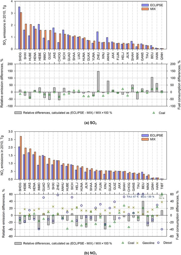
M. Li et al.: Comparison and evaluation of anthropogenic emissions of SO2 and NOx over China                                                                                                   3441

Table 3. Comparisons of activity, emissions and emission factors for the transport sector emission estimates of NOx a .

    Items                         Inventory-year             HDV-G              LDV-G                  MC        All gasoline             HDV-D         LDV-D       All diesel         Diesel
                                                                                                                     on-road                                         on-road         off-road
    Fuel consumptions,            ECL-2005                        3.63              35.0               8.57                47.2              29.7          12.8          42.5            23.1
    Tg                            ECL-2010                        1.50              62.4               7.03                71.0              51.0          20.9          72.0            25.8
                                  MIX-2005                        13.3              25.1               8.30                46.7              59.7          6.11          65.8            35.2
                                  MIX-2010                        5.76              52.8               10.3                68.9              81.2          11.0          92.2            42.1
    NOx emissions,                ECL-2005b                       109                722                 46                878               1570           193          1762           1166
    Gg                            ECL-2010b                        27                582                 34                643               2667           335          3002           1215
                                  MIX-2005                        208                314                129                652               3170           398          3568           1854
                                  MIX-2010                         79                292                 92                463               3614           705          4319           2201
    Average NOx                   ECL-2005c              30.1 (0.70)        20.6 (0.48)        5.4 (0.13)         18.6 (0.43)          52.8 (1.22)   15.1 (0.35)   41.4 (0.96)   50.4 (1.17)
    emission factors,             ECL-2010c              18.0 (0.42)         9.3 (0.22)        4.8 (0.11)          9.1 (0.21)          52.2 (1.21)   16.0 (0.37)   41.7 (0.97)   47.1 (1.09)
    g kg−1 (g MJ−1 )b             MIX-2005               15.6 (0.36)        12.5 (0.29)       15.6 (0.36)         14.0 (0.32)          53.1 (1.23)   65.1 (1.51)   54.2 (1.26)   52.7 (1.22)
                                  MIX-2010               13.7 (0.32)         5.5 (0.13)        9.0 (0.21)          6.7 (0.16)          44.5 (1.03)   64.1 (1.49)   46.8 (1.09)   52.3 (1.21)
   a HDV-G: heavy-/medium-duty buses and trucks – gasoline fueled; LDV-G: light-duty buses, trucks and passenger cars – gasoline fueled; MC: motorcycle; HDV-D: heavy-/medium-duty buses and
   trucks – diesel fueled; LDV-D: light-duty buses and trucks – diesel fueled.
   b High emitters are not included.
   c Emission factors on a mass basis are converted to an energy basis with a heating value of 43.1 MJ kg−1 for gasoline and diesel.

emission factors. It appears that the assumptions about pen-                                                tion of coal use between power and industry since emis-
etration and performance of vehicles with specific emission                                                 sion standards for these sectors are different. MIX estimates
standards vary between the models since the fleet average                                                   lower emissions mainly for eastern China, including Shan-
emission factor in ECLIPSE is 69 % higher than that of MIX,                                                 dong, Hebei, Henan, Jiangsu, Sichuan, Zhejiang and Anhui.
i.e., 9.3 g kg−1 vs. 5.5 g kg−1 .                                                                              For NOx , ECLIPSE estimates are systematically lower
   Diesel. As shown in Table 3, the significant diesel emis-                                                than MIX for most provinces. For 20 provinces, mainly lo-
sion discrepancies can be primarily attributed to the differ-                                               cated in northern and central China, such as Hebei, Shanxi,
ences in fuel consumption. Compared to MIX, ECLIPSE has                                                     Inner Mongolia, Liaoning, Jilin, Heilongjiang and Shandong,
22 % lower diesel use for on-road vehicles and 39 % lower                                                   ECLIPSE emissions are lower by over 20 %. For Beijing,
for off-road engines. While applied emission factors are com-                                               however, ECLIPSE emissions are 41 % higher than MIX
parable for most categories, there is a large discrepancy for                                               driven by a larger estimate for power plants (+36 %) and
light-duty vehicles, where the MIX value is 4 times larger                                                  transport (+114 %). In general, assumptions about diesel
than ECLIPSE. One possible explanation is that there might                                                  consumption in transport vary significantly between inven-
be an issue with assumptions about fuel efficiency that were                                                tories, highlighting the need for further validation of the re-
applied when converting the native MEIC values, which are                                                   gional fuel statistics. It is important to note that, as in many
kilometers driven for activity and gram per kilometer for                                                   other countries, the national and regional energy use statistics
emission factors (Zheng et al., 2014).                                                                      contain limited information about diesel fuel use in trucks
                                                                                                            and non-road engines used in industries in which fuels are
3.1.2     Provincial emission estimates                                                                     allocated to the industry rather than the transport.
                                                                                                               The sectorial distributions of emissions by province are
Provincial emissions were developed using different method-                                                 generally consistent between the two inventories, as pre-
ologies for two inventories (see Sect. 2.1). The provin-                                                    sented in Fig. S1 in the Supplement. For SO2 , the emission
cial emission discrepancies between two inventories are at-                                                 fractions of power plants in MIX are lower, and industrial
tributed primarily to two factors: (i) the differences in ac-                                               fractions are overall higher than those of ECLIPSE due to
tivities, emission factors and policy implementation assump-                                                the differences in source classification and emission factors.
tions at the national level (as discussed in the previous sec-                                              The distribution patterns of NOx provincial emissions show
tion) and (ii) distribution of activities among the provinces –                                             relatively good consistency (within 30 % difference on the
see Sect. 2.1 for principal data sources for the latter.                                                    sector level) between the two inventories.
   Figure 2 compares emissions and the relative difference in
fossil fuel consumption by province in ECLIPSE and MIX in
2010. The differences in provincial SO2 emissions are rela-                                                 3.1.3        Gridded emissions
tively large for a number of provinces, especially when com-
pared to the fluctuations of coal consumption. This indicates                                               Gridded emissions are direct inputs for atmospheric chem-
significant differences in provincial emission factors, which                                               istry models and climate models. We compared ECLIPSE
is mainly because of varying assumptions on application and                                                 and MIX gridded emissions by analyzing three components:
efficiency of abatement measures but also different alloca-                                                 emissions by grids at 0.5◦ × 0.5◦ resolution in 2010, the spa-

www.atmos-chem-phys.net/18/3433/2018/                                                                                                    Atmos. Chem. Phys., 18, 3433–3456, 2018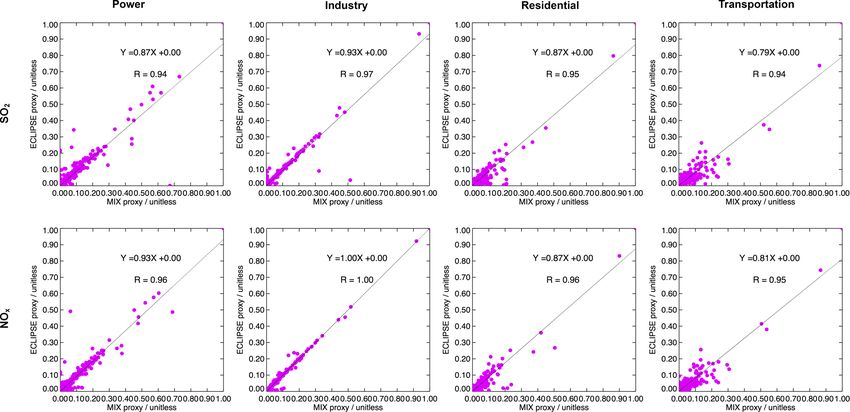
3442                    M. Li et al.: Comparison and evaluation of anthropogenic emissions of SO2 and NOx over China

Figure 2. Comparisons of emission estimates and fuel consumption by province in China in 2010. Values out of y axis range are labeled
separately in the graphs. Abbreviations of provinces are provided in Table S3.

tial proxies used in the gridding process and gridded emis-          ferences discussed earlier. Grids located in eastern parts of
sion trends from 2005 to 2010.                                       China show higher SO2 emissions in ECLIPSE compared
   Gridded emissions. Figure 3 compares the gridded emis-            to MIX. NOx emissions of ECLIPSE are overall lower than
sions between ECLIPSE and MIX for SO2 and NOx . MIX                  MIX, except for Beijing and Guangzhou. Correlations be-
emissions were aggregated from 0.25 to 0.5◦ to be compara-           tween the two gridded emissions are quite good at 0.5◦ ×0.5◦
ble with ECLIPSE. The discrepancies in spatial distribution          grids (slope = 0.83, R = 0.90 for SO2 , slope = 0.79, R =
of gridded emissions are in line with provincial emission dif-       0.98 for NOx ).

Atmos. Chem. Phys., 18, 3433–3456, 2018                                               www.atmos-chem-phys.net/18/3433/2018/
M. Li et al.: Comparison and evaluation of anthropogenic emissions of SO2 and NOx over China                                3443

Figure 3. Comparisons of MIX and ECLIPSE gridded emissions on 0.5◦ × 0.5◦ grids for 2010.

   Sectorial emissions show distinct spatial characteristics       used a two-step allocation method (province to county,
(Fig. 3b). Comparisons of industrial and residential sec-          county to grid). The data sources of spatial proxies also dif-
tors show clear administrative boundaries as these are typi-       fer between the two inventories (see Table S1). We further
cally distributed from provincial emissions using population-      compared the spatial proxies by sector in Fig. 4.
based proxies. Since power plants are treated as point                Spatial proxy. Spatial proxies can play key roles in evalu-
sources, emissions differ in grids over the entire country,        ating the accuracy of emission inventories and CTM simula-
higher for SO2 and lower for NOx in ECLIPSE. Signals of            tion (Geng et al., 2017; Zheng et al., 2017). Proxies used in
large cities are observed in the comparison for the transporta-    the ECLIPSE and MIX emission gridding process are sum-
tion sector because emissions are gridded based on road net-       marized in Sect. 2. Source-specific layers were developed as
work (on-road) or population distribution (off-road).              spatial proxies by ECLIPSE, among which, MEIC emissions
   The differences of gridded emissions illustrated in Fig. 3      were taken to distribute emissions for power plants (Klimont
are attributed to the discrepancies in emission estimates          et al., 2017). For the industry and residential sectors, emis-
nationwide and by provinces (Sect. 3.1.1, 3.1.2) and also          sions are distributed mainly based on population data. Road
method and data of emission spatial allocations (see Sect. 2).     networks and population are used as proxies for transporta-
For power plants that were treated as point sources, emis-         tion emissions. The spatial proxies used in MIX (MEIC) have
sions are gridded based on the locations verified by Google        been summarized in several papers (Geng et al., 2017; Li
Earth (Liu et al., 2015), consistent between ECLIPSE and           et al., 2017), showing that local proxies are used in the grid-
MIX. For other sectors, ECLIPSE gridded the provincial             ding process. MIX (MEIC) uses Google Earth in verifying
emissions according to the source-specific layers, and MEIC        the locations for each power plant. As described in Zheng

www.atmos-chem-phys.net/18/3433/2018/                                               Atmos. Chem. Phys., 18, 3433–3456, 2018
3444                      M. Li et al.: Comparison and evaluation of anthropogenic emissions of SO2 and NOx over China

Figure 4. Emission distribution ratios within provinces in China in 2010 at 0.5◦ × 0.5◦ resolution.

et al. (2014), for the transport sector, the China digital road-            In MIX, decreasing emissions for the Beijing and PRD
network map is used for emission distribution. Other prox-               (Pearl River Delta) regions are estimated, which are domi-
ies including the total population map (for some industrial              nated by a decline in the power and transport sectors, in con-
sources), urban population map (for industrial heating, resi-            trast to the increasing emission trend of ECLIPSE. The dif-
dential coal burning, etc.) and rural population map (for res-           ferent trends of transportation emissions are attributed to the
idential biofuel burning) are in general consistent with the             different assumptions about the legislation effect on pollution
global inventory (Geng et al., 2017).                                    control in the two inventory systems. For Beijing, the differ-
   In this work, we calculated the distribution ratios, reflect-         ences in the transportation emission trend are mainly caused
ing the spatial proxies used, by dividing the emissions for              by diesel vehicles. In ECLIPSE, 47 % increases are estimated
each grid by the provincial emissions for each sector. The               for diesel-fueled vehicles, compared to 28 % emission de-
distribution ratios between ECLIPSE and MIX in 2010 are                  creases in MIX. Fuel consumptions show large discrepancies
shown in Fig. 4. Good correlations (slope ≥ 0.79, R ≥ 0.94)              in the trend from 2005 to 2010, with +54 % (ECLIPSE) com-
are observed for all sectors, which is reasonable because sim-           pared to −20 % (MIX) for heavy-duty vehicles and +45 %
ilar proxy datasets were used in the two inventories, as illus-          (ECLIPSE) compared to +3 % (MIX) for light-duty vehi-
trated above. The differences for specific sectors (e.g., res-           cles. The emission factors of light-duty vehicles increase by
idential with a slope of 0.87, transportation with a slope of            5 % in ECLIPSE, whereas they decrease by 34 % in MIX, at-
0.79–0.81) are higher than others, mainly due to the differ-             tributed to the different assumptions about emission control
ent population datasets and road networks used for emission              effects. As a pioneer in pollution control of China, Beijing
allocation of relevant sources in ECLIPSE and MIX.                       carried out a Euro III standard in 2005 and Euro IV standard
   Emission trend (2005–2010). Fig. 5 presents the emission              in 2008 for light-duty vehicles. The Euro IV penetrations in
changes of SO2 and NOx estimated by ECLIPSE and MIX                      2010 in Beijing are assumed to be around 12 % in ECLIPSE
for the period of 2005 to 2010. For SO2 , the emission trends            and more than 60 % in MIX, which might be too optimistic
are similar between the two inventories: a sharp decrease for            and should be verified with local surveys.
power plants due to the wide application of desulfurization                 For the PRD region, gasoline and heavy-duty diesel vehi-
facilities since 2006 and an overall increase for industrial             cles contribute to the different emission trends. Of the emis-
sources driven by economic growth and still low penetration              sion changes for light-duty gasoline buses, a 22 % increase
of emission control technology, consistent with the national             is estimated in ECLIPSE, compared to 12 % emission reduc-
emission trend analyses in Sect. 3.1.1. For NOx , different              tion in MIX. For heavy-duty diesel vehicles, the trends in fuel
emission trends are estimated for transportation and consis-             consumption (+55 % in ECLIPSE, compared to −11 % in
tent trends are estimated for other sectors.                             MIX) and technology distribution (21 % of Euro III in 2010
                                                                         for ECLIPSE, compared to > 50 % in MIX) are the main

Atmos. Chem. Phys., 18, 3433–3456, 2018                                                    www.atmos-chem-phys.net/18/3433/2018/
M. Li et al.: Comparison and evaluation of anthropogenic emissions of SO2 and NOx over China 3445
Figure 5. SO2 (a) and NOx (b) emission changes from 2005 to 2010 by sectors calculated as E2010 –E2005 , at 0.5◦ × 0.5◦ grids. Note
different color scales are used among sectors.
contributors to the difference. In summary, survey data are tions for NOx emission estimates, spatial proxies and emis-
urgently needed to validate the fuel consumption, effect of sion trends.
legislation and trend for diesel vehicles in pioneering regions
such as Beijing and PRD. 3.2.1 Sensitivity cases for model simulations
The main purpose of this subsection is to evaluate the ef-
3.2 Evaluations from the satellite perspective
fect of gridded emissions on model performance and figure
out the effect of emission estimates and spatial distributions
In this section, we evaluated the effect of emission invento- on model performance using satellite observations as a cri-
ries on the accuracy of model simulations through combing terion. Therefore, we set up four sensitivity cases of mod-
GEOS-Chem Asian-nested modeling and OMI observations eling, ECL-case0, ECL-case1, ECL-case2 and MIX. ECL-
(Sect. 3.2.1). Top-down emissions were developed for both case0 and MIX form the two basic cases, which apply the
SO2 and NOx (Sect. 3.2.2). Due to the large uncertainties ECLIPSE and MIX emissions in the simulation, respectively.
in SO2 retrievals of OMI, we mainly focused on the evalua- ECL-case1 scales China’s emissions in ECLIPSE to MIX’s
www.atmos-chem-phys.net/18/3433/2018/ Atmos. Chem. Phys., 18, 3433–3456, 20183446 M. Li et al.: Comparison and evaluation of anthropogenic emissions of SO2 and NOx over China
value by sectors retaining original spatial distributions. ECL- can be concluded that ECLIPSE and MIX are consistent
case2 redistributes the ECLIPSE emissions over China based with the top-down estimates over China. Summer-averaged
on the spatial grid ratios of MIX, also on the sector level. bottom-up emissions show strong correlations with the top-
The characteristics of the emission inventory used for each down ones (R > 0.87 for both inventories) in 2010. The
case are summarized in Table 4 and shown in Fig. S2. We mean biases of MIX are −21.2 % (11.9 mol s−1 in RMSE),
processed each inventory into model-ready inputs through much lower than −39.4 % of ECLIPSE (14.6 mol s−1 in
regridding new emissions, performing VOC speciation and RMSE). The slope ratio of MIX shows a slightly better per-
temporal allocation. The speciation factor and monthly pro- formance than ECLIPSE (0.73 for MIX, 0.50 for ECLIPSE),
files by sector of the MIX inventory are used for ECL-case0– but should be interpreted with caution since the slope can be
case2. We resample the model results based on satellite ob- dominated by several large point sources.
servations spatially and temporally for consistent comparison In spatial distribution, large discrepancies are observed
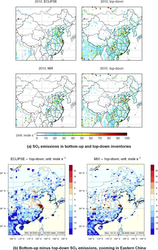
as described in Sect. 2.3. between bottom-up emission inventories and the top-down
Figure 6 compares the SO2 columns simulated by the four ones. For SO2 , bottom-up inventories tend to underesti-
model cases and OMI SO2 columns in 2010. Although OMI mate emissions in Shandong Province and several southern
data tend to overestimate the concentrations due to the over- provinces such as Guizhou, Jiangxi and Fujian, which may
lap in signals of SO2 and O3 during retrieval, good corre- be attributed to the scattered coal consumption, while overes-
lations are found between model results and satellite obser- timating emissions in the Yangtze River Delta (YRD) region
vations (R = 0.633–0.667, slope = 0.842–0.863, generally (see Fig. 8). As shown in Fig. 9, both ECLIPSE and MIX un-
consistent among sensitivity cases; see Table S4), confirm- derestimate the NOx emission strength in northern China and
ing the high accuracies of the priori SO2 spatial emission parts of the YRD and PRD regions and overestimate emis-
patterns. sions located in large cities such as Beijing, Shanghai and
NO2 tropospheric vertical columns modeled for each case Wuhan. One important reason for the latter is associated with
are compared with the retrieved OMI columns (Fig. 7). the limitations of currently used spatial proxies. Using pop-
Summer-averaged results are shown here because of the ulation or industry gross domestic product as a spatial proxy
closer connection between emissions and columns due to may distribute too much emissions to provincial capitals or
short NOx lifetime. As shown in Fig. 7, a modeled NO2 economically developed cities. Through sensitivity test anal-
density map shows a similar spatial pattern among cases, yses, it is concluded that treating sources as point sources can
but different magnitudes. Higher NO2 concentrations are ob- significantly reduce the uncertainties in the emission grid-
served for the ECL-case1 and MIX case because common ding process (Geng et al., 2017).
emission estimates of MIX are used, which are higher than Emission changes from 2005 to 2010 were evaluated and
ECLIPSE. Compared to OMI, all model cases underestimate presented in Fig. 10 for SO2 and Fig. 11 for NOx . The
the pollution in northern China and slightly overestimate the maps of SO2 emission changes are consistent in spatial pat-
columns over central China. As illustrated in Table 4, the per- terns between bottom-up and top-down inventories. Effec-
formance of the MIX case is the best among all cases, identi- tive control measures including nationwide FGD application
fied by low biases (NMB = −4.72 %) and a better slope ratio led to a significant SO2 emission decrease between 2005
(slope = 0.601). The results of ECL-case0 and ECL-case2 and 2010, especially in Beijing, Hebei, Shanxi, YRD, PRD
are similar because the differences in spatial proxies of two and the southwest provinces of China. The annual growth
inventories are small compared to the differences in emission rate of China’s emissions of NOx is highly consistently es-
estimates (Sect. 3.1.3). Replacing the emission estimates of timated by ECLIPSE, MIX and satellite-based inventories,
ECLIPSE with MIX improves the model performance from around 4.0 % annual growth in the period of 2005 to 2010
bias at −12.2 to −6.19 % (ECL-case1 vs. ECL-case0). (see Table 5). The results are comparable with previous work
using various inversion methodologies, satellite sensors or
3.2.2 Top-down emission evaluations CTMs (Gu et al., 2013; Krotkov et al., 2016; Miyazaki et al.,
2017). Figure 11 shows the gridded emission changes from
Satellite-based emission inventories were developed follow- 2005 to 2010 among different inventories for NOx . A de-
ing the finite difference mass balance methodology (Cooper crease in parts of the YRD and PRD regions and shut down
et al., 2017). Emissions of SO2 estimated by bottom-up of large facilities are captured by satellite, showing gener-
and top-down inventories are presented in Table S5. Both ally consistency with MIX. Significantly larger growth is ob-
ECLIPSE and MIX correlate well with the top-down esti- served in northern China’s emissions from top-down inven-
mates (R = 0.722–0.896, slope = 0.539–0.923) in 2005 and tories than in estimates of ECLIPSE and MIX. In Beijing, the
2010. Relatively high negative biases are found (NMB = satellite-based inventory shows a relatively stable trend, dif-
−51.0 ∼ −29.1 %) in the bottom-up inventories, possibly at- ferent from the increasing trend of ECLIPSE or decreasing
tributed to the uncertainties in the OMI retrievals for SO2 . trend of MIX, indicating that assumptions about the penetra-
Table 5 shows the NOx emission estimates and correlations tion of emission reduction technology need further revision
between bottom-up and top-down inventories. For NOx , it in both inventory models for large cities.
Atmos. Chem. Phys., 18, 3433–3456, 2018 www.atmos-chem-phys.net/18/3433/2018/You can also read