A study of the dynamical characteristics of inertia-gravity waves in the Antarctic mesosphere combining the PANSY radar and a non-hydrostatic ...
←
→
Page content transcription
If your browser does not render page correctly, please read the page content below
Atmos. Chem. Phys., 19, 3395–3415, 2019
https://doi.org/10.5194/acp-19-3395-2019
© Author(s) 2019. This work is distributed under
the Creative Commons Attribution 4.0 License.

A study of the dynamical characteristics of inertia–gravity waves in
the Antarctic mesosphere combining the PANSY radar and a
non-hydrostatic general circulation model
Ryosuke Shibuya1 and Kaoru Sato2
1 Japan   Agency for Marine-Earth Science and Technology, Yokohama, Japan
2 Department   of Earth and Planetary Science, The University of Tokyo, Tokyo, Japan

Correspondence: Ryosuke Shibuya (shibuyar@jamstec.go.jp)

Received: 27 September 2018 – Discussion started: 17 October 2018
Revised: 15 January 2019 – Accepted: 8 March 2019 – Published: 18 March 2019

Abstract. This study aims to examine the dynamical char-            originates from 75◦ S due to topographic gravity waves gen-
acteristics of gravity waves with relatively low frequency          erated over the Antarctic Peninsula and its coast, while more
in the Antarctic mesosphere via the first long-term simula-         than 80 % of the other branch originates from 45◦ S and in-
tion using a high-top high-resolution non-hydrostatic general       cludes contributions by non-orographic gravity waves. The
circulation model (NICAM). Successive runs lasting 7 days           existence of isolated peaks in the high-latitude region in the
are performed using initial conditions from the MERRA re-           mesosphere is likely explained by the poleward propagation
analysis data with an overlap of 2 days between consecu-            of quasi-inertia–gravity waves and by the accumulation of
tive runs in the period from April to August in 2016. The           wave energies near the inertial frequency at each latitude.
data for the analyses were compiled from the last 5 days of
each run. The simulated wind fields were closely compared
to the MERRA reanalysis data and to the observational data
collected by a complete PANSY (Program of the Antarctic             1   Introduction
Syowa MST/IS radar) radar system installed at Syowa Sta-
tion (39.6◦ E, 69.0◦ S). It is shown that the NICAM meso-           Waves propagating in the stably stratified atmosphere with
spheric wind fields are realistic, even though the amplitudes       buoyancy as a restoring force are traditionally called gravity
of the wind disturbances appear to be larger than those from        waves. Gravity waves transport momentum upward from the
the radar observations.                                             troposphere to the middle atmosphere and are recognized as
   The power spectrum of the meridional wind fluctuations           a major driving force for large-scale meridional circulation in
at a height of 70 km has an isolated and broad peak at fre-         the middle atmosphere (e.g., Fritts and Alexander, 2003). Be-
quencies slightly lower than the inertial frequency, f , for lat-   cause the horizontal wavelengths of significant parts of grav-
itudes from 30 to 75◦ S, while another isolated peak is ob-         ity waves are shorter than several hundreds of kilometers,
served at frequencies of approximately 2π/8 h at latitudes          many climate models use parameterization methods to cal-
from 78 to 90◦ S. The spectrum of the vertical fluxes of the        culate momentum deposition via unresolved gravity waves
zonal momentum also has an isolated peak at frequencies             (e.g., McFarlane, 1987; Scinocca, 2003; Richter et al., 2010).
slightly lower than f at latitudes from 30 to 75◦ S at a height     Currently, many gravity wave parameterizations are based on
of 70 km. It is shown that these isolated peaks are primarily       very simple assumptions related to essential wave dynam-
composed of gravity waves with horizontal wavelengths of            ics, such as source spectra and propagation properties. Even
more than 1000 km. The latitude–height structure of the mo-         though physically based gravity wave parameterizations have
mentum fluxes indicates that the isolated peaks at frequen-         recently been developed (e.g., Beres et al., 2004; Song and
cies slightly lower than f originate from two branches of           Chun, 2005; Cámara et al., 2014; Charron and Manzini,
gravity wave propagation paths. It is thought that one branch       2002; Richter et al., 2010), tuning parameters, which are

Published by Copernicus Publications on behalf of the European Geosciences Union.
3396                             R. Shibuya and K. Sato: A study of the dynamical characteristics of inertia–gravity waves

ill-defined in general circulation models, such as the mov-          frequency spectrum analyses of the horizontal winds (e.g.,
ing speeds of sub-grid convective cells related to the phase         Kovalam and Vincent, 2003) or from variance analyses of
speeds of launched gravity waves (Beres et al., 2004; Choi           gravity wave wind fluctuations and their seasonal (e.g., Hi-
and Chun, 2011) or the occurrence rate for wave launching            bbins et al., 2007) and interannual (e.g., Yasui et al., 2016)
for the frontogenesis function (Richter et al., 2010), still ex-     variations. Even though a few studies using ground-based ob-
ist.                                                                 servations attempted to estimate the sources of the observed
   Geller et al. (2013) showed that parameterized gravity            mesospheric gravity waves using heuristic ray tracing meth-
waves in climate models are not realistic in several aspects,        ods (e.g., Nicolls et al., 2010; Chen et al., 2013), a statistical
particularly at high latitude, compared to high-resolution ob-       analysis is required to understand the dynamical characteris-
servations and high-resolution general circulation models.           tics of mesospheric gravity waves.
Such improper specifications of gravity wave momentum                    Observational instruments on board satellites have also
deposition by parameterizations are thought to lead to sev-          been used to detect the spatial distributions of temperature
eral serious problems, such as the so-called cold-pole bias          (radiance) data in the mesosphere (MLS: Wu and Waters,
problem (SPARC, 2010; McLandress et al., 2012; Garcia et             1996; Jiang et al., 2005; CRISTA: Preusse et al., 2006;
al., 2017). However, many previous studies have suggested            SABER: Preusse et al., 2009; Yamashita et al., 2013). In
that the Antarctic region has multiple types of gravity wave         addition, the momentum flux of mesospheric gravity waves
sources, such as the mountains of the southern Andes and             is estimated using the SABER temperature data (Ern et al.,
the Antarctic Peninsula (e.g., Eckermann and Preusse, 1999;          2018). However, the variances and momentum fluxes esti-
Alexander and Teitelbaum, 2007; Sato et al., 2012), the small        mated from satellite data contain contributions from a limited
islands around the Southern Ocean (Wu et al., 2006; Alexan-          portion of the gravity wave spectrum due to the observational
der et al., 2010; Hoffmann et al., 2013), the leeward propaga-       filtering effects of each satellite instrument (e.g., Alexander
tion of gravity waves from lower and high latitudes (Sato et         et al., 2010).
al., 2009, 2012; Hindley et al., 2015), the upper tropospheric           To examine the dynamical characteristics of gravity
jet stream (Shibuya et al., 2015; Jewtoukoff et al., 2015), and      waves, high-resolution general circulation models that di-
the strong polar night jet (Yoshiki and Sato, 2000; Sato and         rectly resolve a relatively wide range of the gravity wave
Yoshiki, 2008; Sato et al., 2012). Therefore, these processes        spectrum are powerful tools. At present, however, only four
may frequently overlap in time and space, suggesting that            models have been used to directly resolve mesospheric grav-
process-based analyses based on observational data are un-           ity waves with minimal resolved horizontal wavelengths
avoidable. In response to such recognitions of the importance        (λmin ) of less than 400 km and with fine vertical resolu-
of gravity waves in the Antarctic, several observational cam-        tions (dz) of less than 600 m in the middle atmosphere.
paigns in the lower stratosphere have been conducted (e.g.,          Becker (2009) used the Kühlungsborn Mechanistic Gen-
VORCORE, Hertzog et al., 2008; CONCORDIASI, Rabier                   eral Circulation Model (KMCM) to examine the sensitiv-
et al., 2010; DEEPWAVE, Fritts et al., 2016).                        ity of the state of the upper mesosphere to the strength of
   Due to the harsh environment in the Antarctic, it is still        the Lorenz energy cycle in the troposphere. Zülicke and
challenging to perform observation of the mesosphere. Pre-           Becker (2013) used KMCM to examine the dynamical re-
vious studies have used several observational instruments            sponses of the mesosphere to a stratospheric sudden warm-
at limited ground-based observation sites, such as medium-           ing (SSW) event. In addition, by combining KMCM sim-
frequency (MF) radar (e.g., Dowdy et al., 2007), meteor radar        ulations and MF radar observations in the Northern Hemi-
(Tsutsumi et al., 1994; Forbes et al., 1995), metal fluores-         sphere, Hoffman et al. (2010) explored the relationship be-
cence lidar (e.g., Gardner et al., 1993; Arnold and She, 2003;       tween the activities of mesospheric gravity waves and crit-
Chen et al., 2016), and airglow imagers (e.g., Garcia et al.,        ical level filtering via background wind. Liu et al. (2014)
2000; Matsuda et al., 2014). Using these instruments, these          used the mesosphere-resolving version of the Whole At-
studies have primarily focused on the temporal–spatial struc-        mosphere Community Climate Model to create a horizontal
tures of migrating and non-migrating tides using observa-            map of mesospheric perturbations such as concentric grav-
tional data at one or a couple Antarctic stations (e.g., Mur-        ity waves, which are likely excited by deep convection in
phy et al., 2006, 2009; Hibbins et al., 2010) and the gener-         the low to middle latitudes. The KANTO model (Watanabe
ation and propagation mechanisms of tides using numerical            et al., 2008) is based on the atmospheric component of ver-
models (e.g., Aso, 2007; Talaat and Mayr, 2011). However,            sion 3.2 of the Model for Interdisciplinary Research on Cli-
the dominant vertical wavenumbers of gravity waves have              mate (MIROC; K-1 Model Developers, 2004; Nozawa et al.,
rarely been examined due to the coarse vertical resolution           2007). Sato et al. (2009) used KANTO to discuss the dom-
of the MF radars. Moreover, due to the limited number of             inant sources of mesospheric gravity waves using character-
Antarctic stations, it is still very difficult to examine the spa-   istics of the 3-D momentum flux distribution. Tomikawa et
tial structures of gravity waves observed in the mesosphere.         al. (2012) examined the dynamical mechanism of an ele-
Therefore, discussions concerning the dynamics of gravity            vated stratopause event associated with an SSW event that
waves in previous studies have been based on results from            spontaneously occurred in the KANTO model. Last, the

Atmos. Chem. Phys., 19, 3395–3415, 2019                                                www.atmos-chem-phys.net/19/3395/2019/
R. Shibuya and K. Sato: A study of the dynamical characteristics of inertia–gravity waves                                   3397

JAGUAR model is the KANTO model with the model top ex-            ulated wind fields are closely compared to the PANSY radar
tended to ztop ∼= 150 km including nonlocal thermodynamic         observations at small scales and the MERRA reanalysis data
equilibrium (non-LTE) for infrared radiation processes. Us-       at large scales. In addition, the statistical characteristics of
ing JAGUAR, Watanabe and Miyahara (2009) examined the             the mesospheric disturbances simulated by NICAM, such as
dynamical relationship between migrating tides and gravity        the frequency (ω) spectra of each variable, the kinetic and
wave forcing at low latitudes. Note that all the current models   potential energies, and the momentum and energy fluxes of
permitting mesospheric gravity waves described above are          the gravity waves, are examined.
hydrostatic general circulation models.                              This paper is organized as follows. The methodology is de-
   As mentioned above, a few studies have focused on the dy-      scribed in Sect. 2. The numerical results are compared to the
namical characteristics of gravity waves, such as their prop-     observational results in Sect. 3. The gravity wave character-
agation and/or generation processes in the Antarctic meso-        istics are examined based on a spectrum analysis in Sect. 4.
sphere. However, no study has attempted to simulate meso-         A discussion is presented in Sect. 5, and Sect. 6 summarizes
spheric gravity waves whose reality is confirmed via high-        the results and provides concluding remarks.
resolution observations for a long time period. This is par-
tially because there are few observational instruments with
a sufficiently high resolution to validate mesospheric gravity    2     Methodology
waves simulated in models. Therefore, the dynamical char-
                                                                  2.1    The PANSY radar observations
acteristics of gravity waves observed in the Antarctic meso-
sphere have not been fully examined using both observations       The PANSY radar is the first MST/IS radar in the Antarc-
and numerical simulations.                                        tic and is installed at Syowa Station (39.6◦ E, 69.0◦ S) to
   This study uses two novel methods. One is the first            observe the Antarctic atmosphere in the height range from
Mesosphere–Stratosphere–Troposphere/Incoherent Scatter-           1.5 to 500 km. Note that an observational gap exists from
ing (MST/IS) radar in the Antarctic, which was recently in-       25 to 60 km due to the lack of backscatter echoes in this
stalled at Syowa Station (39.6◦ E, 69.0◦ S) by the “Program       height region (Sato et al., 2014). The PANSY radar employs
of the Antarctic Syowa MST/IS radar” project (the PANSY           a pulse-modulated monostatic Doppler radar system with an
radar; Sato et al., 2014). The PANSY radar is capable of cap-     active phased array consisting of 1045 crossed-Yagi anten-
turing the fine vertical structures of horizontal and vertical    nas. The PANSY radar observations of the 3-D winds have
mesospheric wind disturbances when the mesosphere is ion-         standard time and height resolutions along the beam direction
ized, primarily by solar radiation during the daytime. Such       of 1t =∼ 1 min and 1z = 150 m for the troposphere and
a high resolution is unique in the Antarctic. This means that     lower stratosphere and 1t =∼ 1 min and 1z = 300–600 m
the observational data from the PANSY radar can be used to        for the mesosphere. The accuracy of the line-of-sight wind
validate the results of models permitting mesospheric grav-       velocity is approximately 0.1 m s−1 . Because the target of
ity waves at fine vertical resolution. Furthermore, this study    the MST radars is the atmospheric turbulence, wind measure-
uses the high-top version (Shibuya et al., 2017) of the Non-      ments can be made under all weather conditions. Continuous
hydrostatic Icosahedral Atmospheric Model (NICAM; Satoh           observations have been made by a partial PANSY radar sys-
et al., 2014). This is a global cloud-resolving model with a      tem since 30 April 2012 and by a full system since October
non-hydrostatic dynamical core with icosahedral grids. Such       2015. See Sato et al. (2014) for further details concerning the
a non-hydrostatic model is likely preferable for simulations      PANSY radar system.
of the high-intrinsic-frequency gravity waves contributing            The PANSY radar data that we use are line-of-sight wind
to a large portion of the momentum flux convergence in            velocities of five vertical beams in the vertical direction and
the upper-middle atmosphere (e.g., Reid and Vincent, 1987;        tilted east, west, north, and south at a zenith angle of θ = 10◦
Fritts and Vincent, 1987; Fritts, 2000; Sato et al., 2017).       for the period of April–May 2016, during which the PANSY
Moreover, gravity waves generated by deep convection are          radar frequently detects the PMWEs at heights of 60–80 km
expected to be correctly resolved in non-hydrostatic models.      (Nishiyama et al., 2015). The vertical wind component is
   Recently, using continuous PANSY radar observations            directly estimated from the vertical beam. The zonal wind
of polar mesosphere summer echoes (PMWEs) at heights              component is obtained using a pair of line-of-sight velocities
from 81 to 93 km, Sato et al. (2017) showed that relatively       from the east and west beams. The line-of-sight velocities
low-frequency disturbances from 1 day−1 to 1 h−1 primar-          of the east and west beams, V±θ , are composed of the zonal
ily contribute to the zonal and meridional momentum fluxes.       and vertical components of the wind velocity (u±θ , w±θ ) in
This study examines the dynamical characteristics of gravity      a targeted volume range:
waves with relatively low frequency in the Antarctic meso-
sphere, such as the wave parameters, propagation, and gen-        V±θ = ±u±θ sin θ + w±θ cos θ.
eration mechanisms, via a long-term simulation using the
high-top high-resolution non-hydrostatic general circulation      Assuming that the wind field is homogeneous at each height,
model for 5 months from April to August in 2016. The sim-         i.e., u+θ = u−θ ≡ u and w+θ = w−θ ≡ w, we can estimate

www.atmos-chem-phys.net/19/3395/2019/                                              Atmos. Chem. Phys., 19, 3395–3415, 2019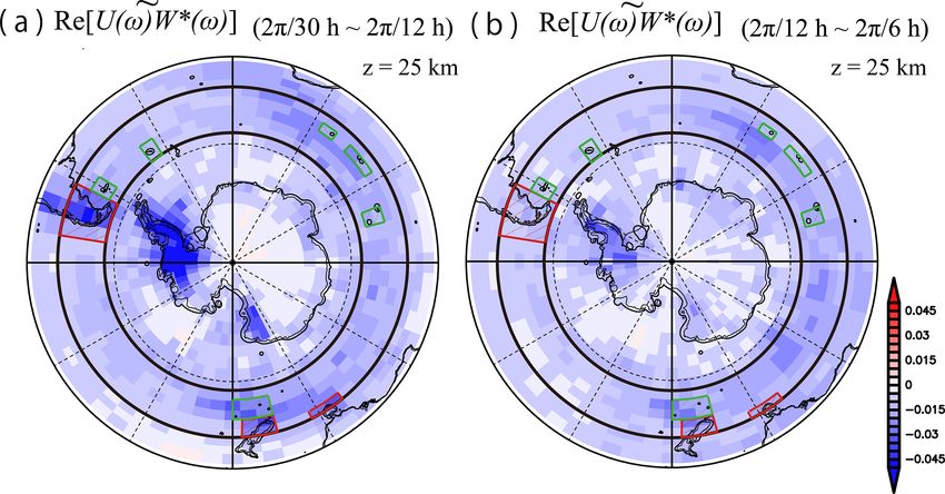
3398                             R. Shibuya and K. Sato: A study of the dynamical characteristics of inertia–gravity waves

the zonal wind component as                                          that little wave reflection near the sponge layer occurs under
                                                                     this setting (not shown). In addition, to prevent numerical
      V+θ − V−θ                                                      instabilities in the model domain, sixth-order Laplacian hor-
u=              .
        2 sin θ                                                      izontal hyperviscosity diffusion is used over the entire height
The meridional wind component is estimated in the same               region. The e-folding time of the ∇ 6 horizontal diffusion for
way using the north and south beams.                                 a 21x wave at the top of the model is approximately 2 s.
                                                                     As a result, the high-top NICAM model can resolve grav-
2.2     Numerical setup for the non-hydrostatic model                ity waves with horizontal wavelengths longer than approx-
        simulation                                                   imately 250 km. Table 1 summarizes the physical schemes
                                                                     used in this study. No cumulus or gravity wave parameteriza-
The simulation was performed using the NICAM, which is               tions were employed. Note that this model does not use the
a global cloud-resolving model (Satoh et al., 2008, 2014).           nudging method as an external forcing for the atmospheric
The non-hydrostatic dynamical core of the NICAM was de-              component.
veloped using icosahedral grids modified via the spring dy-
namics method (Tomita et al., 2002). The simulation period           2.2.2   Initial condition and time integration technique
is from 20 March to 31 August 2016.
                                                                     MERRA reanalysis data based on the Goddard Earth Ob-
2.2.1    Grid coordinate system and physical schemes                 serving System Data Analysis System, Version 5 (GEOS-5
                                                                     DAS; Rienecker et al., 2011) is used as the initial condition
The resolution of the horizontal icosahedral grids is repre-         for the atmosphere. The initial data for the land surface and
sented by g-level n (grid-division-level n). G-level 0 denotes       slab ocean models were interpolated from the 1.0◦ gridded
the original icosahedron. By recursively dividing each trian-        National Centers for Environmental Prediction final analysis.
gle into four smaller triangles, a higher resolution is obtained.    In the MERRA reanalysis data, the following two types of 3-
The total number of grid points is Ng = 10·4n +2 for g-level         D fields are provided: one is produced using the corrector
n. The actual resolution corresponds to q the square root of the     segment of the incremental analysis update (IAU; Bloom et
averaged control volume area, 1x ≡ 4π RE2 /Ng , where RE             al., 1996) cycle (1.25◦ × 1.25◦ with 42 vertical levels whose
is the Earth’s radius. A grid with g-level 8 is used in this study   top is 0.1 hPa) and the other pertains to fields resulting from
(1x ∼ 28 km).                                                        the grid point statistical interpolation analyses (GSI analy-
   Recently, Shibuya et al. (2016) developed a new icosahe-          sis; e.g., Wu et al., 2002) on a native horizontal grid with
dral grid configuration that has a quasi-uniform and region-         native model vertical levels (0.75◦ × 0.75◦ with 72 vertical
ally fine mesh within a circular region using spring dynamics.       levels whose top is 0.01 hPa). We use the former 3-D as-
This method clusters grid points over a sphere into a circular       similated fields from 1000 to 0.1 hPa and the latter 3-D an-
region (the target region). By introducing sets of mathemat-         alyzed fields from 0.1 to 0.01 hPa for the initial conditions
ical constraints, it has been shown that the minimum resolu-         of the NICAM simulation to prepare realistic atmospheric
tion within the target region is uniquely determined by the          fields in the mesosphere. The latter 3-D analyzed fields were
area of the target region. In this study, the target region for      only used at heights above 0.1 hPa because variables for the
a given g-level is a region south of 30◦ S centered on the           vertical pressure velocity, cloud liquid water, and ice mixing
South Pole, corresponding to a horizontal resolution of ap-          ratios are not included and thus have been set to zero. The
proximately 18 km in the target region.                              vertical pressure velocities, cloud liquid water, and ice mix-
   In order to adequately simulate the structures of the distur-     ing ratios above 0.1 hPa were set to zero. The time step was
bances in the stratosphere and the mesosphere, the vertical          15 s, and the model output was recorded every hour. Note
grid spacing is set to 300 m at heights from 2.4 to 80 km.           that the satellite observation data related to the stratospheric
Note that, according to Watanabe et al. (2015), the gravity          temperature profiles are provided up to 50 km the data assim-
wave momentum flux is not heavily dependent on the ver-              ilation technique is only applied below the height (Sakazaki
tical spacing of the model in the middle atmosphere when             et al., 2012).
1z < 400 m. The number of vertical grids is 288. To prevent             Time integrations were performed following a technique
unphysical wave reflections at the top of the boundary, a 7 km       similar to Plougonven et al. (2013) to maintain long-term
thick sponge layer is set above z = 80 km. Second-order              simulations sufficiently close to the reanalysis data. The time
Laplacian horizontal hyperviscosity diffusion and Rayleigh           integration method is illustrated in Fig. 1. Simulations lasted
damping for the vertical velocity are used in the sponge layer.      7 days for each run with initial conditions from the MERRA
The e-folding time of the ∇ 2 horizontal diffusion for a 21x         reanalysis data with an overlap of 2 days between each run.
wave at the top of the model is 4 s, and the e-folding time          The 2-day overlap consists of the spin-up time for the subse-
of Rayleigh damping for the vertical velocity at the top of          quent simulation. The successive data for the analyses were
the model is 216 s. The diffusivity level gradually increases        compiled using the data from the last 5 days of each run. This
from the bottom to the top of the sponge layer. We confirmed         method allows the model to freely produce gravity waves and

Atmos. Chem. Phys., 19, 3395–3415, 2019                                               www.atmos-chem-phys.net/19/3395/2019/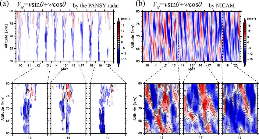
R. Shibuya and K. Sato: A study of the dynamical characteristics of inertia–gravity waves                                                3399

Table 1. Physics scheme used in the high-top NICAM.

                          Physics                  Description
                          Cloud microphysics       NICAM Single-moment Water 6 (NSW6) (Tomita, 2008)
                          Cumulus convection       Not used
                          Radiation                MstrnX (Sekiguchi and Nakajima, 2008)
                          Turbulence               Meller–Yamada Nakanishi–Niino (MYNN2) (Nakanishi and
                                                   Niino, 2006)
                          Gravity wave             Not used
                          Land surface             Minimal Advanced Treatments of Surface Interaction and
                                                   Runoff (MATSIRO) (Takata et al., 2003)
                          Surface flux (ocean)     Bulk surface flux by Louis (1979)
                          Ocean model              Single layer slab ocean

                                                                         At heights of 60–75 km, negative VN values are dominant
                                                                      during the observed periods, which is consistent with the di-
                                                                      rection of the mesospheric residual circulation in the winter
                                                                      hemisphere. On 13 and 16 May it appears that disturbances
                                                                      with negative vertical phase speeds are dominant in the
                                                                      height range of 75–80 km. These features are also observed
                                                                      in the model data in Fig. 2b. The downward-propagating dis-
                                                                      turbances have positive VN values at heights of 75–80 km on
                                                                      13 and 16 May as in Fig. 2a. Therefore, the overall wave
Figure 1. An illustration for the time integration method.            structures are well reproduced by NICAM. However, the
                                                                      phases of the disturbances on 13 May, which is the final day
                                                                      of the 7-day integration from the initial condition, are dif-
mesoscale phenomena without artifacts caused by nudging               ferent from the observations. The possible reason for this is
and assimilation techniques. However, because the succes-             that the propagation path of the wave packet simulated in
sive simulation data are not continuous, spurious and dras-           NICAM on 13 May may be unrealistic since the large-scale
tic jumps in the atmospheric fields between two consecu-              fields likely do not remain sufficiently close to the reanalysis
tive simulations may appear. Therefore, in this study, the sta-       data after such a long simulation time.
tistical analyses are performed by taking an average of the              To quantitatively compare the wave structures observed by
results using the respective 5-day simulations to avoid any           the PANSY radar and those simulated by NICAM, the am-
influences from gaps between the simulations. A long-term             plitudes of the wave disturbances were estimated as a func-
continuous run from a single initial condition was not per-           tion of the vertical phase velocities. Figure 3a and b show
formed because the model fields tend to diverge from the ac-          time–height sections of the line-of-sight winds observed by
tual atmosphere without appropriate parameterization meth-            the north beam of the PANSY radar for 26–28 April and a
ods and/or nudging or assimilation techniques.                        close-up for 28 April 2016, respectively.
                                                                         The estimation method is illustrated below. Here, phase
                                                                      lines at heights of 65–80 km from 04:00 to 18:00 UTC are
3     Results and comparisons of the numerical
                                                                      defined as L1 , L2 , ..., Li , ... LN (denoted by the black lines in
      simulations
                                                                      Fig. 3b) and sets of data points on Li (x1i , x2i , ..., xni i ; the black
3.1    Wave structures in the mesosphere                              circles in Fig. 3b) are defined as Mi (x1i , x2i , ..., xni i ∈ Mi ).
                                                                      The estimated amplitude A of disturbances with the vertical
Figure 2 shows time–height sections of the line-of-sight              phase velocity V1 is defined by calculating the average of the
winds observed by the north beam of the PANSY radar and               covariances of M1 , M2 , . . .MN :
VN calculated using v and w simulated by NICAM for 10–
20 May 2016 (VN = v sin θ + w cos θ , where θ = 10◦ ). The                     X X                  !
missing values in the PANSY radar observation are shown in              2
                                                                      A =2.0 ×      k k
                                                                                   xi xj (i, j ∈ Mk ) /
white. The black dotted vertical lines in Fig. 2b indicate the                         k    i≥j
segments of the continuous 5-day simulations. In the middle                 X X
                                                                                             !
of May, large amounts of observational data from the PANSY                     1 (i, j ∈ Mk )                                               (1)
radar are available because strong PMWEs were observed in                     k    i≥j
the daytime during this period.

www.atmos-chem-phys.net/19/3395/2019/                                                      Atmos. Chem. Phys., 19, 3395–3415, 2019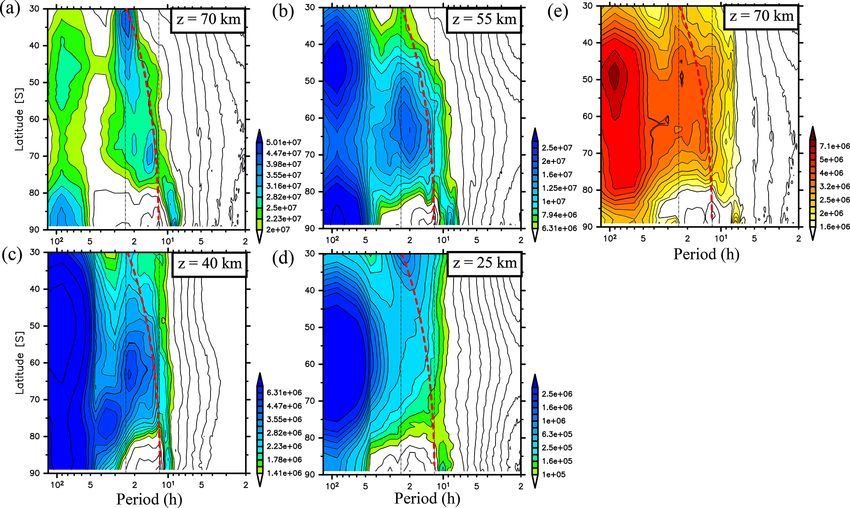
3400                                 R. Shibuya and K. Sato: A study of the dynamical characteristics of inertia–gravity waves

Figure 2. Time–altitude cross sections of northward line-of-sight speeds (a) observed by the PANSY radar at Syowa Station (a) for the
period from 10 to 20 May 2015 and (b) those simulated by NICAM in the same period. The contour intervals are 4 m s−1 . The black dotted
vertical lines in panel (b) denote the segments of the lasting 5-day simulation.

                                                                             estimated amplitude A is equal to the amplitude of the
                                                                             monochromatic wave a. However, the estimated amplitude A
                                                                             becomes very small when phase lines with the vertical phase
                                                                             velocity do not match the wave structure (V2 , the red lines
                                                                             in Fig. 3b). Therefore, the estimated magnitude A has a peak
                                                                             at the dominant vertical phase velocity of the wave distur-
                                                                             bances. In a simple case with cos iπ(2t − z), a result of the
                                                                             estimation by the method is shown as an example in Fig. S1
                                                                             in the Supplement.
                                                                                The main advantage of this method is that it can easily be
                                                                             applied to both simulated data and observed data that have
                                                                             missing values, as in the PANSY radar observations. Prior
                                                                             to the application of this method, a bandpass filter is applied
                                                                             to the observed and simulated northward line-of-sight winds
                                                                             with cutoff wave periods of 2 and 60 h to extract the dominant
                                                                             wave-like structures. In this study, the estimation method for
                                                                             the PANSY radar observation is only applied to data on days
                                                                             for which the ratio of the available data points in a period
                                                                             from 04:00 to 18:00 UTC and at heights of 65–80 km exceeds
                                                                             60 % (25 and 26 April in Fig. 3a). Here, the PANSY radar
                                                                             observation data in April and May are used for this analy-
Figure 3. Time–altitude cross sections of northward line-of-sight            sis since large numbers of observational data are available in
speeds (a) observed by the PANSY radar for the period from (a) 24            these months (12 and 16 days, respectively).
to 26 April 2016 and (b) 26 April 2016. (b) Phase lines with a verti-           Figure 4a and b show the estimated amplitude as a function
cal phase velocity of V1 are denoted as L1 , L2 , ..., Li , ..., LN (thick   of the vertical downward phase velocity in April and May us-
black lines), and data points on Li are denoted as x1i , x2i , ..., xni i    ing data from the PANSY radar observations and the NICAM
(black circles). Other phase lines with a vertical phase velocity of
                                                                             simulations, respectively. In Fig. 4a, it appears that the dom-
V2 and data points on their phase lines are depicted by red. Please
see the text in detail.
                                                                             inant wave disturbances observed by the PANSY radar have
                                                                             vertical phase velocities of approximately 0.5 and 0.7 m s−1
                                                                             in April and May, respectively. These features are well sim-
When the disturbance is due to a monochromatic wave de-                      ulated by the NICAM simulations (Fig. 4b). Therefore, the
fined by V1 (ψ = a cos i(mz − ωt), where ω/m = V1 ), the                     dominant wave structures in the time–altitude section in the

Atmos. Chem. Phys., 19, 3395–3415, 2019                                                       www.atmos-chem-phys.net/19/3395/2019/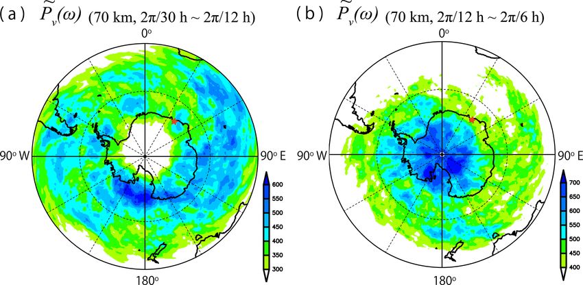
R. Shibuya and K. Sato: A study of the dynamical characteristics of inertia–gravity waves                                        3401

                                                                      simulated by NICAM. In particular, the structure of the po-
                                                                      lar night jet below 35 km in NICAM agrees with that in
                                                                      MERRA. However, the magnitude of the zonal wind around
                                                                      the core of the polar night jet in NICAM is slightly larger
                                                                      than that in MERRA. In addition, the axis of the polar night
                                                                      jet in the mesosphere in NICAM does not tilt as strongly
                                                                      equatorward with height as it does in MERRA. Therefore,
                                                                      the zonal momentum balance in the mesosphere at the initial
                                                                      conditions is not completely maintained in NICAM, likely
                                                                      due to unresolved gravity waves with short horizontal wave-
                                                                      lengths. Even though some discrepancies are observed in the
                                                                      mesosphere, the structure of the polar night jet in NICAM is
Figure 4. Estimated wave amplitude as a function of vertical phase
velocities in April (black curves) and in May (dashed curves) using   sufficiently close to that in MERRA. Hereafter, analyses of
(a) the PANSY radar observation and (b) the NICAM simulation.         the gravity wave characteristics are performed using data for
                                                                      the time period of 1 June–31 August 2016 (JJA).

NICAM simulations are likely very similar to those observed
by the PANSY radar. However, the mesospheric disturbances             4     Gravity wave characteristics in the mesosphere
simulated by NICAM have an approximately 3.5 times larger
                                                                      4.1       Gravity wave energy and momentum fluxes
amplitude than those observed by the PANSY radar. Us-
ing a hodograph analysis, Shibuya et al. (2017) showed that           In this subsection, the spatial structures of the kinetic and po-
NICAM simulations overestimate wave amplitudes by ap-                 tential energies and the momentum and energy fluxes of the
proximately 1.5 times compared to the PANSY radar obser-              gravity waves are examined. The gravity wave component
vations in the mesosphere. The possible reasons for the over-         is defined as wave components with frequencies higher than
estimation of wave amplitude in NICAM will be discussed               2π/30 h. Note that previous studies have defined the plane-
in the end of Sect. 5.                                                tary wave component to have frequencies lower than approx-
                                                                      imately 2π/40 h in the mesosphere (e.g., Murphy et al., 2007;
3.2   Zonal wind components from the troposphere to
                                                                      Baumgaertner et al., 2008).
      the mesosphere
                                                                         In the linear theory of inertia–gravity waves,
Next, zonal wind components simulated by NICAM are
                                                                                    p0 ρ 0 θ 0

compared to those in the MERRA reanalysis data. Figure 5                  u0 , v 0 , w 0 ,
                                                                                       , ,       =
                                                                                    p ρ θ
shows time–altitude cross sections of the zonal winds from
the MERRA reanalysis data and from the NICAM simu-                        u,e
                                                                          e v, w
                                                                               e, p
                                                                                  e, ρ  θ exp i (kx + ly + mz − ωt) ,
                                                                                     e, e                                          (2)
lations for the period of 10–20 May 2016, at a grid near
Syowa Station. In Fig. 5b, jumps between the continuous               where ∼ denotes the Fourier transform of each variable and
5-day simulations are observed in the troposphere and the             ω denotes the ground-based frequency. The polarization re-
lower stratosphere. This is likely because the large-scale            lations for the different variables are written as
flows diverge from the MERRA reanalysis data during the 7-
                                                                             i ω̂k − f l

day integrations. Nevertheless, roughly speaking, the distur-         u=
                                                                      e                    v
                                                                                           e
                                                                             i ω̂l + f k
bances in the troposphere and lower stratosphere are success-               2
                                                                              ω̂ − f 2

fully simulated by NICAM. Conversely, in the upper strato-            p=
                                                                      e                    u
                                                                                           e                                  (3)
sphere and mesosphere, large-amplitude disturbances with                     ω̂k + if l
negative vertical phase speeds are clear in the NICAM data
but rarely seen in the MERRA reanalysis data. Therefore,              and
to validate the dynamical characteristics of the mesospheric                           mω̂
disturbances simulated by NICAM, observational data with              w
                                                                      e=−                     p
                                                                                              e,
                                                                                  N 2 − ω̂2
high vertical and temporal resolution, such as data from the
PANSY radar, are required.                                            where ω̂ denotes the inertial frequency of gravity waves
    In addition, the latitude–altitude structures of the mean         given by
zonal winds averaged in April and May 2016 between the
MERRA reanalysis data and the NICAM simulations are                   ω̂ = ω − U · k.                                              (4)
compared in Fig. 6. In April and May 2016, it appears that
the polar night jet in the upper stratosphere and mesosphere          Using these relations, the real component of the zonal
tilts equatorward with height. Such a feature is successfully         and meridional components of the vertical momentum flux

www.atmos-chem-phys.net/19/3395/2019/                                                         Atmos. Chem. Phys., 19, 3395–3415, 2019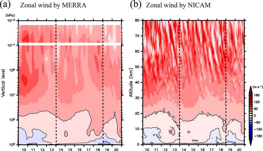
3402 R. Shibuya and K. Sato: A study of the dynamical characteristics of inertia–gravity waves
Figure 5. Time–altitude cross sections of zonal winds (a) from the MERRA reanalysis data and (b) from NICAM simulations for the period
from 10 to 20 May 2015 at a grid near Syowa Station. The contour intervals are 20 m s−1 . The vertical dotted lines denote the segments of
the continuous 5-day simulation by NICAM. (a) The 3-D assimilated fields of the MERRA reanalysis data for 1000 to 0.1 hPa and the 3-D
analyzed fields for 0.1 to 0.01 hPa are drawn.
Because (N 2 − ω̂2 )/(ω̂2 − f 2 ) > 0 and ω̂2 − f 2 > 0 for
inertia–gravity waves, the signs of (u0 w0 , v 0 w0 ) are equal to
those of (k, l) for upward energy propagating waves (i.e.,
m < 0) and the sign of u0 v 0 is equal to that of (k · l). The
horizontal intrinsic group velocities of the gravity wave are
written as
k N 2 − ω̂2 , l N 2 − ω̂2
Ĉgx , Ĉgy = . (6)
ω̂ k 2 + l 2 + m2
Therefore, the directions of the group velocities relative to
the mean wind are also inferred from the signs of the mo-
mentum fluxes. Note that this derivation is based on the as-
sumption of monochromaticity for the inertia–gravity wave.
In addition, the 5-day average in the segment of each simu-
lation is applied in this subsection.
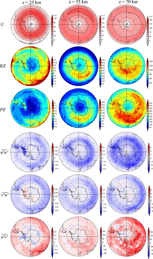
Figure 6. Latitude-altitude cross sections of the zonal mean zonal Figure 7 shows horizontal maps of the zonal wind (U ),
winds (a) from MERRA and (b) from NICAM simulations aver-
the kinetic energy (KE = 12 (u02 + v 02 + w02 )), and the poten-
aged in April and May 2016. The contour intervals are 20 m s−1 . 0 2
2
tial energy (PE = 12 Ng 2 θθ ) divided by the density, u0 w0 ,
v 0 w 0 , and u0 v 0 at heights of 25, 55, and 70 km averaged over
(u0 w0 , v 0 w 0 ) and that of the horizontal momentum flux (u0 v 0 )
JJA. For the estimation of PE, the fluctuation of the potential
are expressed as
temperature is calculated as
N 2 − ω̂2 1 θ0 1 p0
u0 w0 , v 0 w0 = − 2 · (k, l) · w 02 = − ρ 0
, (7)
ω̂ − f 2 m θ ρ0 cs2
and where cs denotes the speed of sound in the atmosphere. The
axis of the polar night jet tilts equatorward with height, as
ω̂2 − f 2 seen in Fig. 6. For KE and PE at a height of 25 km, large
u0 v 0 = kl · · v 02 . (5) energies are distributed near 30◦ S and along the jet axis at
f 2 k 2 + ω̂2 l 2
Atmos. Chem. Phys., 19, 3395–3415, 2019 www.atmos-chem-phys.net/19/3395/2019/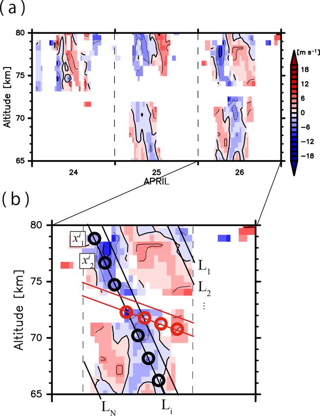
R. Shibuya and K. Sato: A study of the dynamical characteristics of inertia–gravity waves                                                  3403

Figure 7. Horizontal maps of U , KE, PE, u0 w0 , v 0 w0 , and u0 v 0 at heights of 25, 55, and 70 km averaged in JJA. The units of U , KE, and PE
and u0 w0 , v 0 w0 , and u0 v 0 are meters per second, joules per kilogram, and m2 s−2 , respectively.

www.atmos-chem-phys.net/19/3395/2019/                                                         Atmos. Chem. Phys., 19, 3395–3415, 2019
3404 R. Shibuya and K. Sato: A study of the dynamical characteristics of inertia–gravity waves
approximately 60◦ S. Localized energy peaks are also seen in the power spectra estimation, the autocorrelation functions
over the Antarctic Peninsula and the southern Andes and were averaged over JJA. The maximum lag in the calculation
their leeward region, which is consistent with the results of of the autocorrelation function was set to 90 h to increase the
the KANTO model (Sato et al., 2012) and superpressure bal- frequency resolution of the ω spectra; this is 75 % of the sim-
loon and satellite observations. For KE and PE at heights of ulation period (120 h) in each segment.
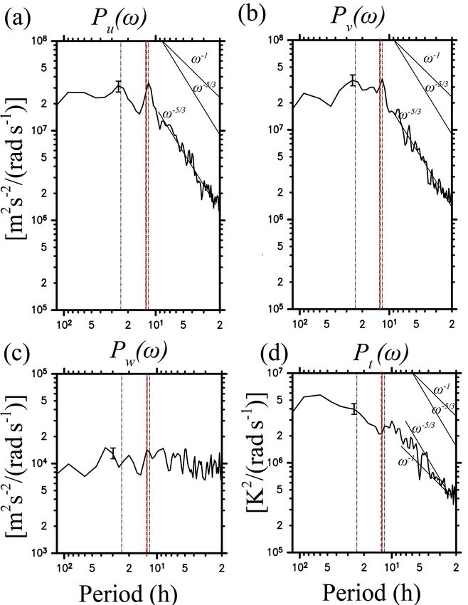
55 and 70 km, large values are observed along latitudinal cir- Figure 8 shows Pu (ω), Pv (ω), Pw (ω), and Pt (ω) for JJA
cles roughly corresponding to the axis of the polar night jet. averaged over heights of 70–75 km at a grid point near Syowa
Strictly speaking, the large values of KE and PE at a height of Station. It is seen that Pu (ω) and Pv (ω) have isolated peaks at
55 km appear to be distributed slightly poleward of the axis a frequency of 2π/12 h, while they obey a power law with an
of the polar night jet, while those of KE at a height of 70 km exponent of approximately −5/3 for frequencies higher than
are broadly distributed but are primarily poleward of 60◦ S. 2π/12 h. Such a power-law structure in the high-frequency
It is interesting that the largest energies are seen near 180◦ E region is consistent with previous observational studies by
at heights of 55 and 70 km. MST radars at midlatitudes (e.g., Muraoka et al., 1990) and
At a height of 25 km, u0 w 0 is primarily negative and large in the Antarctic (Sato et al., 2017). Conversely, Pw (ω) has
values are seen over both the Antarctic Peninsula and the a flat structure (i.e., ∝ ω0 ) for frequencies from 2π/2 h to
southern Andes. Conversely, v 0 w0 is primarily positive over 2π/5 days and has no clear spectral peak. Finally, Pt (ω) does
the Antarctic Peninsula and negative over the southern An- not have a clear peak at the frequency of 2π/12 h but rather a
des. This result suggests the existence of wave-like struc- broad peak at frequencies near 2π/10 h. The spectral slope of
tures with phases aligned in the northwest–southeast direc- Pt (ω) is gentler than −5/3 but steeper than −1 in the high-
tion over the southern Andes and in the northeast–southwest frequency region. Here, the flat spectrum of Pw (ω) can be
direction over the Antarctic Peninsula, which is confirmed by explained by the linear theory of gravity waves. The vertical
previous observational studies (e.g., Alexander and Barnet, velocity is proportional to a buoyancy and temperature:
2007; Hertzog et al., 2008) and by numerical models (e.g.,
Sato et al., 2012; Plougonven et al., 2013). At higher alti- ω̂ 0
w0 = b, (8)
tudes, negative values of u0 w 0 are distributed along the latitu- N2
dinal circle near 60◦ S at a height of 55 km and near 50◦ S at
70 km. Note that the large negative values over the southern where b0 denotes a buoyancy by gravity waves. Conse-
Andes and its leeward region are observed even at a height quently, the variance of w 0 is proportional to ω̂2 b02 . Given
of 70 km. The signs of v 0 w0 are primarily negative along and a buoyancy and temperature spectrum with a frequency ex-
equatorward of the polar night jet axis and positive or weakly ponent between −1 and −5/3, an exponent for the vertical
negative poleward of the jet axis at 25 km. This may indicate frequency spectrum becomes nearly zero, which is consistent
that the gravity waves propagate into the polar night jet as with the result in Fig. 8.
shown in Sato et al. (2009). The sign of u0 v 0 is primarily Next, the zonally averaged v power spectra (Pv (ω)) in JJA
positive at heights of 55 and 70 km, while it is positive equa- without the diurnal and semidiurnal migrating tides and the
torward of 60◦ S and negative poleward of 60◦ S at 25 km. semidiurnal non-migrating tides with s = 1 were calculated
These features are consistent with the distributions of u0 w0 to examine the nontidal low-frequency disturbances (Sato et
and v 0 w0 since the signs of u0 w0 and v 0 w 0 are both negative al., 2017), where s denotes a zonal wavenumber of tides.
(Eq. 5). Therefore, it is suggested that the statistical char- Hereafter, Pv (ω) without these tides is denoted P fv (ω). The
acteristics of disturbances defined as components with wave zonal mean P fv (ω) in JJA is shown as a function of the lati-
frequencies higher than 2π/30 h follow linear relationships tude for the heights of 70, 55, 40, and 25 km in Fig. 9a, b, c,
of the inertia–gravity waves. and d, respectively. The temperature power spectra (P et (ω))
at a height of 70 km are also shown in Fig. 9e. The thick red
4.2 Spectral analysis dashed curves indicate the inertial frequencies at each lati-
tude. Note that the x axis is the ground-based frequency and
4.2.1 The meridional structure of the power spectra not the intrinsic frequency.
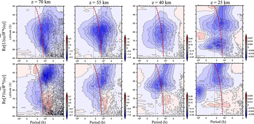
At a height of 70 km, the spectral peaks appear at frequen-
To examine the statistical characteristics of the mesospheric cies slightly lower than the inertial frequencies from 65 to
disturbances simulated by NICAM, the ω power spectra of 75◦ S, as in Fig. 9a. In the midlatitudes, the spectral values
u, v, w, and the temperature (Pu (ω), Pv (ω), Pw (ω), and are maximized near 2π/24 h. Conversely, in regions from 77
Pt (ω), respectively) were obtained for the period of JJA to 90◦ S, the spectral peaks are seen near frequencies from
2016. The power spectra were examined using the Black- 2π/8 to 2π/10 h but are absent at 2π/12 h (and at the in-
man and Tukey (1958) method (e.g., Sato, 1990). First, an ertial frequencies) or 2π/24 h. Such peaks near frequencies
autocorrelation function was calculated for each 5-day sim- from 2π/8 to 2π/10 h in the high-latitude region also appear
ulation to avoid any influences of the gaps between the seg- in Pet (ω) (Fig. 9e). In addition, another branch with frequen-
ments of the simulations. Second, to reduce statistical noise cies smaller than 2π/50 h, which is an order of a frequency of
Atmos. Chem. Phys., 19, 3395–3415, 2019 www.atmos-chem-phys.net/19/3395/2019/R. Shibuya and K. Sato: A study of the dynamical characteristics of inertia–gravity waves 3405
in Fig. 10a, while that at frequencies from 2π/12 to 2π/6 h
is shown in Fig. 10b. It appears that variances for frequen-
cies from 2π/30 to 2π/12 h are broadly distributed around
180◦ E at latitudes poleward of 60◦ S, which is consistent
with the distribution of KE in Fig. 7. In this frequency range,
the energies of the gravity waves are very low near the cen-
ter of Antarctica. Conversely, the variances for frequencies
from 2π/12 to 2π/6 h are large over Antarctica and on the
ice sheet in the Ross Sea. These features suggest that the
dynamical characteristics of the gravity waves, such as the
propagation paths, and/or the generation mechanisms may
be different in the two frequency ranges.
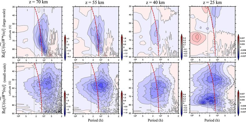
4.2.2 The meridional structure of the momentum flux
spectra
Next, the frequency spectra of vertical fluxes of the
zonal and meridional momentum (Re[U (ω)W ∗ (ω)],
Re[V (ω)W ∗ (ω)]) were obtained via the Blackman–
Tukey (1958) method. In Fig. 11, zonally averaged
Re[U (ω)W ∗ (ω)] and Re[V (ω)W ∗ (ω)] without diurnal and
semidiurnal migrating tides and semidiurnal non-migrating
tides with s = 1 are shown at heights of 70, 55, 40, and
25 km in JJA. Hereafter, these components are denoted as
^∗ (ω)] and Re[V (ω)W
Re[U (ω)W ^ ∗ (ω)], respectively. Note
Figure 8. Frequency power spectra of (a) zonal, (b) meridional, that the contributions of the tides to Re[U (ω)W ∗ (ω)] and
and (c) vertical wind and (d) temperature fluctuations averaged for Re[V (ω)W ∗ (ω)] are not large in the mesosphere during the
the height region of 70–75 km for JJA in NICAM at a grid point time period of JJA 2016 (not shown).
near Syowa Station. Vertical black dotted lines indicate frequencies
For Re[U (ω)W^∗ (ω)], an isolated peak is observed near
corresponding to 1 day and half a day. Red dotted lines indicate the
inertia frequency at Syowa Station (∼ 2π/12.7 h at 69◦ S). Error the inertial frequency from 55 to 75◦ S at a height of 70 km.
bars show intervals of the 90 % statistical significance. Another spectral peak at frequencies from 2π/10 to 2π/8 h
from 77 to 90◦ S appears to be similar to that of P fv (ω)
(Fig. 9). In addition, large spectral values are distributed
planetary waves, is found from the midlatitudes to the south near 55◦ S at frequencies from 2π/12 to 2π/6 h. The signs
pole. ^∗ (ω)] are mostly negative over the entire fre-
of Re[U (ω)W
The spectral peaks near the inertia frequency are also quency range. At heights of 55 and 40 km, there are large
found in the high-latitude region at a height of 55 km spectral values of Re[U (ω)W^∗ (ω)] from 65 to 75◦ S be-
(Fig. 9b). In addition, large spectral values are distributed in cause the isolated peaks are distributed around the inertial
the frequency range from the inertial frequencies to 2π/24 h frequency from 55 to 60◦ S but not from 65 to 75◦ S. At a
from 50 to 60◦ S but not from 30 to 40◦ S. The spectral height of 25 km, two separated spectral peaks are found at
peaks near the inertia frequency in the high-latitude region frequencies from 2π/24 to 2π/12 h. One is centered from 45
are barely seen at heights of 40 and 25 km, suggesting that to 55◦ S, while the other is centered from 65 to 80◦ S.
such spectral peaks in the high-latitude region are only found Conversely, the sign of Re[V (ω)W^ ∗ (ω)] at a height of
in the mesosphere. At a height of 25 km, the spectral values 25 km is negative from 45 to 55◦ S but positive from
are greatest in the inertial frequencies at midlatitudes from 65 to 80◦ S. Under the assumption of upward propa-
30 to 40◦ S, which is consistent with the result shown by Sato gation, it is likely that gravity waves with large nega-
et al. (1999) using a high-resolution GCM. Note that energy ^∗ (ω)] at a height of 25 km from 45 to
peaks at frequencies from 2π/10 to 2π/8 h in regions from tive Re[U (ω)W
77 to 90◦ S are seen at all heights. 55 S propagate poleward, while those from 65 to 80◦ S
◦
Here, we focus on the spectral peaks found in Fig. 9a near propagate equatorward. At heights of 40 and 55 km,
however, Re[V (ω)W ^ ∗ (ω)] around the spectral peak of
the inertial frequency from 65 to 75◦ S and at frequencies
from 2π/10 to 2π/8 h from 77 to 90◦ S. The horizontal map ∗
^(ω)] at slightly lower frequencies than the in-
Re[U (ω)W
of the integration of Pfv (ω) (i.e., the variance) for frequen- ertial frequency is mostly negative. These features suggest
cies from 2π/30 to 2π/12 h at a height of 70 km is shown that the two spectral peaks at a height of 25 km propagate
www.atmos-chem-phys.net/19/3395/2019/ Atmos. Chem. Phys., 19, 3395–3415, 20193406 R. Shibuya and K. Sato: A study of the dynamical characteristics of inertia–gravity waves Figure 9. Zonal mean ground-based frequency power spectra of meridional wind fluctuations without diurnal and semidiurnal migrating tides and semidiurnal non-migrating tides with s = 1 (P fv (ω)) averaged in JJA as a function of latitude at heights of (a) 25 km, (b) 40 km, (c) 55 km, and (d) 70 km. (e) Frequency spectra of temperature fluctuations averaged in June and July with horizontal wavelengths longer than 1000 km without the migrating tides at 70 km. Vertical black dotted lines indicate frequencies corresponding to the 1-day period and half day. A red thick dashed curve indicates the inertial frequencies at each latitude. Figure 10. The horizontal map of Pfv (ω) contributed by disturbances (a) at the frequencies from (2π/30 h) to (2π/12 h) and (b) at the frequencies from (2π/12 h) to (2π/6 h) at a height of 70 km. A red star denotes the location of Syowa Station. Atmos. Chem. Phys., 19, 3395–3415, 2019 www.atmos-chem-phys.net/19/3395/2019/
R. Shibuya and K. Sato: A study of the dynamical characteristics of inertia–gravity waves                                                 3407

Figure 11. Zonal mean ground-based frequency power spectra of vertical fluxes of zonal and meridional momentum (Re[U (ω)W ∗ (ω)],
Re[V (ω)W ∗ (ω)]) without diurnal and semidiurnal migrating tides, and semidiurnal non-migrating tides with s = 1 averaged in JJA as a
function of latitude at heights of 25, 40, 55, and 70 km. Vertical black dotted lines indicate frequencies corresponding to the 1-day period and
half day. A red thick dashed curve indicates the inertial frequencies at each latitude.

toward 60◦ S and then merge into an isolated spectral peak                tion of gravity waves discussed by Sato et al. (2009) and
at a height of 40 km. At heights from 40 to 70 km, gravity                Kalisch et al. (2014). However, gravity waves at frequencies
waves at frequencies lower than the inertial frequencies from             from 2π/30 to 2π/12 h propagate poleward above a height
60 to 90◦ S have negative Re[V (ω)W  ^    ∗ (ω)], while those at          of 40 km, not into the jet axis. This contrast is inherently re-
frequencies higher than the inertial frequencies have positive            lated to the existence of the isolated peaks around the inertial
       ^
Re[V (ω)W    ∗ (ω)]. From 30 to 60◦ S, gravity waves at fre-              frequency at heights of 55–70 km in Fig. 11, which is dis-
                                                                          cussed in detail in Sect. 5. Note that Re[ρ0 V (ω)W^   ∗ (ω)] at
quencies higher than the inertial frequencies have negative
       ^
Re[V (ω)W    ∗ (ω)].                                                      frequencies from 2π/12 to 2π/6 h has large negative values
   To examine these features, the latitude–height sections                near a latitude of 30◦ S at heights above 35 km. This may be
               ^∗ (ω)] and Re[ρ0 V (ω)W  ^    ∗ (ω)] for gravity
                                                                          related to the meridional propagation of convective gravity
of Re[ρ0 U (ω)W                                                           waves from the equatorial region, as suggested by an obser-
waves at frequencies from 2π/30 to 2π/12 h are shown in                   vational study using MF radar (Yasui et al., 2016).
Fig. 12a, while those from 2π/12 to 2π/6 h are shown in                                                    ^∗ (ω)] at frequencies from
                                   ^∗ (ω)] from both 2π/30                   A horizontal map of Re[U (ω)W
Fig. 12b. It is seen that Re[ρ0 U (ω)W                                    2π/30 to 2π/12 h at a height of 25 km is shown in Fig. 13a,
to 2π/12 h and 2π/12 to 2π/6 h has two branches in the                    while that at frequencies from 2π/12 to 2π/6 h is shown in
lower stratosphere, which merge southward of the polar night
jet axis at a height of approximately 40 km. The signs of                 Fig. 13b. At latitudes from 65 to 80◦ S, Re[U (ω)W
                                                                                                                           ^∗ (ω)] has
          ^     ∗ (ω)] at frequencies from 2π/30 to 2π/12 h
                                                                          very large negative values above the Antarctic Peninsula in
Re[ρ0 V (ω)W                                                                                                                ^∗ (ω)] are
are positive (negative) at heights below 40 km along the low-             both Fig. 13a and b. Negative values of Re[U (ω)W
                                               ^∗ (ω)], while             also found along the coast of Antarctica, in particular, above
latitude (high-latitude) branch of Re[ρ0 U (ω)W                           the western side of the Ross Sea. Therefore, it is thought that
they are primarily negative at heights above 40 km. Con-                                                      ^∗ (ω)] shown in Fig. 12
                                ^    ∗ (ω)] at frequencies from
                                                                          the poleward branches of Re[U (ω)W
versely, the signs of Re[ρ0 V (ω)W                                        are primarily due to orographic gravity waves. However, note
2π/12 to 2π/6 h are positive (negative) poleward (equator-                that the gravity waves observed over the coast of Antarctica
ward) of 60◦ S from the lower stratosphere to the meso-                   may be partly due to non-orographic gravity waves caused by
sphere. These results indicate that gravity waves at frequen-             spontaneous radiation from the upper tropospheric jet stream
cies from 2π/12 to 2π/6 h propagate into 60◦ S, which is                  (Shibuya et al., 2016).
similar to the previous picture of the meridional propaga-

www.atmos-chem-phys.net/19/3395/2019/                                                        Atmos. Chem. Phys., 19, 3395–3415, 2019
3408 R. Shibuya and K. Sato: A study of the dynamical characteristics of inertia–gravity waves
^
Figure 12. Latitudinal structures of an integration of Re[ρ0 U (ω)W ∗ (ω)] and Re[ρ V (ω)W
^ ∗ (ω)] contributed by wave disturbances (a) for
0
the frequencies from (2π/30 h) to (2π/12 h) and (b) for the frequencies from (2π/12 h) to (2π/6 h) averaged in JJA. The contour values
indicate zonal mean zonal wind with a contour interval of 30 m s−1 .
Figure 13. The horizontal map of Re[ρ0 U (ω)W^ ∗ (ω)] contributed by disturbances (a) at the frequencies from (2π/30 h) to (2π/12 h) and
(b) at the frequencies from (2π/12 h) to (2π/6 h). Regions surrounded by red rectangles and green rectangles denote the domain dominated
by the topography and the island, respectively.
To examine the contribution of orographic and non- of Re[U (ω)W^∗ (ω)] is likely primarily composed of non-
orographic gravity waves to the equatorward branches in orographic gravity waves.
Fig. 12, the magnitudes of Re[U (ω)W ^∗ (ω)] from 42 to Finally, the horizontal scales of the wave disturbances con-
57◦ S (the thick black circles in Fig. 13) were estimated ^∗ (ω)] were examined at each height.
tributing to Re[U (ω)W
over various topographies (the red rectangles), islands (the Hereafter, small- to medium-scale (large-scale) wave dis-
green rectangles), and the Southern Ocean. The decompo- turbances are defined as components with horizontal wave-
sition of these domains is also described in Fig. 13. Over lengths smaller than (larger than) 1000 km, as occasionally
the latitudinal band from 42 to 57◦ S, the contributions of defined in previous studies (e.g., Geller et al., 2013). To ex-
^∗ (ω)] due to gravity waves at frequencies from
Re[U (ω)W tract the small- to medium-scale and large-scale components,
2π/30 to 2π/12 h over the topographies, islands, and South- a spatial filter was applied to the wind data gridded in an x–
ern Ocean are 12.3 %, 6.6 %, and 81.1 %, respectively, while y coordinate system centered at the South Pole as projected
those at frequencies from 2π/12 to 2π/6 h are 7.1 %, 6.0 %, by the Lambert azimuthal equal-area projection. Figure 14
and 86.9 %, respectively. Therefore, the equatorward branch shows the zonally averaged Re[U (ω)W ^∗ (ω)] resulting from
Atmos. Chem. Phys., 19, 3395–3415, 2019 www.atmos-chem-phys.net/19/3395/2019/R. Shibuya and K. Sato: A study of the dynamical characteristics of inertia–gravity waves 3409
Figure 14. Zonal mean ground-based frequency power spectra of vertical fluxes of zonal momentum (Re[U (ω)W ∗ (ω)]) without diurnal and
semidiurnal migrating tides and semidiurnal non-migrating tides with s = 1 averaged in JJA as a function of latitude at heights of 25, 40, 55,
and 70 km. The upper (lower) line shows Re[U (ω)W ∗ (ω)] contributed by disturbances with horizontal scales larger (smaller) than 1000 km.
A red thick dashed curve indicates the inertial frequencies at each latitude.
large-scale and small- to medium-scale components during this study, Pw (ω) simulated by NICAM, as shown in Fig. 8c,
JJA at heights of 70, 55, 40, and 25 km. At heights of 25 is consistent with the PANSY radar observations. Moreover,
and 40 km, it appears that the majority of Re[U (ω)W ^∗ (ω)] Sato et al. (2017) demonstrated that the power spectrum of
is composed of small- to medium-scale components, while the vertical flux of the zonal momentum (Re[U (ω)W ∗ (ω)])
at heights of 55 and 70 km, the large-scale components have has a positive isolated peak near the inertial frequency in the
large negative values near the inertial frequencies. This fea- eastward background zonal wind in the summer season. The
ture is consistent with Shibuya et al. (2017), who showed that shape of Re[U (ω)W ∗ (ω)] shown in NICAM is consistent
mesospheric disturbances with a large amplitude observed with the results of Sato et al. (2017), even though the sign
at Syowa Station are due to quasi-12 h gravity waves with shown in this study is negative under the westward back-
horizontal wavelengths larger than 1500 km. In addition, it ground zonal wind in winter. Conversely, using the Fe Boltz-
appears that the spectral peak at frequencies from 2π/8 to mann lidar at McMurdo Station (166.7◦ E, 77.8◦ S), Chen
2π/10 h for the latitude range from 77 to 90◦ S is also due to et al. (2016) showed that Pt (ω) has a broad spectrum peak
large-scale wave disturbances. at frequencies from 2π/3 to 2π/10 h centered at approxi-
mately 2π/8 h at a height of 85 km in June for the 5 years
of 2011–2015, which is also consistent with the Pt (ω) result
5 Discussion ^
in Fig. 8d. The latitude–height section of Re[ρ0 V (ω)W ∗ (ω)]
in Fig. 12b indicates that the spectral peak from 2π/3 to
Recently, Sato et al. (2017) estimated the power spectra 2π/10 h is composed of gravity waves originating over the
of horizontal and vertical wind fluctuations and momentum Antarctic continent. These results indicate that the spectra of
flux spectra over a wide frequency range from 2π/8 min to the mesospheric disturbances simulated in NICAM are very
2π/20 days using continuous PMSE observation data from realistic at high latitudes in the Southern Hemisphere.
the PANSY radar over three summer seasons. It was shown The spectral peaks of Pv (ω) without the migrating tides
that the spectral slope of Pw (ω) at frequencies from 2π/2 h in the mesosphere are simulated near the inertial frequen-
to 2π/5 days is nearly flat in the height range of 84–88 km, cies at latitudes from 30 to 75◦ S. Therefore, the quasi-12 h
which is particularly clear in the spectra of observations by inertia–gravity waves at Syowa Station examined by Shibuya
the full PANSY system in the 2015–2016 austral summer et al. (2017) can be interpreted as quasi-inertial period grav-
season. Even though the altitude range and season exam- ity waves. Moreover, it is shown that Re[U (ω)W ∗ (ω)] also
ined by Sato et al. (2017) are different from those studied in
www.atmos-chem-phys.net/19/3395/2019/ Atmos. Chem. Phys., 19, 3395–3415, 2019You can also read