SAFIRE ATR 42 aircraft - The EUREC4A turbulence dataset derived from the - ESSD
←
→
Page content transcription
If your browser does not render page correctly, please read the page content below
Earth Syst. Sci. Data, 13, 3379–3398, 2021
https://doi.org/10.5194/essd-13-3379-2021
© Author(s) 2021. This work is distributed under
the Creative Commons Attribution 4.0 License.

             The EUREC4 A turbulence dataset derived from the
                         SAFIRE ATR 42 aircraft
          Pierre-Etienne Brilouet1 , Marie Lothon1 , Jean-Claude Etienne2 , Pascal Richard2 , Sandrine Bony4 ,
          Julien Lernoult3 , Hubert Bellec3 , Gilles Vergez3 , Thierry Perrin3 , Julien Delanoë5 , Tetyana Jiang3 ,
           Frédéric Pouvesle3 , Claude Lainard3 , Michel Cluzeau3 , Laurent Guiraud3 , Patrice Medina1 , and
                                                     Theotime Charoy3
                          1 Laboratoired’Aérologie, University of Toulouse, CNRS, UPS, Toulouse
                                         2 CNRM, Météo-France, CNRS, Toulouse
                                    3 SAFIRE, CNRS, Météo-France, CNES, Toulouse
                                 4 LMD/IPSL, CNRS, Sorbonne University, Paris, France
           5 Laboratoire Atmosphères, Milieux, Observations Spatiales/UVSQ/CNRS/UPMC, Guyancourt, France

                              Correspondence: Marie Lothon (marie.lothon@aero.obs-mip.fr)

                                  Received: 17 February 2021 – Discussion started: 1 March 2021
                              Revised: 1 June 2021 – Accepted: 3 June 2021 – Published: 14 July 2021

       Abstract. During the EUREC4 A field experiment that took place over the tropical Atlantic Ocean east of Bar-
       bados, the French ATR 42 environment research aircraft of SAFIRE aimed to characterize the shallow cloud
       properties near cloud base and the turbulent structure of the subcloud layer. For this purpose, the aircraft payload
       included radar and lidar remote sensing, microphysical probes, a laser spectrometer, and meteorological sensors.
       In particular, the aircraft was equipped with a five-hole radome nose as well as several temperature and moisture
       sensors allowing for measurements of wind, temperature and humidity at 25 Hz. This paper presents the high-
       frequency measurements made with these sensors and their translation in terms of turbulent fluctuations, turbu-
       lent moments and characteristic length scales of turbulence. A particular focus is on the calibration and the qual-
       ity control of the air moisture measurements, which remain a challenge at fine scales. Level-2 and Level-3 data
       are distributed as an ensemble of NetCDF files available to the public at AERIS (https://doi.org/10.25326/128,
       Lothon and Brilouet, 2020).

1   Introduction                                                   wind clouds are known to organize in various mesoscale pat-
                                                                   terns (referred to as “Sugar”, “Gravel”, “Fish” or “Flow-
                                                                   ers”) that embed different cloud types and depend on en-
For many decades, difficulties in quantifying the strength of      vironmental conditions (Stevens et al., 2020; Bony et al.,
the low-level cloud feedback, especially in the trade-wind         2020). LeMone and Pennell (1976) and LeMone and Meitin
regions, have hindered precise estimates of the climate sen-       (1984) suggested that shallow cloud organization could also
sitivity. Improving our estimate of the feedback requires a        be rooted in the structure of the subcloud layer. For in-
better understanding of the physical processes that control        stance, LeMone and Pennell (1976) showed that in highly
cloudiness in the trades and their dependence on environ-          suppressed conditions, the cloud distribution was related to
mental conditions. The low-level clouds that form in the           the organization of the subcloud layer in structures such as
trade-wind regimes are closely associated with shallow cu-         roll vortices. In contrast, in situations of enhanced convection
mulus convection, and early studies by Malkus (1958) and           the turbulence seemed to be more directly and locally linked
LeMone and Pennell (1976) showed that the properties of            to individual clouds. The state of the subcloud layer thus
trade cumuli could be understood to a large extent by exam-        seems to influence the degree of coupling (or decoupling) be-
ining the properties of the subcloud layer. Moreover, trade-

Published by Copernicus Publications.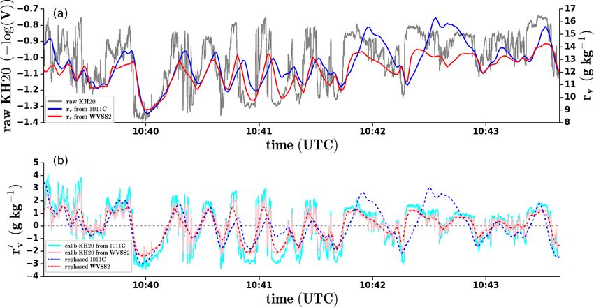
3380                                                                P.-E. Brilouet et al.: The EUREC4 A ATR 42 turbulence dataset

tween the surface and clouds and thus the cloud distribution.
However, accurate and intensive observations are needed to
further elucidate the connection between the mesoscale cloud
patterns, the subcloud layer and the surface.
   The EUREC4 A field campaign was designed to bet-
ter understand what controls the trade-wind cloudiness, its
mesoscale organization, and its interplay with convection
and circulations over a wide range of scales (Bony et al.,
2017). The experiment took place in January–February 2020
over the tropical western Atlantic east of Barbados. Many
observing systems were deployed during the campaign, in-
cluding four research aircraft, four research vessels, and a
large number of autonomous observing systems in the ocean
and in the atmosphere (Stevens et al., 2021). One of the
aircraft was the ATR 42 operated by the French Research
Aircraft Infrastructure for Environmental Studies (SAFIRE).
During the campaign, its mission was primarily devoted to
the characterization of the shallow cloudiness near cloud
base (Chazette et al., 2020; Bony et al., 2017; Stevens et
                                                                        Figure 1. Schematic horizontal trajectory of the SAFIRE ATR 42
al., 2021) and the turbulent properties of the subcloud layer.
                                                                        within the HALO circle (gray dashed lines) during EUREC4 A. Ma-
Its flights were closely coordinated with those from HALO,              neuvers for alignment, ferry legs and other parts of the trajectory
the German research aircraft, which was flying large cir-               projection are not shown here. The R pattern is shown in red, and
cles at a higher altitude to observe clouds from above and              the L pattern is shown in blue.
to characterize the dynamical and thermodynamical environ-
ment through intensive dropsonde measurements (Konow et
al., 2021). The characterization of the turbulence within the           2    Flight strategy and conditions
marine atmospheric boundary layer (MABL) plays a major
role in EUREC4 A, as it will help decipher the interactions             The core experimental strategy of the EUREC4 A field cam-
between turbulence, convection and clouds, as well as the               paign was based on the coordination of the SAFIRE ATR
dependence of clouds on surface and large-scale conditions.             42 and HALO aircraft: while HALO was flying large circles
Moreover, the MABL being the interface between the ocean                (200 km diameter, referred to as EUREC4 A circles) at an al-
surface and the cloud layer, the characterization of its turbu-         titude of about 9 km (Konow et al., 2021), the SAFIRE ATR
lent structures should also help understand how mesoscale               42 was flying in the lower troposphere of the western half of
and sub-mesoscale heterogeneities at the ocean surface, as-             the circle, describing two types of pattern (Fig. 1):
sociated with the presence of ocean eddies or sea surface
temperature fronts, could imprint themselves in the cloud or-               – an “R pattern” composed of at least two rectangles (of
ganization aloft.                                                             about 120 km by 15 km) flown at cloud base to char-
   This paper describes the EUREC4 A dataset containing the                   acterize the cloud-base cloud fraction through horizon-
turbulent fluctuations and turbulent moments associated with                  tally staring lidar and radar measurements and
the high-frequency measurements of temperature, moisture
and wind from the SAFIRE ATR 42 aircraft computed over                      – an “L pattern” flown within the subcloud layer at two
horizontal stabilized legs. Section 2 describes the flight strat-             different heights to characterize the turbulence and the
egy and the type of meteorological and cloud conditions                       coherent structures of the boundary layer.
encountered during the flights. Section 3 presents the in situ
instrumentation. Sections 4 and 5 explain the quality control           At the end of most flights, these two patterns were completed
procedure and the calibration methodology used to process               by a short surface leg (“S leg”) flown at 60 m above sea level
the moisture and temperature fluctuations. Section 6 explains           before returning to the airport.
how the turbulent moments are computed and how their sys-                  During each SAFIRE ATR 42 flight, two to four rectan-
tematic and random errors are quantified. Length scales char-           gles were flown, generally around the cloud-base level, ex-
acteristic of the turbulent field are also estimated. Section 7         cept when stratiform clouds were occurring higher up and a
describes the turbulence dataset in more detail and shows               rectangle was also flown around the trade inversion level. In
a few illustrations of its content. A conclusion is given in            addition, two to four L patterns were flown, each pattern be-
Sect. 8.                                                                ing composed of two straight legs of about 60 km (one along-
                                                                        wind and one across-wind) flown either near the top or the
                                                                        middle of the subcloud layer. These patterns aimed to ex-

Earth Syst. Sci. Data, 13, 3379–3398, 2021                                               https://doi.org/10.5194/essd-13-3379-2021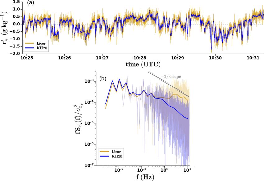
P.-E. Brilouet et al.: The EUREC4 A ATR 42 turbulence dataset                                                               3381

plore the anisotropy of the turbulence and the organization,       scribed by Brown et al. (1983). The true air speed (TAS)
as well as the vertical structure of the boundary layer.           is calculated from the measurement of the dynamical pres-
   During a single HALO flight of about 9 h, the ATR 42 flew       sure and the static pressure. The static pressure is measured
two flights (using a similar flight plan) with a short refueling   on the fuselage side with a Pitot tube and a pressure trans-
in between. The repetitiveness of the flight plans makes it        ducer. The dynamical pressure is obtained by subtracting the
possible to consider all the flights to be members of the same     static pressure from the total pressure measured at the cen-
statistical ensemble.                                              tral radome hole. The velocity measurement and computa-
   Table 1 describes each flight plan, together with some in-      tion have proven to be reliable in numerous field campaigns
formation about the mean wind within the subcloud layer            (Lambert and Durand, 1998; Saïd et al., 2005, 2010).
and the types of clouds observed. It shows how, during the             Air temperature is retrieved from a platinum wire ther-
campaign, the conditions evolved from suppressed condi-            mometer placed in a Rosemount housing (E102AL Rose-
tions, with only rare and thin cumulus clouds, toward more         mount), after correction for the adiabatic heating due to the
cloudiness and more vertical development. This was associ-         air speed of the plane. During EUREC4 A, temperature was
ated with a gradual strengthening of the mean wind in the          also measured using two fine wires (Baehr et al., 2002) that
subcloud layer. Note that flights RF01 and RF02 are not in-        were housed in a tubular antenna. The two platinum fine
cluded in the table because they were electromagnetic inter-       wires are housed in a tubular antenna from SFIM company
ference (EMI) and test flights, and RF20 had no rapid mea-         (model T4113). They are more directly exposed to the stream
surements because of an inertial navigation system failure.        but protected from radiation, which consequently should not
                                                                   have a significant impact.
                                                                       Moisture fluctuations were measured with a krypton hy-
3   Aircraft in situ instrumentation for high-rate                 grometer Campbell KH20, which has been adapted for air-
    thermodynamical measurements                                   planes. Initially used for measurements on ground towers,
                                                                   this sensor was profoundly modified to be inserted into the
The SAFIRE ATR 42 is a turboprop airplane initially used for       housing of a former moisture sensor (Lyman-alpha hygrom-
commercial aviation, which has been profoundly modified            eter). The signal is calibrated based on reference slow (1 Hz)
for the purpose of atmospheric and environmental research.         measurements of humidity. Here we use the Water Vapor
It is permanently instrumented with in situ basic measure-         Sensing System (WVSS2) for reference instead of the typi-
ments (thermodynamics, radiation, microphysics) and also           cal chilled-mirror sensor reference (General Eastern 1011). A
has a large flexible payload capacity, which enables the use       Li7500 LI-COR sensor was used as a spare for fast humidity
of a large number of in situ and remote sensing observations.      measurements. It was also adapted for aircraft measurements
   The core in situ instrumentation used during EUREC4 A           and previously used in the HyMeX (Estournel et al., 2016)
and the low-rate measurements (1 Hz) associated with it are        and DACCIWA (Knippertz et al., 2015) field campaigns.
described in Bony et al. (2017) and Stevens et al. (2021).             Due to several circumstances, some technical difficulties
The higher-rate measurements (25 Hz) are, to a large extent,       were encountered during the field campaign, especially dur-
based on the same instrumentation.                                 ing its first phase. In particular, a major issue concerned one
   The SAFIRE ATR 42 is equipped for high-rate measure-            of the radome pressure transducers, making it impossible to
ments of the three wind components of air motion, air tem-         calculate the attack angle with the usual methodology. This
perature and air moisture. Initially acquired at various higher    strongly impacts the air vertical velocity estimates. As a con-
sampling rates consistent with the time response of the sen-       sequence and due to the sensitivity of air motion measure-
sors, the final high-rate measurements of the meteorologi-         ments, the dataset discussed here does not include the vertical
cal variables were sampled at a common frequency of 25 Hz.         velocity for flights RF02 to RF08, nor any estimate related to
For a true air speed of about 100 m s−1 , this corresponds to a    it.
sample spacing of approximately 4 m.                                   The KH20 also showed issues during this first phase,
   The three components of the wind are obtained by adding         partly due to the particular conditions of the marine en-
the velocity vector of the aircraft with respect to the Earth      vironment encountered during EUREC4 A, which make it
and the velocity vector of the air with respect to the aircraft.   challenging to measure air moisture at fine scale. The dras-
The ground velocity is measured with an inertial navigation        tic change in water vapor content from above the inversion
unit (AIRINS, model 6005214 from iXblue company). The              (where relative humidity can be as dry as a few percent)
velocity of the air relative to the aircraft is computed from      to below cloud base (where relative humidity is generally
the measurement of the true air speed magnitude as well            higher than 80 %) was a challenge, and the spacing between
as the attack and side-slip angles, according to Lenschow          the emitter and the receiver of the KH20 sensor has been ad-
(1986). The attack and side-slip angles are respectively de-       justed. In the subcloud layer patterns, the sea salt loading of
duced from the vertically aligned and horizontally aligned         the KH20 sensor generated a significant loss of signal dy-
differential pressure measured on the five-hole nose radome        namics. An assiduous cleaning of the optics at the beginning
with pressure transducers, according to the technique first de-    of each flight allowed us to limit this loss of signal. Regard-

https://doi.org/10.5194/essd-13-3379-2021                                         Earth Syst. Sci. Data, 13, 3379–3398, 2021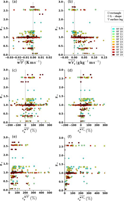
3382 P.-E. Brilouet et al.: The EUREC4 A ATR 42 turbulence dataset
Table 1. Flight plan and wind conditions associated with each flight during the EUREC4 A field campaign. The flight altitude is indicated be-
tween brackets, and the notations “cb”, “strati” and “surf” refer to cloud base, stratiform layer and surface, respectively. The wind conditions
within the subcloud layer are inferred from the averaged airborne measurements over the L legs, including both the top and mid-subcloud
layer (except for RF16, during which there was no L pattern). ti and tf are UTC times for the start and end of the flights, respectively.
RF Date ti tf Flight strategy Wind conditions Cloud cover
2Rcb (800 m) Small cloudiness
03 26 January 11:59 16:04 7.2 ± 0.8 m s−1
3L (580, 400, 60 m) Scarce and very thin Cu
3Rcb (800 m) Small cloudiness
04 26 January 16:57 21:26 3.5 ± 0.7 m s−1
2L (600, 400 m) + Lsurf (60 m) Scarce and very thin Cu
2Rcb (670 m) Small cloudiness
05 28 January 20:36 24:50 7.8 ± 0.6 m s−1
2L (450, 300 m) + Lstrati (1800 m) Getting smaller with time
3Rcb (650–750 m) Scattered ShCu
06 30 January 11:11 15:31 8.9 ± 0.5 m s−1
2L (550, 300 m) + Lsurf (60 m) Less cloudy with time
2Rcb (600 m) + 1/2Rcb (700 m) Sparse Cu at the
07 31 January 14:59 18:48 7.9 ± 0.7 m s−1
2L (400, 200 m) edge of cold pools
3Rcb (550–610 m) Mostly ShCu
08 31 January 19:49 24:01 6.6 ± 0.6 m s−1
2L (450, 300 m) Few towering clouds
2Rcb (600 m)
09 2 February 11:34 15:37 7.4 ± 1.4 m s−1 Heterogeneous
2L (300, 600 m) + 1/2L (600 m) + Lstrati (1100 m)
3Rcb (710–770 m)
10 2 February 16:44 21:03 5.4 ± 0.8 m s−1 Heterogeneous
2L (580, 300 m) + Lsurf (60 m)
Rstrati (1830 m) + 2Rcb (680–740 m) Succession of
11 5 February 08:45 12:59 10.8 ± 1.0 m s−1
2L (530, 250 m) + Lsurf (60 m) Flower clouds
3Rcb (790 m) Increase in the
12 5 February 13:48 18:04 9.4 ± 0.4 m s−1
2L (550, 250 m) + Lsurf (60 m) cloud fraction
Rstrati (2100 m) + 2Rcb (750 m)
13 7 February 11:30 15:51 12.3 ± 1.0 m s−1 Heterogeneous
2L (540, 60 m) + 2L1/2 (280 m, 575 m)
3Rcb (980–775 m)
14 7 February 17:20 21:42 11.0 ± 0.4 m s−1 Heterogeneous
2L (640, 330 m) + Lsurf (60 m)
3Rcb (820 m) Patchy clouds
15 9 February 08:37 13:08 10.9 ± 0.4 m s−1
2L (620, 300 m) + Lsurf (60 m) Few cold pools and strati layers
4Rcb (800 m) Patchy clouds
16 9 February 14:03 18:23 11.8 ± 0.7 m s−1
Lsurf (60 m) Few cold pools and strati layers
Rstrati (1800 m) + 2Rcb (700 m)
17 11 February 05:55 10:21 12.5 ± 0.7 m s−1 Active convective cells
2L (570, 285 m)
3Rcb (775 m) Multi-layer ShCu,
18 11 February 11:30 15:50 10.9 ± 0.4 m s−1
2L (560, 265 m) + Lsurf (60 m) tower Cu and strati layers
Rstrati (1850 m) + 2Rcb (790–855 m) Cloud conditions with
19 13 February 07:35 11:51 12.8 ± 0.7 m s−1
2L (600, 300 m) StCu and towering Cu
For the description of the cloud cover, the abbreviations are defined as follows. Cu: cumulus, ShCu: shallow cumulus, StCu: stratocumulus, Flower clouds: circular clumped patterns as
introduced by Stevens et al. (2020).
ing the KH20 behavior, many technical issues were gradu- As a consequence of those difficulties and after quality
ally solved and several improvements were made following control, there are flagged or rejected data within the dataset.
the feedbacks at the end of each flight. Thus, the KH20 per- The second phase of the field, corresponding to flights RF09
formances were significantly improved by the second phase to RF19, had much better-quality data.
of the campaign (flights RF09 to RF19). The calibration of
moisture fluctuations, choice of reference slow measurement,
and the relative performances of the KH20 and LI-COR are
discussed further in Sect. 4.
Earth Syst. Sci. Data, 13, 3379–3398, 2021 https://doi.org/10.5194/essd-13-3379-2021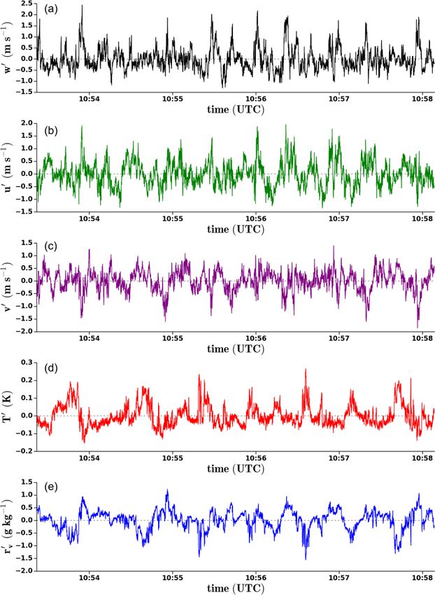
P.-E. Brilouet et al.: The EUREC4 A ATR 42 turbulence dataset 3383
4 Calibration and qualification of the fast humidity The latter, despite its shorter response time, showed more
sensors difficulties in following the large variability of air moisture
encountered during EUREC4 A, which added to the chal-
One of the current challenges of atmospheric turbulence lenges of measuring air moisture in an environment with sea
measurements is the fast measurement of humidity, which salt, clouds or even rain. This phenomenon can be noticed
remains difficult at frequencies higher than 1 Hz. For many around 10:29:20 UTC in Fig. 2b and more clearly in Fig. 3,
years in the past, a robust and high-performance krypton where the 1011C signal (dashed blue) shows several exagger-
hygrometer called Lyman-alpha was commonly used for ated peaks because it responded too slowly to the increasing
the measurement of (uncalibrated) air moisture fluctuations and following fast leveling of moisture. This behavior is ex-
(Buck, 1976; Saïd et al., 2010; Canut et al., 2010). Since the plained by its measurement principle, with condensation at
UV source of this sensor is not available anymore, one had the mirror surface, which requires time to recover by drying.
to use another sensor. However, achieving a similar perfor- This issue resulted in a positive bias of about 27 % in the
mance remains a challenge. Here, we use a KH20 krypton estimated moisture variance when the KH20 was calibrated
hygrometer, which has been recently adapted and installed with the 1011C hygrometer. This bias is visible in Fig. 2b
on board the SAFIRE ATR 42. and even more clearly in Fig. 3b from the difference in fluc-
In this section, we discuss the data calibration and control tuation energy between the two signals.
over stabilized legs of 5 min. This segmentation is a compro- Figure 4 makes the distinction between legs flown within
mise to ensure the best sampling representativity and homo- the subcloud layer (or MABL legs, associated with more ho-
geneity (see Sect. 6 for more details). mogeneous turbulence) and the rest of the legs. At cloud
The time series shown in Fig. 2a illustrates a compari- base, the turbulence is highly heterogeneous, with a mix of
son of uncalibrated fast measurements from the KH20 sen- cloudy air, subcloud layer air and free tropospheric air. On
sor with two slow sensors: the WVSS2 sensor and the 1011C the other hand, the legs flown higher up near the trade inver-
mirror hygrometer. The WVSS2 measures the relative hu- sion level exhibit a very weak turbulence or an intermittent
midity in percent by absorption spectroscopy with a tunable turbulence associated with individual clouds. The distribu-
diode. The 1011C hygrometer is a condensation hygrome- tions do not show strong differences between one set and the
ter, which measures the dew point temperature. Absolute, other. This indicates that the calibration against WVSS2 ac-
relative and specific humidity are then inferred from dew tually works both in the MABL and above the subcloud layer.
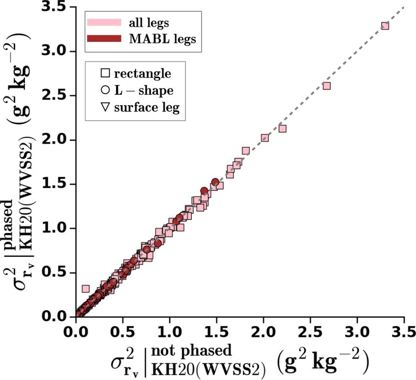
point, temperature and pressure. To calibrate the fast sensor The WVSS2 is a slower sensor than the 1011C hygrom-
with the reference slow measurement of absolute humidity, eter, with a time response of about 2.5 s against about 1 s.
both the slow and fast signals are initially low-pass-filtered Due to this significant delay (that can be seen in Fig. 2a), we
at 1/6 Hz, and then a linear regression is computed to ob- tested the impact of phasing the slow signal to the fast signal.
tain the calibration slope and the intercept to be applied to Figure 4c shows the significant improvement obtained with
the fast signal. The quality of the calibration is assessed by this phasing: for most of the legs, R 2 is now larger than 0.95.
the R-squared value (R 2 ) of the linear regression between the Figure 2b shows the calibrated signal of the KH20 converted
low-pass signals of the reference sensor and of the fast sen- to a water vapor mixing ratio, along with the phased slow
sor. One expects R 2 larger than 0.98 for high-quality signals signal used for optimum calibration. Figure 5 shows that the
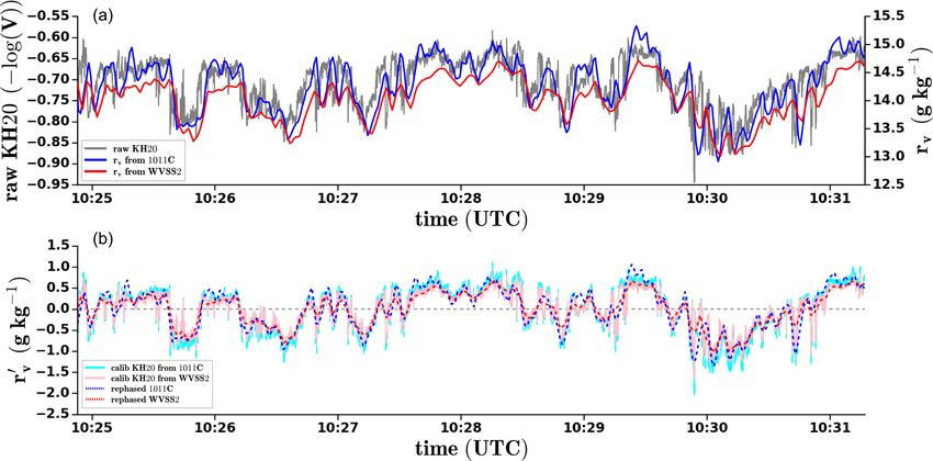
of slow and fast measurements. Figure 2b shows the result- phasing has only a small impact on the variance of moisture:
ing calibrated signal converted to a water vapor mixing ratio it is only 1.7 % larger in the case of the phased slow signal,
and compared to the slow series of the same variable. which is much smaller than the random error.
For a thorough qualification of the fast moisture measure-
4.1 Choice of slow sensor ments during EUREC4 A, considering R-squared values is
not sufficient. Indeed, even if the correlation with the slow
The measurements of the two slow sensors exhibit differ- signal is good, the sensor might not show the proper dynam-
ences which can impact the calibration. To optimize the ics of the amplitude of the fluctuations (e.g., due to sea salt
choice of the slow reference and the calibration process, we or to an inappropriate spacing between the emitter and the
considered the second phase of the campaign (flights RF09 receiver). For this reason, we used as an additional index,
to RF19), which had fewer technical issues and during which the root mean squared error (RMSE), calculated between the
the KH20 showed a very good behavior in terms of time low-pass-filtered calibrated signal (1/6 Hz) and the slow ref-
response and consistency with other moisture sensors. Fig- erence signal (also low-passed). The smaller this index, the
ure 4a and b show the distributions of R 2 on all segments of better the agreement between the fast and slow sensors at
flights RF09 to RF19 when using either the 1011C mirror hy- large scales.
grometer or the WVSS2 sensor as a reference, respectively. The quality of the fast humidity measurements is thus as-
The R 2 values are significantly higher when the WVSS2 sessed with respect to two metrics: R 2 and RMSE. For each
sensor is used as a reference. This reveals a better behav- sensor (KH20 or LI-COR), we define a green, yellow or red
ior of the WVSS2 sensor relative to the 1011C hygrometer. flag with respect to the combination of criteria for those two
https://doi.org/10.5194/essd-13-3379-2021 Earth Syst. Sci. Data, 13, 3379–3398, 2021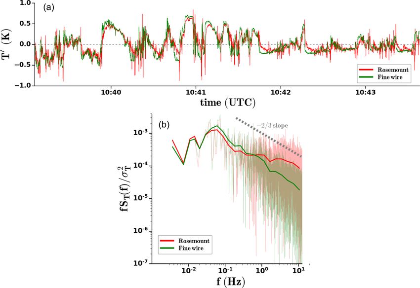
3384                                                                P.-E. Brilouet et al.: The EUREC4 A ATR 42 turbulence dataset

Figure 2. Example of humidity measurements and calibration during a leg (l1a) flown at z ∼ 600 m on 13 February 2020 (RF19): (a) time
series of (gray line) the raw uncalibrated signal of the fast KH20 sensor and the water vapor mixing ratio inferred from (blue line) the 1011C
mirror hygrometer or (red line) the WVSS2 sensor. (b) Corresponding time series of the water vapor mixing ratio fast fluctuations derived
from the KH20 calibrated signal and the reference slow measurements phased in time with the fast sensor from (cyan line) the 1011C mirror
hygrometer and (pink line) the WVSS2 sensor.

Figure 3. Same as Fig. 2 for a leg (l1c) flown at z ∼ 600 m on 13 February 2020 (RF19).

metrics (Fig. 6). The high-quality (green) flag is defined by            4.2    Comparison of the KH20 and LI-COR sensors
R 2 ≥ 0.9 and RMSE < 0.16. In contrast, the poor-quality
(red) flag is defined by R 2 < 0.6 or RMSE > 0.6. All other              During EUREC4 A, two fast sensors were mounted on the
combinations of those two metrics correspond to an interme-              SAFIRE ATR 42: the LI-COR sensor, which had been pre-
diate yellow flag. Note that the threshold values used to de-            viously adapted to the airplane, and the KH20 sensor, which
fine these criteria result from a sensitivity analysis that com-         was adapted to the airplane more recently in the hope of im-
pares the moisture flux and the variance obtained with the               proving the performance of the high-rate humidity measure-
KH20 or LI-COR sensors.                                                  ments.
                                                                            Figure 7a shows an example of time series from both sen-
                                                                         sors during a subcloud layer segment of flight RF19 after
                                                                         the calibration process discussed previously. First, it shows

Earth Syst. Sci. Data, 13, 3379–3398, 2021                                                 https://doi.org/10.5194/essd-13-3379-2021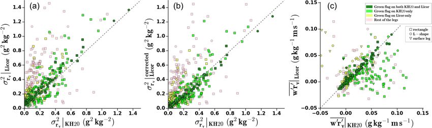
P.-E. Brilouet et al.: The EUREC4 A ATR 42 turbulence dataset                                                                            3385

Figure 4. Histograms of the linear regression R-squared value (R 2 ) associated with the calibration of the KH20 fast humidity measurement
with, as the reference slow measurement, (a) the 1011C mirror hygrometer, (b) the WVSS2 sensor and (c) the WVSS2 sensor phased in time
with the fast sensor. The comparison is done for all flights from RF11 to RF19, considering either the entire set of legs or just the legs flown
within the MABL. The vertical dashed line represents the R 2 = 0.9 threshold.

                                                                          Figure 6. For each sensor (KH20 or LI-COR), the quality of high-
                                                                          rate humidity measurements is assessed against two metrics: R 2 (on
                                                                          the horizontal axis) and RMSE (on the vertical axis). The quality
                                                                          decreases from green to red.
Figure 5. Variance of the water vapor mixing ratio computed with
the KH20 sensor, after calibration with the WVSS2 sensor phased
in time, versus the variance obtained when the WVSS2 sensor is
not phased. The comparison is done for all flights from RF11 to
                                                                             The determination of the thresholds of R 2 and RMSE for
RF19, considering either the entire set of legs or just the legs flown
within the MABL. The markers refer to the different types of leg,         the green flag introduced above was made such that the se-
as sketched in Fig. 1.                                                    lected green-flagged legs showed good consistency between
                                                                          the KH20 and the LI-COR for the estimates of moisture vari-
                                                                          ance and covariance. This is illustrated with Fig. 8. Con-
                                                                          sistently, when we consider only the legs with green flags
that the signal from the LI-COR sensor was associated with                for both sensors, the agreement on variance (Fig. 8a) and
significant noise. This feature was present during the en-                moisture flux (Fig. 8c) is very good, especially relative to
tire field campaign. In addition to this noise issue, the LI-             the small intensity of turbulence found in EUREC4 A and the
COR showed appropriate moisture measurements at lower                     large associated random errors.
frequencies, consistent with good R-squared coefficients of                  The noise of the LI-COR signal naturally impacts the
the calibration (R 2 = 0.99 for both KH20 and LI-COR in                   variance estimates, leading to an overestimation of about
Fig. 7). The corresponding spectra of those series shown in               0.05 g2 kg−2 (Fig. 8a). However, the LI-COR noise does not
Fig. 7b exhibit the noise issue of the LI-COR more clearly.               significantly impact the covariance estimates of vertical ve-
In contrast, the KH20 shows a nice behavior of the spectra                locity with moisture (w0 rv0 ), as shown in Fig. 8c, because the
up to 6–8 Hz, notably showing the −2/3 slope in the inertial              noise signal is not correlated with the vertical velocity. More-
subrange. This means that this sensor can be used to study                over, the energy of the correlation mainly ranges over scales
fine-scale processes.                                                     larger than those over which the noise predominates.

https://doi.org/10.5194/essd-13-3379-2021                                                  Earth Syst. Sci. Data, 13, 3379–3398, 2021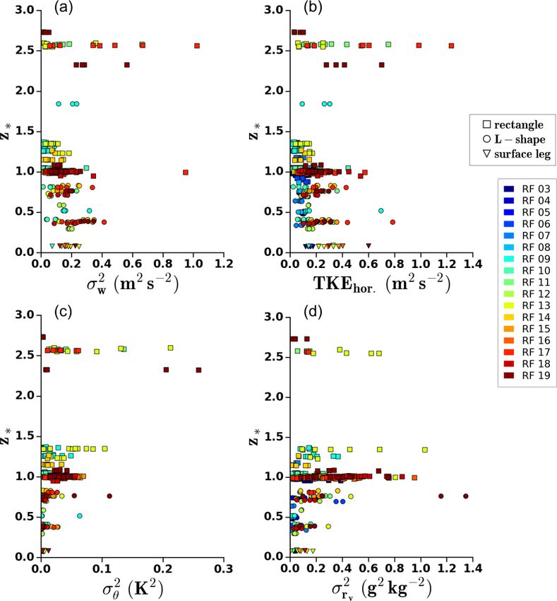
3386                                                                P.-E. Brilouet et al.: The EUREC4 A ATR 42 turbulence dataset

Figure 7. Comparison of LI-COR and KH20 signals on a leg flown at z ∼ 600 m on 13 February 2020 (RF19): (a) time series of water
vapor mixing ratio fluctuations from the LI-COR (in yellow) and from the KH20 (in blue). (b) Associated normalized energy density spectra.
Smoothed spectra are indicated by thick solid lines.

Figure 8. Humidity variances computed on 5 min segments for all the flights RF03 to RF19: (a) from the KH20 signals versus the LI-COR
signals and (b) from the KH20 signals versus the LI-COR signal corrected for noise. (c) Moisture flux from the KH20 signal versus from
the LI-COR signal for flights RF09 to RF19. The symbols correspond to the altitude of the leg. The dark green markers refer to legs with a
good-quality calibration of humidity for both sensors. Bright green markers refer to legs with a good-quality calibration of humidity for the
KH20 sensor only. The yellow–green markers refer to legs with a good-quality calibration of humidity for the LI-COR sensor only. Finally,
the bright pink markers correspond to the rest of the legs.

   As a result of this analysis, the KH20 sensor is primar-              adapted for taking account of uncorrelated noise (Lenschow
ily used for turbulence moment estimates and analysis of the             et al., 2000, 2012), since the autocovariance at zero lag is
fine-scale processes. But in the case of strong failure of this          equal to the variance of the signal plus the variance of the
sensor, the LI-COR is used as an alternative for the covari-             white noise. Here, we found that using the fifth lag was more
ance estimates. The variances of the LI-COR were corrected               appropriate due to slightly correlated noise and the need to
for noise (Fig. 8b) by using the value of the autocovariance             find a best compromise. This means that we lose the ampli-
function of moisture fluctuations at the fifth lag as an esti-           tude of the fluctuations of scales smaller than 20 m.
mate of the variance. The use of the first lag is common and

Earth Syst. Sci. Data, 13, 3379–3398, 2021                                                https://doi.org/10.5194/essd-13-3379-2021
P.-E. Brilouet et al.: The EUREC4 A ATR 42 turbulence dataset                                                                    3387

                                                                      5   Qualification of the fast temperature sensors

                                                                      On board the SAFIRE ATR 42, the temperature was mea-
                                                                      sured by two sensors: a Rosemount probe and a fine wire.
                                                                      The typical and reference Rosemount temperature probe
                                                                      showed some issues during the field campaign, including
                                                                      spurious negative spikes that were not visible on the fine wire
                                                                      sensor. Those were not easily explained but are supposed to
                                                                      be inherent to the sensor itself. Rarely, large noise could also
                                                                      appear locally in the presence of cloud droplets. The hous-
                                                                      ing of the Rosemount probe makes it difficult for the cloud
                                                                      droplets to penetrate the probe and to reach the sensor. How-
                                                                      ever, should a droplet reach the sensor, it takes more time to
                                                                      dry out. In contrast, the fine wire is more exposed, but it re-
Figure 9. Definition of a combined flag for the humidity, depending
                                                                      covers quickly. A usual weakness of the fine wire is its ability
on the KH20 and the LI-COR sensor quality flags. The number of
                                                                      to break with shocks, in particular during takeoff or landing.
segments and the associated percentage for each category of the
combined flag are indicated in the boxes on the right. It refers to   During EUREC4 A, the fine wires did not break and turned
flights RF03 to RF19 for the short legs.                              out to provide a better fine-scale signal than the Rosemount
                                                                      probe.
                                                                         The two fine wires were installed starting with flight RF09
                                                                      and calibrated with the Rosemount probe at 1 Hz for each
                                                                      flight. Both fine wires were consistent with the other, but one
                                                                      showed some noise that the other did not show at all. We
   We found that, generally, the KH20 sensor encountered is-          consider only the latter here. We considered this measure-
sues in legs close to the surface due to sea salt. This is clearly    ment non-absolute and used it only for the study of temper-
shown in Fig. 8c, where the legs with a green flag for LI-            ature fluctuations. We calibrated the fine wire with the raw
COR only (yellow–green) all show larger covariances with              impact temperature of the Rosemount probe temperature as
LI-COR. In contrast, the LI-COR had more difficulties when            a reference, with one calibration per flight. The regression
the SAFIRE ATR 42 was crossing clouds or even rain dur-               slope was very close to 1 (1.07 on average, with a standard
ing the “R” legs, while the KH20 behaved much better in               deviation of 1.2 % over the 11 flights concerned). The most
those wet conditions. Indeed, in Fig. 8c, all the legs associ-        significant variability was found in the offset (coordinate at
ated with a green flag for KH20 only show larger covariances          the origin of the regression line), which varied between −4.6
with KH20 than for LI-COR.                                            and −1.9 ◦ C, with a standard deviation of 2.6 ◦ C. This vari-
   In order to obtain the best estimate of the turbulent mo-          ation may be explained by the fine wire resistance varying
ments and fluctuations for each leg, they have been calcu-            with time due to oxidation. From this calibration and due to
lated using either one sensor or the other depending on their         the incertitude of the housing features and recovery factor,
respective flags, with priority given to the KH20 sensor. This        we applied the same recovery factor of the Rosemount (0.98)
results in the definition of a combined flag as illustrated in        to retrieve the static temperature from the impact tempera-
Fig. 9. In total, over the 535 5 min segments, 241 segments           ture. Those results were similar to those found in the analysis
are based on the KH20 with a green flag (green combined               of Baehr et al. (2002) for the same type of fine wire and the
flag), 113 are based on the LI-COR with a green flag as an al-        same antenna.
ternate (yellow combined flag), 153 are based on the KH20 or             Figure 10a shows a time series of the temperature fluctu-
the LI-COR with a yellow flag (orange combined flag), and             ations derived from each sensor during a subcloud layer leg
28 are unusable (red combined flag). Therefore, the calcu-            of RF19. The spikes of the Rosemount temperature probe
lation of the turbulent moments associated with humidity is           signal were particularly numerous in this example. The com-
trustworthy for the green and yellow combined flags. Orange           parison also reveals the shorter time response of the fine wire
flags should preferably be avoided, and red flags are automat-        and its better ability to catch the small-scale variability. This
ically invalidated. Finally, although the confidence in the cal-      is confirmed by the comparison of the spectra (in Fig. 10b),
culation of turbulent moments for the yellow flag is good, the        which shows how the fine wire temperature density energy
use of LI-COR fluctuations for studying fine-scale processes          spectrum (multiplied by the frequency) better follows the ex-
(e.g., with spectral analysis or probability density functions)       pected −2/3 slope in the inertial subrange.
should be avoided, as shown in Sect. 4.2. The KH20 sensor                The covariance between temperature and moisture is fur-
should be preferred because of its better description of the          ther evidence of the larger relevance of the fine wire signal
expected spectrum in the inertial range and its better record-        (Fig. 11). Temperature and moisture fluctuations are often
ing of the amplitude and the distribution of the fluctuations.        well correlated: for example, an intrusion of air from above

https://doi.org/10.5194/essd-13-3379-2021                                            Earth Syst. Sci. Data, 13, 3379–3398, 2021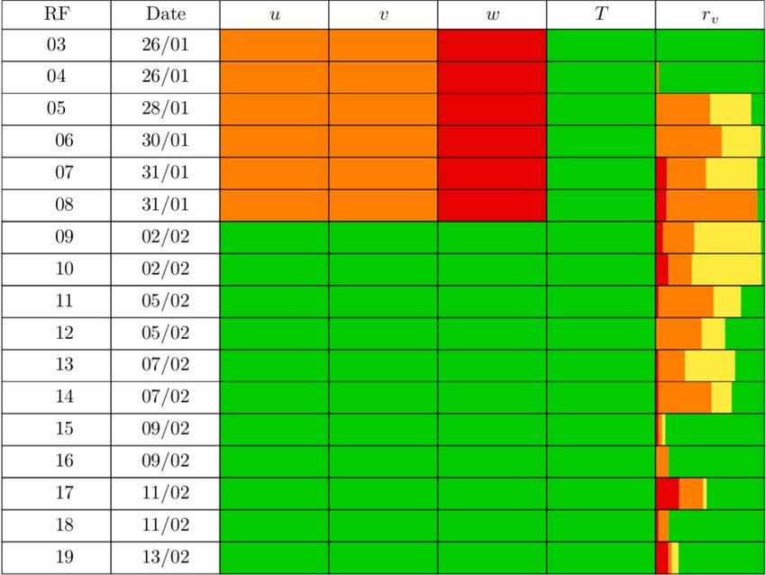
3388                                                              P.-E. Brilouet et al.: The EUREC4 A ATR 42 turbulence dataset

Figure 10. (a) Time series of the temperature fluctuations measured by the Rosemount probe (in red) and by the fine wire (in green) during
a subcloud layer leg of RF19. (b) Corresponding density energy spectrum.

is associated with a drier and warmer structure (negative and
positive fluctuations of moisture and temperature, respec-
tively). Figure 11 shows that this correlation is higher when
the temperature is measured by the fine wire than when it
is measured by the Rosemount probe. It is partly explained
by the fact that the temperature variance is larger with the
fine wire, but also because the fine wire tracks the fine-scale
fluctuations of temperature better than the Rosemount probe.
For these reasons, the fine wire temperature signal was cho-
sen during EUREC4 A for the best estimate of the turbulent
moments and fluctuations. The Rosemount probe tempera-
ture was used as a spare during the first part of the campaign
and during a few R legs of RF17 and RF19 when the fine
wire sensor was heavily impacted by cloud droplets. A green
flag was associated with the fine wire use and a yellow flag
with the use of the Rosemount probe.

6   Computation of turbulence moments and
                                                                       Figure 11. Comparison of the covariance of temperature and mois-
    associated errors
                                                                       ture obtained when using the Rosemount probe temperature (y axis)
                                                                       and the fine wire temperature (x axis). In both cases, the calculation
After control and calibration, the 25 Hz fluctuations are used
                                                                       is based on the moisture fluctuations associated with a green flag.
to compute the turbulence moments and other characteristics
of the MABL turbulence. The turbulent moments or charac-
teristics evaluated for each leg are listed in Table 2.
   Only stabilized legs are considered for the turbulence data         varying flight attitude and speed. Moreover, to obtain a ho-
processing due to the increase in errors in basic measure-             mogeneous statistical ensemble of turbulent moments associ-
ments during turns or more generally during phases with                ated with random and systematic error estimates, the straight

Earth Syst. Sci. Data, 13, 3379–3398, 2021                                               https://doi.org/10.5194/essd-13-3379-2021
P.-E. Brilouet et al.: The EUREC4 A ATR 42 turbulence dataset 3389
Table 2. List of turbulent parameters calculated over each segment, their standard nomenclature and their names in the NetCDF files.
General characteristics
Start, end, central time ti , tf , t time_start, time_end, time
Start, end, central position lati , loni , latf , lonf , lat, lon lat_start, lon_start, lat_end, lon_end, lat, lon
duration T duration
Mean heading THDG MEAN_THDG
Mean true airspeed TAS MEAN_TAS
Mean ground velocity GS MEAN_GS
Mean height above the sea z alt
Mean pressure P MEAN_P
Mean static temperature Ts MEAN_TS
Mean air density ρa MEAN_RHO_A
Calibration information
Quality flag for humidity signal QC_MR
Humidity sensor used HUM_SENSOR
Quality flag for temperature signal QC_T
Temperature sensor TEMP_SENSOR
First-order moments
Mean wind FF, DD MEAN_WSPD, MEAN_WDIR
Mean potential temperature θ MEAN_THETA
Mean water vapor mixing ratio rv MEAN_MR
Second-order moments, filtering ratios and associated errors
Wind components variance u0 2 , R , s VAR_U, RATIO_VAR_U, ERR_S_VAR_U
u0 2 u0 2
v0 2 , R , s 2 VAR_V, RATIO_VAR_V, ERR_S_VAR_V
v0 2 v0
0 2
w , R 0 2 , s 2 VAR_W, RATIO_VAR_W, ERR_S_VAR_W
w w0
Turbulent kinetic energy e, Re TKE, RATIO_TKE
Turbulent kinetic energy dissipation rate EPSILON_TKE
Potential temperature variance θ 02, R , s VAR_T, RATIO_VAR_T, ERR_S_VAR_T
θ 02 θ02
Water vapor mixing ratio variance r 0 2v , R , s VAR_MR, RATIO_VAR_MR, ERR_S_VAR_MR
r 0 2v r 0 2v
Covariances with the vertical velocity w 0 u0 , Rw0 u0 , s , r COVAR_WU, RATIO_COVAR_WU, ERR_S_COVAR_WU,
w 0 u0 w 0 u0
ERR_R_COVAR_WU
w 0 v 0 , Rw0 v 0 , s , r COVAR_WV, RATIO_COVAR_WV, ERR_S_COVAR_WV,
w0 v 0 w0 v 0
ERR_R_COVAR_WV
w 0 θ 0 , Rw0 θ 0 , s , r COVAR_WT, RATIO_COVAR_WT, ERR_S_COVAR_WT,
w0 θ 0 w0 θ 0
ERR_R_COVAR_WT
w 0 r 0 v , Rw0 r 0 , s , r COVAR_WMR, RATIO_COVAR_WMR,
v w 0 rv0 w 0 rv0
ERR_S_COVAR_WMR, ERR_R_COVAR_WMR
Third-order moments and filtering ratios
u0 3 , R M3_U, RATIO_M3_U
Wind component third-order moment u0 3
v0 3 , R M3_V, RATIO_M3_V
v0 3
w0 3 , R 0 3 M3_W, RATIO_M3_W
w
Potential temperature third-order moment θ 03, R M3_THETA, RATIO_M3_THETA
θ 03
Water vapor mixing ratio third-order moment r 0 3v , R M3_MR, RATIO_M3_MR
r 0 3v
Skewness of each thermodynamic variables Su , Sv , Sw , Sθ , Srv SKEW_U, SKEW_V, SKEW_W, SKEW_T, SKEW_MR
Characteristic length scales
Vertical velocity spectrum peak wavelength λw LAMBDA_W
Integral length scales Lw , Lwu , Lwv , Lwθ , Lwrv L_W, L_WU, L_WV, L_WT, L_WMR
https://doi.org/10.5194/essd-13-3379-2021 Earth Syst. Sci. Data, 13, 3379–3398, 20213390 P.-E. Brilouet et al.: The EUREC4 A ATR 42 turbulence dataset
two variables x and y is defined as
ZT
1
x0y0 = x 0 (t)y 0 (t)dt, (1)
T
0
where T is the duration of the leg. From the variances of u,
v and w, the turbulent kinetic energy (TKE) is calculated as
TKE = 12 (σu2 + σv2 + σw2 ). Third-order turbulent moments are
also computed, enabling the calculation of the skewness of a
Figure 12. Schematic view of the segmentation of stabilized legs variable x:
into segments of equal duration and length: 30 km, 5 min long seg-
ments (“short legs”, in red) and 60 km, 10 min long segments (“long x03
Sx = 3/2 . (2)
legs”, in purple). Also reported are the “longest legs” (in green),
x02
which are the longest stabilized segments in one direction.
For both second-order and third-order moments, the ratio, de-
noted as R in Table 2, between the moment obtained without
high-pass filtering (fluctuations obtained only by detrending
the original series) and that obtained after high-pass filtering
horizontal legs are divided into segments of equal duration
is computed. This index provides information about the sta-
and length. Two types of segments are considered (Fig. 12):
tionarity and homogeneity of a sample. For a perfectly homo-
segments of 60 km and 10 min (referred to as “long legs”),
geneous and stationary sample with no impact of mesoscale
which correspond to the length of an “L” branch, and seg-
or sub-mesoscale structures, this ratio should theoretically be
ments of 30 km and 5 min (referred to as “short legs”). As
equal to 1. It is often close to 1 for vertical velocity variance
suggested by Lenschow et al. (1994), 30 km long segments
but can be much larger for other variables and for covari-
are a good compromise, as they are long enough to sam-
ances.
ple the structures which dominate the turbulent exchanges
Characteristic length scales suitable to describe the tur-
and short enough to explore the spatial variability from one
bulence field are also computed, such as the wavelength of
leg to the other. Note that the short legs are occasionally ad-
the vertical velocity spectrum peak or integral length scales.
justed within the subcloud layer (during L legs) to avoid wa-
The length scale of the maximum spectral density energy of
ter droplets (two segments of that kind).
vertical velocity is obtained by fitting an analytical spectrum
For each segment, the turbulent moments are calculated f S0
of the form f S(f ) = , where f is the frequency,
f 5/3
from two types of fluctuations time series: detrended series or 1+1.5 f0
high-pass-filtered series, with a cutoff frequency of 0.018 Hz and S0 and f0 are fitted to the observed vertical velocity spec-
(about 5 km wavelength). This filter is meant to remove the tra (Lambert and Durand, 1999; Attie et al., 1999). Depend-
contribution of mesoscale features. The cutoff wavelength is ing on purpose, more complex analytical spectra may be used
chosen based on the co-spectra of the vertical velocity with to estimate the wavelength of maximum spectral energy (see,
all other variables (temperature, humidity, horizontal compo- e.g., Kristensen et al., 1989; Lothon et al., 2009 or Brilouet et
nents) so that all turbulent scales contributing to the covari- al., 2017) and other definitions (e.g., Pino et al., 2006). This
ance are taken into account. one is chosen for the sake of simplicity.
Figure 13 shows an example of the filtered time series of The integral length scale of a variable x is estimated as the
five variables: w 0 , θ 0 , rv0 , u0L and vT0 . The prime symbol in- integral of the normalized autocorrelation function from zero
dicates a fluctuation relative to the mean value. Here u0L and lag (τ = 0) to the first zero (τ0 ) of the function (Lenschow et
vT0 are respectively the longitudinal and lateral fluctuations of al., 1994):
the horizontal wind relative to the mean wind over the con-
sidered leg. The longitudinal and lateral fluctuations of the Zτ0
1
horizontal wind relative to the aircraft, u0x and vy0 , are also Lx = x 0 (t)x 0 (t + τ )dτ. (3)
calculated and made available in the dataset, as are the fluc- x02 0
tuations of eastward and northward components. The use of
one or the other referential depends on the purpose of the The turbulent kinetic energy dissipation rate (ε) is esti-
turbulence data analysis. In all three referentials, the vertical mated from the vertical velocity energy spectrum Sw in the
velocity is taken positive upward, and the referential systems inertial subrange (Lambert and Durand, 1998) based on the
are direct and orthogonal. Kolmogorov formulations: Sw (k) = 43 αε2/3 k −5/3 , where k is
2π
The second- and third-order turbulent moments are com- the wavenumber (k = TAS f ) and α is the Kolmogorov con-
puted with the eddy correlation method. The covariance of stant, taken as α = 0.52 (Fairall and Larsen, 1986).
Earth Syst. Sci. Data, 13, 3379–3398, 2021 https://doi.org/10.5194/essd-13-3379-2021P.-E. Brilouet et al.: The EUREC4 A ATR 42 turbulence dataset 3391
Figure 13. Time series of the filtered fluctuations of (a) vertical velocity, (b) wind velocity component longitudinal to the wind, (c) wind
velocity component transverse to the wind, (d) potential temperature and (e) water vapor mixing ratio during a leg flown at z ∼ 275 m on
13 February 2020 (RF19).
The reliability and accuracy of the observed turbulent mo- of the high-pass-filtered series (Ffil ):
ment estimates can be assessed based on sampling and fil- Fdet − Ffil
tering conditions. As introduced by Lenschow et al. (1994), s = . (4)
Fdet
using high-pass-filtered and finite-length samples generates
an error which can be decomposed into two contributions: The random error is generated by the finite length of the sam-
a systematic error (s ) and a random error (r ). The system- ple and is therefore inherent in the measurement and cannot
atic error reflects the loss of information due to the high-pass be removed. For a covariance between two variables x and y,
filtering and can be estimated as the difference between the the associated random error can be estimated by
s
covariance of the detrended series (Fdet ) and the covariance
r
2Lxy 1
r = 1+ 2 , (5)
L rxy
https://doi.org/10.5194/essd-13-3379-2021 Earth Syst. Sci. Data, 13, 3379–3398, 20213392 P.-E. Brilouet et al.: The EUREC4 A ATR 42 turbulence dataset
where Lxy is the integral length scale of x 0 y 0 , L the length of
the leg, and rxy the correlation coefficient between x and y.
7 Available dataset
The dataset includes two kinds of data.
1. Moments. The turbulent moments are calculated over
each segment. The data are stored in NetCDF files
(with one file per flight) for the three sets of short
(30 km) and long (60 km) segments as well as over the
longest possible segments of stabilized legs. However,
one should note that these “longest” segments have dif-
ferent lengths that range from 60 to 125 km.
2. Fluctuations. The time series of fluctuations over each
segment, filtered and detrended only, are made available
to enable specific analyses or estimates of the turbulent Figure 14. Quality flags associated with the turbulent data for
each SAFIRE ATR 42 flight during the campaign. The data qual-
moments through an alternative approach. There is one
ity increases from red (poor quality) to orange, yellow and green
NetCDF file per segment and per flight. (high quality). For moisture and temperature, the flag is the com-
Note that the fluctuations and moments over the longest bined flag described in Sects. 4 and 5, considering the short legs of
L3 data.
possible segments are also made available, even if this last
set is composed of segments of different lengths (from 60
to 125 km). It enables any user to work on the longest se-
ries of calibrated fluctuations for the entire stabilized legs. Of As an illustration of the dataset, Fig. 15 shows an overview
course, moments of R legs of 125 km are likely still more het- of the vertical profiles of variances for the entire field ex-
erogeneous and should be considered only in specific strict periment (RF03 to RF19). The profiles are normalized by
conditions. the lifting condensation level (LCL), estimated here as the
For both the turbulent fluctuations and turbulent moments, flight altitude of the rectangle at the cloud base minus 50 m.
two levels of data processing are considered. Overall, the turbulence is weak in the subcloud layer during
EUREC4 A. As expected in an MABL, the variance of verti-
– Level 2. All files of turbulent moments and fluctuations cal velocity is maximum within the first half of the subcloud
are calculated for each sensor of temperature and hu- layer, and the variance of the horizontal wind is larger near
midity. the sea surface. The variances of temperature and moisture
– Level 3 (or “best estimates’). Turbulent moments and are maximum near cloud base and the entrainment layer, and
fluctuations are derived from the sensors (or their com- they are minimum close to the surface. The very large scat-
bination) that have the best quality flags for the leg un- ter of the turbulent moments on R legs flown around cloud
der consideration (the flags are described in Sects. 4 and base likely reflects the large heterogeneity of the samples,
5); for each leg, they are considered as the best estimates related to the crossing of clouds and the mix of air masses
of moments and fluctuations given the available instru- of very different origins and characteristics (including non-
mentation. turbulent air masses). Over these legs, the moments need to
be taken with caution because their definition assumes a ho-
Table 3 explains the file nomenclature using Fig. 12 for mogeneous sample, which is a condition rarely met at cloud
the naming of each segment. For each flight, a YAML file is base.
provided together with the dataset that defines the start and Finally, Fig. 16 shows, for flights RF09 to RF19, the ver-
end times of each flight segment. tical profiles of the covariance of the vertical velocity with
Figure 14 summarizes the availability and the quality of temperature (Fig. 16a) or moisture (Fig. 16b), as well as
the high-rate data associated with each key variable. Based their corresponding systematic and random errors. Around
on the quality control described in Sects. 5 and 6 for temper- cloud base (z∗ ∼ 1), the random and systematic errors are
ature and moisture, it displays the proportion of legs within very large. This is explained by the large heterogeneity of
each flight that are associated with a green flag, as established the samples at this level and indicates that the vertical flux
on the basis of the L3 “short legs” dataset. This table shows estimates are mostly relevant below cloud base.
how the quality of the measurements improved in the sec- The sensible heat flux is very small near the surface (likely
ond phase of the field campaign (from RF09), with the best due to the small air–sea temperature difference) and changes
quality and availability achieved from RF15 onwards. sign with height, consistent with the entrainment near cloud
Earth Syst. Sci. Data, 13, 3379–3398, 2021 https://doi.org/10.5194/essd-13-3379-2021P.-E. Brilouet et al.: The EUREC4 A ATR 42 turbulence dataset 3393
Table 3. File nomenclature. YYYYMMDD corresponds to the flight date (e.g., 20200202), NN to the flight number (e.g., 09), LEG to the
segment identifier (e.g., R2B or l2c) and LEVEL to the level of data processing (L2 or L3).
Moments
30 km segments EUREC4A_ATR_turbulence_moments_YYYYMMDD_RFNN_shortlegs_LEVEL_version.nc
60 km segments EUREC4A_ATR_turbulence_moments_YYYYMMDD_RFNN_longlegs_LEVEL_version.nc
Longest segments EUREC4A_ATR_turbulence_moments_YYYYMMDD_RFNN_longestlegs_LEVEL_version.nc
Fluctuations
30 km segments EUREC4A_ATR_turbulence_fluctuations_YYYYMMDD_RFNN_textitLEG_LEVEL_version.nc
60 km segments EUREC4A_ATR_turbulence_fluctuations_YYYYMMDD_RFNN_textitLEG_LEVEL_version.nc
Longest segments EUREC4A_ATR_turbulence_fluctuations_YYYYMMDD_RFNN_textitLEG_LEVEL_version.nc
Figure 15. Normalized vertical profiles of the variance of (a) vertical velocity, (b) horizontal turbulent kinetic energy, (c) temperature and
(d) water vapor mixing ratio. Flight numbers are indicated in the top right box. For the water vapor mixing ratio, only the legs with a green
or a yellow combined flag have been considered. The normalized altitude z∗ is defined by z/LCL with LCL, the lifting condensation level.
base. The moisture flux is more significant, with a large value small fluctuations observed, resulting in very weak fluxes.
near the surface and an overall decrease in the flux with Inside the MABL, the random error increases with altitude,
height. partly related to the growth of the turbulent eddies. The pro-
For both the heat flux and the moisture flux, the system- files are similar to those found by Brilouet et al. (2017) dur-
atic error can be particularly large. This is largely due to the ing the HyMeX campaign over the Mediterranean Sea, which
https://doi.org/10.5194/essd-13-3379-2021 Earth Syst. Sci. Data, 13, 3379–3398, 20213394 P.-E. Brilouet et al.: The EUREC4 A ATR 42 turbulence dataset Figure 16. Normalized vertical profiles of (a) the heat flux, (b) the moisture flux, systematic error (c) for the heat flux, systematic error (d) for the moisture flux, random error (e) for the heat flux and random error (f) for the moisture flux. Flight numbers are indicated in the top right box. The normalized altitude z∗ is defined by z/LCL with LCL, the lifting condensation level. Earth Syst. Sci. Data, 13, 3379–3398, 2021 https://doi.org/10.5194/essd-13-3379-2021
P.-E. Brilouet et al.: The EUREC4 A ATR 42 turbulence dataset                                                                      3395

took place in much stronger wind conditions than here. Like             The variance and covariance estimates are not affected
in HyMeX, we find larger errors in the heat flux than in the            by these limitations, but we recommend that the spec-
moisture flux due to the more significant moisture fluctua-             tral or distribution analyses of the turbulent fluctuations
tions.                                                                  primarily use the data from the KH20 moisture sensor
   On the R legs above the MABL, the errors display a wide              and from the fine wire temperature sensor.
variability and potentially large values. This again reflects
the high heterogeneity of the samples and the influence of
the mesoscales at this height.
                                                                     – Owing to the weakness of the turbulent fluxes during
                                                                       EUREC4 A, the turbulent moment estimates are asso-
8    Data availability                                                 ciated with large systematic and random errors. This,
                                                                       added to the limited vertical sampling of the MABL,
The dataset is available at https://eurec4a.aeris-data.fr/             suggests that extrapolating sea surface turbulent fluxes
(last access: 6 July 2021, Lothon and Brilouet, 2020,                  from this dataset would not be accurate.
https://doi.org/10.25326/128).

                                                                      Despite these issues and the technical difficulties
9    Conclusions                                                   encountered at the beginning of the campaign, a rich and
                                                                   quality-controlled dataset has been produced based on the
This paper presents the EUREC4 A turbulent dataset that has
                                                                   high-rate measurements of the SAFIRE ATR 42 that will
been produced based on the high-rate in situ measurements
                                                                   make it possible to study the turbulence of the MABL during
of wind, temperature and moisture from the SAFIRE ATR
                                                                   EUREC4 A.
42. It explains the data processing strategies, the calibration
                                                                      These data will be used to characterize the structure and
methodologies, the procedures of quality control applied to
                                                                   the variability of the subcloud layer and the level of organi-
the 25 Hz temperature and moisture measurements, and the
                                                                   zation encountered underneath the clouds. Used jointly with
methods used to estimate the turbulent moments and their
                                                                   the other EUREC4 A datasets from aircraft, balloons or un-
associated errors.
                                                                   manned aerial vehicles, they will help to decipher the nature
   The redundancy of temperature and moisture sensors on
                                                                   of cloud–circulation interactions and to identify the roots of
board the aircraft enabled us to overcome the failure of one or
                                                                   the shallow convective organization. They will also help eval-
the other sensor and to optimize the data processing. All tur-
                                                                   uate the ability of large-eddy simulations to predict the char-
bulent moments and time series of turbulent fluctuations are
                                                                   acteristics of turbulence within the subcloud layer of trade-
associated with some information about the sensor(s) from
                                                                   wind regimes for a range of large-scale conditions.
which they are derived, plus a quality flag. These data con-
stitute the Level-2 dataset. In addition, a Level-3 dataset pro-
vides an ensemble of best estimates of the turbulent moments       Author contributions. PEB and ML designed the data processing
and fluctuations over each stabilized leg of the SAFIRE ATR        strategy, processed and analyzed the data, and wrote the paper. They
42 flights.                                                        participated in the SAFIRE ATR 42 flight coordination on board
   Considering our analysis of the data as well as the flight      during the field experiment.
strategy and conditions, we make the following remarks and            JCE and PR processed the initial SAFIRE data to generate the
recommendations to future users of this dataset.                   25 Hz data and participated in the data quality control.
                                                                      JL was the SAFIRE instrumentalist mostly involved in the adap-
    – The data collected at cloud base over the R legs or seg-     tation of the KH20 sensor; he monitored and maintained the sensors
      ments should be used with great caution. First, the pres-    during the field experiment.
      ence of cloud droplets or rain may affect the perfor-           HB, GV, TP and JL are instrumentalist experts on the SAFIRE
      mance of the high-rate sensors. In addition, at this level   ATR 42, who contributed to preparation for the field campaign re-
      the aircraft probes very contrasting air masses, includ-     garding the airborne instrumentation.
      ing clouds and cloud-free air originating from the sub-         TJ, FP, CL and MC were responsible for the data acquisition on
                                                                   board and the preliminary data processing.
      cloud layer or entrained from above. The large hetero-
                                                                      PM, TC and LG contributed with SAFIRE instrumentalists to the
      geneity of the samples makes the calculation of turbu-       initial adaptation of the KH20 sensor to the aircraft at the very start
      lent moments quite uncertain around cloud base. How-         of the instrumental project.
      ever, the turbulent fluctuations remain relevant and can        SB is the co-lead coordinator of the EUREC4 A campaign and the
      be used for specific analyses such as conditional sam-       lead scientific coordinator of the SAFIRE ATR operations. She par-
      pling, object approaches or case studies.                    ticipated in the flights and in the monitoring of the measurements.
                                                                   She participated in the discussions on data analysis and edited the
    – The moisture fluctuations measured by the LI-COR sen-        paper.
      sor and the temperature fluctuations measured by the            JD and ML were co-coordinators of the SAFIRE ATR 42 opera-
      Rosemount probe exhibit limitations at very fine scales.     tions during the EUREC4 A campaign.

https://doi.org/10.5194/essd-13-3379-2021                                           Earth Syst. Sci. Data, 13, 3379–3398, 2021
You can also read