Unsupervised classification of vertical profiles of dual polarization radar variables
←
→
Page content transcription
If your browser does not render page correctly, please read the page content below
Atmos. Meas. Tech., 13, 1227–1241, 2020
https://doi.org/10.5194/amt-13-1227-2020
© Author(s) 2020. This work is distributed under
the Creative Commons Attribution 4.0 License.

Unsupervised classification of vertical profiles of dual
polarization radar variables
Jussi Tiira1 and Dmitri Moisseev1,2
1 Institute for Atmospheric and Earth System Research/Physics, Faculty of Science, University of Helsinki, Helsinki, Finland
2 Finnish   Meteorological Institute, Helsinki, Finland

Correspondence: Jussi Tiira (jussi.tiira@helsinki.fi)

Received: 9 August 2019 – Discussion started: 20 August 2019
Revised: 21 January 2020 – Accepted: 2 February 2020 – Published: 13 March 2020

Abstract. Vertical profiles of polarimetric radar variables can     itation rate (von Lerber et al., 2017), identification of dan-
be used to identify fingerprints of snow growth processes. In       gerous weather conditions, etc. To address these challenges,
order to systematically study such manifestations of precipi-       advances in identifying and documenting the processes that
tation processes, we have developed an unsupervised classi-         take place in ice clouds are needed.
fication method. The method is based on k-means clustering             There are several pathways by which ice particles grow,
of vertical profiles of polarimetric radar variables, namely        such as vapor deposition, aggregation and riming. Occur-
reflectivity, differential reflectivity and specific differential   rence of these processes depends on environmental condi-
phase. For rain events, the classification is applied to radar      tions. Interpretation of radar observations is based on our un-
profiles truncated at the melting layer top. For the snowfall       derstanding of the link between microphysical and scattering
cases, the surface air temperature is used as an additional in-     properties of hydrometeors. By identifying particle types in
put parameter. The proposed unsupervised classification was         observations, we may conclude what processes took place.
applied to 3.5 years of data collected by the Finnish Me-           Currently, dual-polarization radar observations are used in
teorological Institute Ikaalinen radar. The vertical profiles       fuzzy logic classification to identify the dominant hydrom-
of radar variables were computed above the University of            eteor type present in a radar volume (e.g., Chandrasekar
Helsinki Hyytiälä station, located 64 km east of the radar.         et al., 2013; Thompson et al., 2014). Such methods work very
Using these data, we show that the profiles of radar variables      well for classification of hydrometeors of summer precipita-
can be grouped into 10 and 16 classes for rainfall and snow-        tions and some features of winter precipitation types. The
fall events, respectively. These classes seem to capture most       main challenge is the lack of distinction in dual-polarization
important snow growth and ice cloud processes. Using this           radar variables between some ice particle habits. For exam-
classification, the main features of the precipitation forma-       ple, large low-density aggregates and graupel may have sim-
tion processes, as observed in Finland, are presented.              ilar radar characteristics. Furthermore, these methods per-
                                                                    form classification on radar volume by volume basis, with-
                                                                    out taking into account surrounding observations. Recently,
                                                                    a modification for the hydrometeor classifiers was proposed
1   Introduction                                                    to make the algorithms aware of the surroundings by in-
                                                                    corporating measurements from neighboring radar volumes
Globally, the majority of precipitation during both winter          (Bechini and Chandrasekar, 2015; Grazioli et al., 2015b).
and summer originates from ice clouds (Field and Heyms-             This step has greatly improved classification robustness, but
field, 2015). At higher latitudes winter precipitation occurs       it aims to identify particle types instead of fingerprints of mi-
in the form of snow, which can have a dramatic impact on            crophysical processes.
human life (Juga et al., 2012). There are a number of chal-            In the past 10 years, a number of studies reported sig-
lenges in remote sensing of winter precipitation or ice clouds,     natures of ice growth processes in dual-polarization radar
i.e., quantitative estimation of ice water content or precip-

Published by Copernicus Publications on behalf of the European Geosciences Union.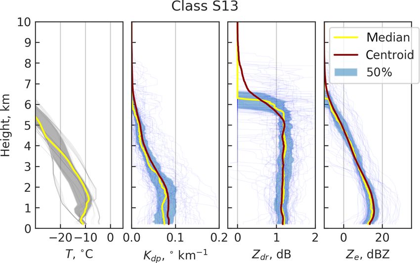
1228                                                J. Tiira and D. Moisseev: Unsupervised classification of vertical profiles

observations. Kennedy and Rutledge (2011) have reported            Sect. 3. Section 4 is dedicated to the analysis and interpreta-
bands of increased values of specific differential phase, Kdp ,    tion of the classification results and Sect. 5 presents the con-
and differential reflectivity, ZDR , in Colorado snowstorms.       clusions.
These bands took place at altitudes where ambient air tem-
perature was around −15 ◦ C and their occurrence was at-
tributed to growth of dendritic crystals. Andrić et al. (2013)    2     Data
have implemented a simple steady-state single-column snow
growth model to explain the main features of the bands. It         In this study, we use vertical profiles of polarimetric radar
was also observed that the occurrence of Kdp bands can be          observables of precipitation over the Hyytiälä forestry sta-
linked to heavier surface precipitation (Kennedy and Rut-          tion in Juupajoki, Finland, collected using Ikaalinen weather
ledge, 2011; Bechini et al., 2013). Moisseev et al. (2015)         radar, hereafter IKA. The radar is located 64 km west from
have advocated that the Kdp bands occur only in precipita-         the station. The measurements were performed between
tion systems with high enough cloud-top heights, where a           January 2014 and May 2017, partly during the Biogenic
large number of ice crystals can be generated by either het-       Aerosols – Effects on Clouds and Climate (BAECC; Petäjä
erogeneous or homogeneous ice nucleation. Using a larger           et al., 2016) field campaign which took place at the measure-
dataset, Griffin et al. (2018) have shown that the Kdp bands       ment site in 2014.
can be linked to formation of ice by homogeneous ice nucle-           The classification training material includes all precipita-
ation at cloud tops. Furthermore, it was shown that the Kdp        tion events from this period, where, after preprocessing (see
bands can be linked to onset of aggregation (Moisseev et al.,      Sect. 2.2), there were no major data quality problems identi-
2015), which tends to occur more frequently in environments        fied. Since synoptic conditions may be similar even in cases
with higher water vapor content (Schneebeli et al., 2013).         where there are gaps in observed precipitation, we define any
In addition to the above-listed studies, different aspects of      two precipitation events to be separate from each other if
these bands were presented by Trömel et al. (2014), Oue            a continuous gap in reflectivity between them exceeds 12 h.
et al. (2018), and Kumjian and Lombardo (2017). Besides            See Sect. 4 for more discussion. During the observation pe-
Kdp bands in the dendritic growth zone, several studies (e.g.,     riod, we identified 74 snow and 123 rain events that meet
Grazioli et al., 2015a; Sinclair et al., 2016; Kumjian et al.,     these conditions. Generally, the full temporal extent of an
2016; Giangrande et al., 2016) have reported Kdp observa-          event includes radar profiles in which precipitation has not
tions in the temperature region where Hallett–Mossop (H–           reached the ground. A list of the precipitation events is given
M; Hallett and Mossop, 1974) rime-splintering secondary            in the Supplement.
ice production takes place (Field et al., 2016). Sinclair et al.      In order to link features identified in vertical profiles of
(2016) have shown that such observations can be used to test       radar variables to precipitation processes, information on the
representation of the secondary ice production in numerical        ambient temperature is needed. For this purpose we use ver-
weather prediction models. Other dual-polarization observa-        tical profiles of temperature from the National Center for
tions that show notable features are high-ZDR regions sur-         Environmental Prediction (NCEP) Global Data Assimilation
rounding the cores of snow-generating cells (Kumjian et al.,       System (GDAS) output for Hyytiälä interpolated to match
2014) and at the top of ice clouds which can be linked to the      the temporal and vertical resolution of the vertical profiles of
presence of planar crystals and further to the presence of su-     radar variables used in this study. The original temporal res-
percooled liquid water, providing very favorable conditions        olution of the NCEP GDAS data over Hyytiälä is 3 h, and the
for their growth at these temperatures (Williams et al., 2015;     vertical resolution is 25 hPa between the 1000 and 900 hPa
Oue et al., 2016).                                                 levels and 50 hPa elsewhere.
   As presented above, the fingerprints of snow growth pro-
cesses can occur in the form of bands in stratiform clouds, ei-    2.1    Vertical profiles of dual-polarization radar
ther embedded in the precipitation or on top of a cloud, or in            observables
the form of convective generating cells. To identify and docu-
ment such features, a classification method that uses vertical     The radar profiles are extracted from IKA C-band radar range
profiles of dual-polarization radar observations can be used.      height indicator (RHI) measurements. IKA performs RHI
In this study, we have developed such an unsupervised classi-      scans directly towards Hyytiälä station every 15 min. The
fication method based on k-means clustering of vertical pro-       values of the radar profiles above Hyytiälä are estimated as
files of polarimetric radar variables, namely reflectivity, dif-   horizontal medians over a range of 1 km from the station.
ferential reflectivity and specific differential phase. The pro-   The medians are taken over constant altitudes using linear
posed classification is applied to 3.5 years of data collected     spatial interpolation between the rays. The target bin size of
with the Finnish Meteorological Institute Ikaalinen radar.         the height interpolation is 50 m.
   The paper is structured as follows. Section 2 describes po-        In this investigation, vertical profiles of equivalent reflec-
larimetric radar and temperature data and their preprocess-        tivity factor, Ze , differential reflectivity, ZDR , and specific
ing. The unsupervised classification method is presented in        differential phase, Kdp , are considered in the classification.

Atmos. Meas. Tech., 13, 1227–1241, 2020                                              www.atmos-meas-tech.net/13/1227/2020/
J. Tiira and D. Moisseev: Unsupervised classification of vertical profiles                                                    1229

The Kdp values were computed using the Maesaka et al.                    low), with chosen values of 2 and 0.3, respectively. The
(2012) method as implemented in the Python ARM Radar                     SciPy (version 1.3; Virtanen et al., 2020) implementa-
Toolkit (Py-ART; Helmus and Collis, 2016). The method                    tion of the peak detection algorithm1 is used here.
assumes that propagation differential phase, φDP , increases
monotonically with increasing range from the radar. In this          2. Median ML height, h̃ML , is computed as the weighted
study, we mainly focus on precipitation processes typically             median of the peak altitudes, hi , using the product of
occurring in stratiform precipitation, where negative Kdp is            peak absolute amplitude and HIML as weights. Peaks
not important. The Maesaka et al. (2012) algorithm should               above a chosen height threshold of hthresh = 4200 m are
be avoided when studying precipitation events with lightning            ignored in this step.
activity, where negative Kdp may occur due to electrifica-
tion (Caylor and Chandrasekar, 1996). Negative Kdp has also
been reported during events of conical graupel which have            3. Step 1 is run again, this time only considering data
been linked to observations of generating cells (Oue et al.,            within h̃ML ± 1hML with a chosen 1hML value of
2015). The total fraction of profiles analyzed in this study            1500 m. If multiple peaks exceed the threshold values
where conical graupel appear or which represent strong con-             within a profile, the one with the highest amplitude is
vective cells with a possibility for lightning activity is ex-          used.
pected to be marginal, as discussed further in Sect. 4.
                                                                       The ML top height hML,top is estimated as the altitude cor-
2.2     Radar data preprocessing                                    responding to the 0.3HIML upper contour of the peak. Peak
                                                                    prominence, H , is a measure of how much a peak stands out
Prior to training or using the polarimetric radar vertical pro-     from the surrounding baseline value and is defined as the dif-
file data for the classification, noise and clutter filtering is    ference between the peak value and its baseline. The base-
applied to the binned profiles, which is followed by normal-        line is the lowest contour line of the peak encircling it but
ization and smoothing. Additionally, there are different pre-       containing no higher peak (Virtanen et al., 2020).
processing procedures for rain and snow events that allow              It should be noted that in steps 2 and 3, the analysis height
ambient temperature to be taken into account in the classi-         is limited to reflect the climatology of temperature profiles
fication. This section describes the mentioned preprocessing        on the measurement site. In step 2, we assume the ML to
steps in more detail.                                               be always below hthresh , and in step 3 we expect melting
                                                                    layer height not to change more than 1hML during an event.
2.2.1    Profile truncation                                         Such use of domain knowledge allows more robust ML de-
                                                                    tection in situations where IML has high values elsewhere.
This paper focuses on identifying, characterizing and inves-
                                                                    This may occur in the dendritic growth layer (DGL), for ex-
tigating the frequencies of different types of vertical struc-
                                                                    ample, where the crystals can be pristine enough to cause a
tures of dual-polarization radar variables specifically from
                                                                    significant increase in ZDR and a decrease in ρ.
the perspective of detecting, documenting and studying ice
                                                                       Sensitivity of the retrieved hML,top is tested for small
processes. Therefore, before the classification, vertical pro-
                                                                    changes in peak detection parameters discarding inconsis-
files of radar variables are truncated at the top of the melting
                                                                    tent values. A moving window median threshold filter is ap-
layer (ML), if one is present. Cases where melting layer sig-
                                                                    plied on time series of hML,top in order to discard rapid high-
natures were not identified and surface air temperature was
                                                                    amplitude fluctuations caused by noise in ZDR , for example.
1 ◦ C or lower are placed in the snowfall category and inves-
                                                                    A rolling triangle mean with a window size of five profiles,
tigated separately.
                                                                    corresponding to 1 h, is used for smoothing. Finally, linear
   Following Wolfensberger et al. (2015), who have used gra-
                                                                    interpolation and constant extrapolation is applied to hML,top
dient detection on a combination of normalized ZH and ρhv
                                                                    on a per-precipitation-event basis to make the estimate con-
for ML detection, we combine ρhv and standardized Ze and
                                                                    tinuous. This robust, albeit fairly complex, procedure pro-
ZDR into a melting layer indicator:
                                                                    duces a smooth estimate for melting layer top height. The
IML = Ẑe ẐDR (1 − ρhv ).                                   (1)    results from the ML detection were analyzed manually and
                                                                    the events with errors were discarded. In 90 % of events in
   The same standardization of Ze and ZDR is used here as in        the original dataset, the ML was detected without errors.
classification, as described in Sect. 3.1. In this study, instead      The analysis of rain profiles is limited to a layer from
of gradient detection, we use peak detection on smoothed            1hmargin = 300 m to 10 km above hML,top . The purpose of
IML to find the ML. Peaks are defined as any sample whose           the margin 1hmargin is to prevent properties of the melting
direct neighbors have a smaller amplitude and are found in          layer from leaking to the clustering features. The truncation
three steps.                                                        described in this section has no effect on the height bin size.
  1. Peak detection is performed with thresholds for absolute
     peak amplitude and prominence (HIML , as described be-            1 Function scipy.signal.find_peaks.

www.atmos-meas-tech.net/13/1227/2020/                                                 Atmos. Meas. Tech., 13, 1227–1241, 2020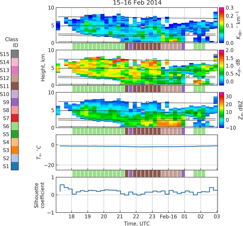
1230                                                         J. Tiira and D. Moisseev: Unsupervised classification of vertical profiles

Table 1. Standardization of radar variables, [a, b] → [0, 1].               3.1   Feature extraction

                              Rainfall        Snowfall
                               a         b     a         b                  The vertical resolution of the interpolated data is 50 m with
                                                                            bins from 200 m to 10 km altitude for snow events and from
           Ze , dBZ         −10       38     −10      34                    300 m to 10 km above the melting layer top for rain events.
           ZDR , dB           0      3.1       0     3.3                    Thus, with the three radar variables, each profile is described
           Kdp , ° km−1       0     0.25       0    0.11                    by a vector of 588 and 582 dimensions for snow and rain
                                                                            events, respectively. In this study, we apply PCA to standard-
                                                                            ized profiles of the polarimetric radar variables to extract fea-
2.2.2   Absence of melting layer                                            tures for the clustering phase.
                                                                               A standardization of the preprocessed polarimetric radar
Cutting the rain profiles at the top of the melting layer effec-            data is performed to allow adequate weights for each vari-
tively provides information about the ambient temperature at                able in clustering. This was done separately for the snow and
the profile base. As temperature is a key factor driving the ice            rain datasets in order to account for seasonal differences in
processes, such information should also be included in the                  the average values. We used standardization similar to that
classification process when there is no ML present. In order                of Wolfensberger et al. (2015), normalizing typical ranges of
to introduce corresponding information on ambient temper-                   values [a, b] → [0, 1], with the additional condition that the
ature at the profile base, we use surface temperature as an                 standardized variables should have approximately equal vari-
extra classification parameter for events with snowfall on the              ances. The values a, b used in this study are listed in Table 1.
surface. While it would be possible to use whole temperature                The values of the standardized variables are not capped, but
profiles from soundings or numerical models as classification               values greater than 1 are allowed when the unscaled values
parameters, we feel that this may not be feasible for many                  exceed b. Without the standardization, the dominance of each
potential key use cases of the classification method. With the              variable in classification would be determined by their vari-
wide availability of surface temperature observations in high               ance.
temporal resolution and in real time, presumably this choice                   The number of components explaining a significant por-
makes the classification method more accessible, especially                 tion of the total variance for the two training datasets was de-
for operational applications.                                               termined considering the scree test (Cattell, 1966), the Kaiser
   The analysis of snow profiles is limited to a layer between              method, and the component and cumulative explained vari-
0.2 and 10 km above ground level.                                           ance criteria. However, these criteria alone would allow such
                                                                            a low number of components that the inverse transformation
3   Classification method                                                   from principal component space to the original would result
                                                                            in unrealistic profiles. Thus, the number of components was
The unsupervised classification method used in this study is                increased such that, visually, the inverse transformed pro-
based on clustering of dual-polarization radar observations,                files presented the significant features in the original profiles,
namely vertical profiles of Kdp , ZDR and Ze . Feature extrac-              up to the point where adding more components seemed to
tion is performed by applying principal component analy-                    start explaining trivial features such as noise. For both rain
sis (PCA) on standardized profiles. Clustering is applied to                and snow profile classification, the first 30 components are
the principal components of the profiles using the k-means                  used as features. The high number of significant components
method (Lloyd, 1982). A flowchart of the whole process is                   suggests that reducing the dimensionality of radar observa-
shown in Fig. 1.                                                            tions is not trivial. An advantage of using PCA over simply
   While the core method is identical for processing of all                 sampling the profiles is that the former interconnects data
radar profiles, information on temperature is included in a                 from different heights and radar variables such that the com-
slightly different way based on if it is raining or snowing                 ponents effectively represent features in the profile shapes,
on the surface. These differences are explained in Sect. 2.2.1              while sampling would rather be driven by absolute values at
and 2.2.2 and highlighted in Fig. 1: for rain events, the pro-              the individual sampling heights.
files are cut at the top of the melting layer, and for events                  With snow profile classification, a proxy of the surface
without a ML surface temperature is included as an extra                    temperature, P (Ts ) = aTs , where a is a scaling parameter,
classification variable. Using this approach, information on                is used as an additional feature. Thus, essentially, σTs within
profile base ambient temperature is included in the classifi-               a cluster is decreased with increasing a. In this study, the
cation process, and the analysis is limited to ice processes.               value of a was determined in an iterative process during
                                                                            the clustering phase, described in Sect. 3.2, such that, over
                                                                            the clusters, median(2σTs ) ≈ 3 ◦ C. Thus, assuming Ts is nor-
                                                                            mally distributed within a given cluster, approximately 95 %
                                                                            of the values of Ts would be typically within a range of 3 ◦ C

Atmos. Meas. Tech., 13, 1227–1241, 2020                                                        www.atmos-meas-tech.net/13/1227/2020/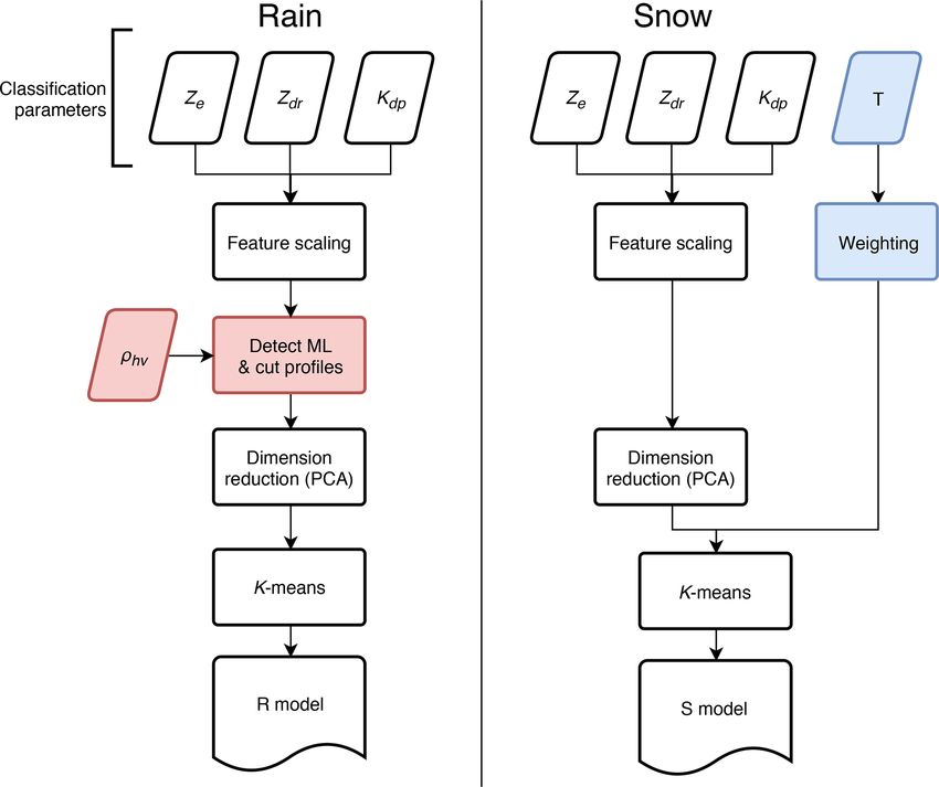
J. Tiira and D. Moisseev: Unsupervised classification of vertical profiles                                                          1231

Figure 1. Vertical profile clustering method for creating classification models for rain and snow events.

from the cluster mean. A value of a = 0.75 was used in this               explain the data well while being simple. Several methods
study.                                                                    exist for estimating the optimal number of classes. Neverthe-
                                                                          less, often domain- and problem-specific criteria have to be
3.2   Clustering                                                          applied for the best results.
                                                                             The optimal number of clusters depends on variability in
In the present study, the widely used k-means method was                  the data and correlations between different variables. The
chosen for clustering. The algorithm is known for its speed               more variability and degrees of freedom, the more clus-
and easy implementation and interpretation. Limitations of                ters are generally needed to describe different features in a
the method include the assumption of isotropic data space,                dataset. Since one important use case for the method is ice
sensitivity to outliers (Raykov et al., 2016) and the possibil-           process detection, particular attention is paid in separation of
ity to converge into a local minimum which may result in                  fingerprints of different processes between classes. An opti-
counterintuitive results. In our analysis, the anisotropy of the          mal set of classes would maximize this separation without in-
data space is partly mitigated by the PCA transformation. Af-             troducing too many classes to make their interpretation com-
ter the transformation, there is still anisotropy, but the transi-        plicated.
tions in density of the data points in PCA space are smooth                  As the problem of the number of classes is complex, it
(not shown), such that the k-means method seems to pro-                   is difficult to find an unambiguous quantitative measure for
duce clusters of meaningful sizes and shapes. The problem                 evaluating the correct number of classes. Attempts to create
of local minima is addressed using the k-means++ method                   a scoring function for optimizing the separation of ice pro-
(Arthur and Vassilvitskii, 2007) to distribute the initial clus-          cesses alone did not yield satisfactory results, but were rather
ter seeds in a way that optimizes their spread. The k-means++             used to support the manual selection process.
is repeated 40 times and the best result in terms of the sum of              Silhouette analysis (Rousseeuw, 1987), which is a method
squared distances of samples from their closest cluster center            for measuring how far each sample is from other clusters
is used for seeding.                                                      (separation) compared to its own cluster (cohesion), was
                                                                          also considered for selecting k. The metric, silhouette co-
3.3   Selecting the number of classes
                                                                          efficient s, takes values between −1 and 1. The higher the
An important consideration in using k-means clustering is                 value, the better the profile represents the cluster it is as-
the choice of number of clusters, k. A good model should                  signed to. A profile with s = 0 would be a borderline case be-

www.atmos-meas-tech.net/13/1227/2020/                                                        Atmos. Meas. Tech., 13, 1227–1241, 2020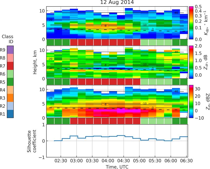
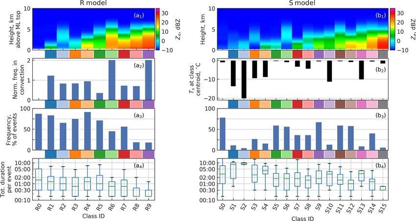
1232                                                J. Tiira and D. Moisseev: Unsupervised classification of vertical profiles

tween clusters, and negative values indicate that the profiles
mightP  have been assigned to wrong clusters. Silhouette score
s = k1 ki=1 si can generally be used for choosing k. Unfor-
tunately, when applied to the radar profile clustering results,
s decreases almost monotonically with increasing k in the
ranges of k analyzed and thus did not prove very useful for
this purpose. Rather, in this study, we calculate s for each
profile classification result individually as a measure of how
well the profile represents the class it is assigned to.
   The process of selecting the number of rain and snow pro-
file clusters, kR and kS , respectively, was as follows. First,
the k-means clustering was repeated 12 times for each k in
[5, 21] with 40 k-means++ initializations. This is where the
above-described silhouette analysis was performed for each
set of clusters and the stability of the initialization process
was analyzed for each k. Between the 12 repetitions, the clus-
tering converges to identical results for each kR < 12 and
kS < 10. With higher values of k, there are multiple solu-
tions to the clustering problem with only minor differences
between them. Moreover, the properties of the cluster cen-         Figure 2. Class centroid profiles of the R model. Profile counts per
troids are not highly sensitive to k. Clustering performed with    class are shown at the bottom omitting the count for low-reflectivity
k = k0 and k = k0 +1 would typically result in sets of clusters    class R0. Between the panes, each class has been assigned a color
sharing k0 − 1 to k0 very similar centroids.                       code.
   This stability of the clustering results makes it convenient
to select k manually. In the second stage, we analyzed each
separate clustering solution for differences between the clus-     Thus, a larger number of snow profile classes are needed to
ters from the point of view of snow processes and surface          meet the criteria described above. In clustering, there is a
precipitation. Specifically, an important criterion was to sep-    distinguishable separation between clusters representing Ts
arate the typical Kdp signatures of dendritic growth (e.g.,        close to 0 ◦ C and around −10 ◦ C. The vast majority of pro-
Kennedy and Rutledge, 2011) and the H–M process (Field             files belong to the warmer group.
et al., 2016) into different classes. On the other hand, the use      Taking all the mentioned considerations into account, we
of an unsupervised classification method should also allow         chose to use 10 and 16 classes for rain and snow profiles,
us to discover previously undocumented features in the radar       respectively. In 12 of the snow profile class centroids, Ts >
profiles if they are present in the data in significant numbers.   −5 ◦ C. In this paper, the rain and snow profile classification
   The goal in this step is to find as many significant unique     models are termed the R model and S model, respectively.
fingerprints with as low k as possible by manual evaluation.          In this section we have described our approach for opti-
Significant differences between clusters in this context in-       mizing the number of classes with the main criteria of sep-
clude variations in profile shapes and altitudes of charac-        arating the main profile characteristics and the fingerprints
teristics such as peaks, clear differences in echo-top heights     of ice processes into individual classes. It should be noted,
or differences of cluster centroid Ts of more than 3 ◦ C. The      however, that there is a large spectrum of research problems
most common trivial difference between a pair of clusters          and operational applications where an unsupervised profile
was a difference in the intensity of polarimetric radar vari-      classification method such as the one described in this paper
ables while the shapes of the cluster centroid profiles were       could be potentially useful. The optimal number of classes
almost identical. Altitude differences between fingerprints of     may depend on the application.
overhanging precipitation were also considered trivial.
   During this process, allowing some profile classes with
only trivial characteristics was inevitable in order to include    4   Results
others with significant unique fingerprints. For this reason,
some classes likely reflect natural variability of the same mi-    Class centroids of rain and snow profile classes are shown
crophysical process rather than unique processes and need to       in Figs. 2 and 3, respectively. The centroid profiles of dual-
be combined. However, the optimal way of combining the             polarization radar variables are inverse transformed from cor-
classes may depend on the application. Thus, we present the        responding centroids in PCA space. Classes are numbered in
classes uncombined in this paper.                                  the ascending order by the value of the first principal compo-
   In snow profile clustering, Ts as an extra classification       nent in the class centroids. By definition, the first component
parameter adds a significant additional degree of freedom.         has the largest variance and therefore has the biggest influ-

Atmos. Meas. Tech., 13, 1227–1241, 2020                                               www.atmos-meas-tech.net/13/1227/2020/
J. Tiira and D. Moisseev: Unsupervised classification of vertical profiles 1233
and 3, and comparing them to echo top heights in Fig. 4, it is
evident that Kdp layers, especially elevated ones, are strongly
associated with high echo tops.
The clustering results expose a prominent seasonal differ-
ence in Kdp intensity: consistently lower values are present in
snow events. There are four rain profile classes in contrast to
only two snow profile classes with peak cluster centroid Kdp
exceeding 0.1 ◦ km−1 . They represent total fractions of 13 %
and 4 % of rain and snow profiles, respectively. Correspond-
ing to this difference, in Figs. 2 and 3, as well as in Figs. 7
and 8 introduced later, Kdp is visualized in different ranges in
relation to rain and snow profiles. The seasonal differences in
ZDR and Ze intensities are less prominent. High Kdp in the
summer may be linked to higher water content during the
season. Additionally, the seasonal variability of vertical mo-
tion could impact the ZDR and Kdp enhancements.
Convection in the summer, especially in the presence of
hail, is linked to extreme values of radar variables and high
echo tops (Voormansik et al., 2017), which may also have a
small contribution to the seasonal differences (Mäkelä et al.,
2014). However, convective rainstorms are of short duration
and thus typically present in just a couple of profiles per con-
Figure 3. Class centroid profiles of the S model. The top panel vective cell. Therefore, their impact on the class properties is
shows class centroid surface temperatures. Profile counts per class expected to be limited. Manual analysis revealed that classes
are shown at the bottom omitting the count for low-reflectivity class R6 and R9 have the highest and R5 the lowest fractions of
S0. Between the panes, each class has been assigned a color code. profiles measured in convective cells. Further details of this
analysis are presented in Sect. 4.2.
Class frequencies are presented in the bottom panels of
ence on the clustering and classification results. The value of Figs. 2 and 3. Classes S0 and R0 represent very low values
this component is strongly correlated with intensities of Kdp of Ze throughout the column, i.e., profiles with very weak or
and Ze . no echoes. Therefore their frequencies depend merely on the
A number of class centroids in both classification models subjective selection of observation period boundaries and are
display distinct features in dual-polarization radar variables thus omitted in the figures. Boundaries of the precipitation
often linked to snow processes, such as peaks and gradients events are partly based on these two 0 classes. Events are
in Kdp and ZDR . Such features and their connection to other considered independent and separate if between them there
characteristics in the vertical structure of the profiles and fi- are profiles classified as S0 or R0 continuously for at least
nally to the precipitation processes are discussed in this sec- 12 h.
tion. With respect to Kdp intensity, classes in the R model can
As a general pattern in Figs. 2 and 3 we see that the high- be divided into four categories: R0 through R3 with negli-
est values of ZDR are associated with low echo tops while gible Kdp , low-Kdp classes R4 and R5 with max(Kdp,c ) ≈
the highest Kdp values occur in deeper clouds. This is in 0.04 ◦ km−1 , high-Kdp classes R6 and R7 with max(Kdp,c ) >
line with the previously reported findings (Kennedy and Rut- 0.11 ◦ km−1 , and classes R8 and R9 representing extreme
ledge, 2011; Bechini et al., 2013; Moisseev et al., 2015; values (max(Kdp,c ) ≈ 0.5 ◦ km−1 ). The subscript “c” denotes
Schrom et al., 2015; Griffin et al., 2018) that echo tops in the a class centroid value as opposed to values in individual pro-
DGL are associated with high ZDR and low Kdp in the layer, files. The peak Kdp,c of both R6 and R9 is at 3 km, cor-
whereas high Kdp in the DGL with low ZDR is associated responding to class mean GDAS temperatures of −16 and
with echo tops in T < −37 ◦ C where homogeneous freezing −18 ◦ C, respectively. Essentially, these two classes represent
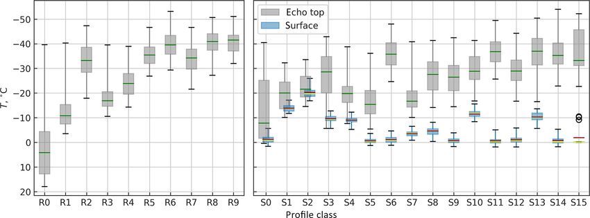
occurs. Using the NCEP GDAS model output, we analyzed clear Kdp features in the DGL.
the echo top temperatures, Ttop , of each vertical profile radar Classes R7 and R8 feature considerable Kdp in 2–3 km
observation. The results, grouped by profile class, are visu- thick layers right above the ML, with centroid values slightly
alized in Fig. 4. It should be noted that in the summer cold below 0.2 ◦ km−1 and around 0.4 ◦ km−1 , respectively. Es-
echo tops may be caused by strong updrafts in convection, sentially, both classes represent Kdp signatures in both the
whereas during the winter, echo tops colder than approxi- DGL and temperatures favored by the H–M process. Sinclair
mately −37 ◦ C are a more unambiguous indication of ho- et al. (2016) found that the typical Kdp values for the H–M
mogenous freezing. Inspecting the class centroids in Figs. 2 process are capped at 0.2. . .0.3 ◦ km−1 for the C band due to
www.atmos-meas-tech.net/13/1227/2020/ Atmos. Meas. Tech., 13, 1227–1241, 20201234 J. Tiira and D. Moisseev: Unsupervised classification of vertical profiles Figure 4. Cloud-top temperature distributions by class (gray) with the green line marking the medians. For S classes, surface temperature distribution is also shown (blue) with red lines marking the class centroid and yellow lines marking the median. Boxes extend between the first and the third quantiles, and whiskers cover 95 % of the data. Figure 5. The class S13 centroid is visualized in the three rightmost panes. Individual class member profiles are marked with thin lines. The pane on the left shows corresponding NCEP GDAS temperature profiles. The areas between the first and the third quantiles are shaded, radar data is in blue and GDAS is in gray. onset of aggregation. Based on this, it can be argued that R7 0.01 ◦ km−1 . These four low-reflectivity classes represent is a more likely indicator of H–M than R8. different surface temperatures, which is likely a major driver Classes R3 and R4 were found to often coexist in precipi- for the separation of these classes in the clustering process. tation events. Both are characterized by low Kdp and a layer Classes S4 and S5 represent low echo top profiles with high of ZDR in the DGL. In Fig. 4, we see that the echo tops are ZDR , with class centroid surface temperatures of −9.0 and lower for the R3 profiles, typically in the DGL. Therefore, −0.6 ◦ C, respectively. Further analysis of NCEP GDAS tem- we would expect growth of pristine crystals in low num- perature profiles reveals that, across the board, there is an in- ber concentrations and consequently with no significant ag- version layer present where radar profiles are classified as S4, gregation. This would explain why peak ZDR values from typically with temperatures below −10 ◦ C within the low- 3 to 5 dB are common in relation with R3. Profiles classi- est kilometer. This corresponds well with the bump in ZDR,c fied as R4, on the other hand, have slightly higher echo tops close to the surface, suggesting possible growth of pristine (T < −20 ◦ C), which are expected to result in higher num- dendrites within a strong inversion layer. In contrast, there is ber concentrations, leading to aggregation. The R4 profiles no inversion in connection with profiles belonging to S5, and are characterized by much lower ZDR values. the enhancement in ZDR occurs already at 2 to 3 km above In the S model (Fig. 3), classes S0 through S3 represent the surface, where the median NCEP GDAS temperature for profiles with low values of all three radar variables, each with S5 profiles is roughly between −18 and −10 ◦ C. S5 is the max(Ze,c ) < 0 dBZ, max(ZDR,c ) < 1 dB and max(Kdp,c ) < second most common class in S-model classification results. Atmos. Meas. Tech., 13, 1227–1241, 2020 www.atmos-meas-tech.net/13/1227/2020/
J. Tiira and D. Moisseev: Unsupervised classification of vertical profiles 1235
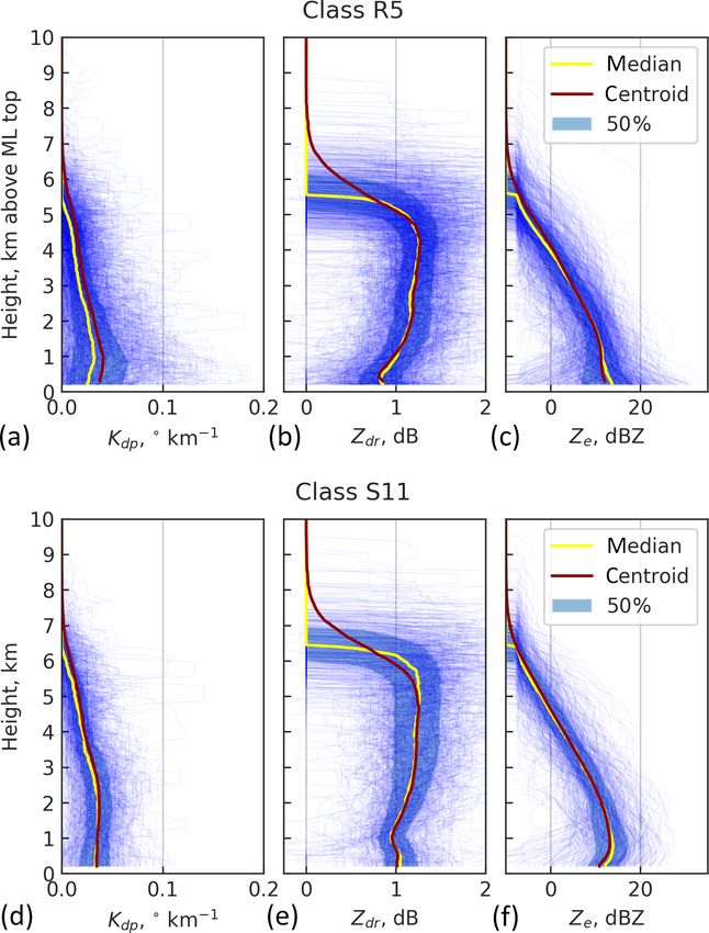
−6 ◦ C) are heavily contributed to by strong inversion layers.
The centroid and members of S13 are visualized in Fig. 5,
along with the member GDAS temperature profiles. The pro-
file class is characterized by a thick layer of considerable Kdp
from 2 to 3 km to the surface, and Ts ≈ −10 ◦ C. As seen in
the left panel of Fig. 5, S13 represents conditions where T
typically falls below −10 ◦ C close to the surface. This find-
ing suggests that a second DGL may occur in a strong inver-
sion layer.
Using the double-moment Morrison microphysics scheme
(Morrison et al., 2005), Sinclair et al. (2016) showed that
Kdp at the −8 to −3 ◦ C temperature range can be used for
identifying the H–M process. Such fingerprints are present in
particular in profiles classified as R7 or S12. However, man-
ual analysis of the profile data revealed that both of these
classes represent a mixture of fingerprints indicating H–M,
dendritic growth or the co-presence of both processes. In sev-
eral events, there were continuous time frames of profiles
classified as either R7 or S12 during which the altitude of
the Kdp signal was changing from profile to profile between
the DGL and 0 ◦ C level and was occasionally bimodal. One
example of such a time frame is shown in Fig. 7 and dis-
cussed further in Sect. 4.1.1. Some bimodality is also present
in the centroid Kdp,c of both classes, suggesting that the el-
evated Kdp,c values in the H–M region cannot be explained
solely by sedimenting planar crystals generated aloft but are
contributed by the H–M process.
Figure 6. Comparing classes R5 (a, b, c) and S11 (d, e, f) shows While there are no classes with clear-cut Kdp,c peaks at al-
evident similarities. Individual class member profiles are marked titudes corresponding to temperatures preferred by the H–M
with thin blue lines and the areas between the first and the third process in either rain or snow profile classification, there are,
quantiles are shaded with blue.
in contrast, several classes with strong elevated Kdp,c layers.
The proposal of Sinclair et al. (2016) that Kdp fingerprints of
the H–M process are not very pronounced may explain the
Classes S6 and S8 represent situations where precipitation tendency of the classification method not to produce more
is detached from the surface. These types of profiles are typi- pure H–M classes. Nevertheless, R7 and S12 can be used as
cally present in association with approaching frontal systems indicators for conditions where H–M may occur.
before the onset of surface precipitation. The most frequent Despite the differences in the classification methods for
class of the S model is S9 covering 13 % of the profiles. It rain and snow profiles, there are prominent similarities be-
represents moderate values of polarimetric radar variables tween the two models and profile classes therein. Archetypal
and cloud-top height. The most extreme values of reflectiv- classes such as high echo tops in the presence of elevated Kdp
ity and Kdp values in the S model are represented by classes layers (R6, R9, S14, S15) or high ZDR in shallow precipita-
S14 and S15. For both classes, Kdp,c peaks above 3 km, sug- tion (R3, S4, S5) exist in both classification models. Frequent
gesting dendritic growth in the member profiles. Values of classes R5 and S11, visualized side by side in Fig. 6, can
ZDR,c are significantly lower compared to other high echo be considered direct counterparts of each other. The vertical
top classes with weaker Kdp,c . Class S15 can be seen as a structure of polarimetric radar variables above the ML in R5
more extreme variant of S14 with much stronger Kdp,c and match strikingly well with S11. The two classes are charac-
Ze,c . In addition, S15 represents lower values of ZDR near terized by weak Kdp and typical values of ZDR slightly above
the DGL, having slightly elevated values in the bottom 3 km 1 dB aloft, decreasing towards the altitude corresponding to
instead. These differences are likely due to even higher ice 0 ◦ C. Presumably, this indicates the presence of aggregation.
number concentrations in S15 profiles, which lead to more
intense aggregation. 4.1 Case studies
Comparing class centroid Ts and class frequencies in Fig. 3
it can be seen that most snowfall occurs at Ts ≈ 0 ◦ C. Fur- In Figs. 2 and 3, each class is assigned a color code (between
ther analysis of GDAS temperature profiles for the snow the panels). This color coding is used in Figs. 7 and 8 to mark
events revealed that typically cold surface temperatures (Ts < classification results in a rain and a snow case, respectively.
www.atmos-meas-tech.net/13/1227/2020/ Atmos. Meas. Tech., 13, 1227–1241, 20201236 J. Tiira and D. Moisseev: Unsupervised classification of vertical profiles
Figure 7. Classification analysis of a rain case with silhouette
scores. The automatically detected melting layer is marked with a
dashed line, the solid lines show the NCEP GDAS temperature con-
tours and the colors between the panes denote classification results. Figure 8. Classification analysis of a snow case with silhouette
scores. Solid lines show the NCEP GDAS temperature contours and
the colors between the panes denote classification results.
Note that the same set of colors is used for denoting rain and
snow profile classification, but they should not be confused with varying altitude. Without in situ observations or analysis
with each other. of Doppler spectra, it is not trivial to tell whether this vari-
ability is due to co-presence of dendritic growth and H–M or
4.1.1 12 August 2014 simply fall streaks. Class R6, on the other hand, is more spe-
cific to a Kdp fingerprint in the DGL. The more infrequent
In Fig. 7, rain profile classification has been applied to a profiles with clear Kdp bands above the DGL are typically
precipitation event from 12 August 2014. During this event, also classified as R6 or R9.
echo tops repeatedly exceed 10 km. Only the parts of the pro-
files above the melting layer top are analyzed here, since ev- 4.1.2 15–16 February 2014
erything below that level is invisible to the classifier. The first
two and the last two profiles shown in the figure are charac- Classification results for 15–16 February 2014 are shown
terized by low Ze and low Kdp , while ZDR has values around in Fig. 8. The event has a clear structure of an approach-
1 dB. These profiles are classified as R5 (dark green). Be- ing frontal system. Between 17:00 and 18:00 UTC Ze is very
tween 02:30 and 03:00 UTC, a significant increase in Kdp low, corresponding to class S0, which is marked with white
occurs, followed by an increase in reflectivity and decrease color between the panels. Between 18:00 and 21:00 UTC,
in ZDR . The temperature (altitude) of the downward increase the event starts with overhanging precipitation, classified as
in Kdp varies from the −20 ◦ C level to closer to the ML. In S6 (light green). This is followed by light precipitation with
this phase, there is also a small increase in ZDR in the DGL echo tops at roughly 7 to 8 km and relatively high ZDR near
whenever the increase in Kdp also occurs in the DGL. This the echo top, decreasing downwards. This corresponds well
phase in the event is sustained until around 05:00 UTC and with class S11 (dark brown). After 23:30 UTC, The echo top
is classified as R7 (dark red). It is followed by approximately height is decreased to roughly 6 km, ZDR is decreased and
an hour of a weaker elevated Kdp layer at around 4 to 6 km Kdp signals appear close to ground level. The increase in Kdp
altitude with profiles classified as class R6 (light green). The occurs within the −8 to −3 ◦ C temperature range, suggest-
silhouette coefficient is positive throughout the event indicat- ing the presence of the H–M process. Indeed, Kneifel et al.
ing good confidence of the classification results. The silhou- (2015) report needles, needle aggregates and rimed particles
ette of the profiles classified as R6 is not very high, though, on the surface at the measurement site during this period and
which is likely due to lower values of Ze compared to the favorable conditions for rime splintering. Further, using the
class centroid. Weather Research and Forecast (WRF) model, Sinclair et al.
Similar analysis of more rain events in the dataset reveals (2016) showed that secondary ice processes are needed to
that, similar to the 12 August event, R7 typically coincides explain the observed number concentrations during this time
with an increase in Kdp in the DGL, H–M layer or both, often period. The corresponding profiles are classified as S12 (light
Atmos. Meas. Tech., 13, 1227–1241, 2020 www.atmos-meas-tech.net/13/1227/2020/J. Tiira and D. Moisseev: Unsupervised classification of vertical profiles 1237
brown). Within this case study, two profiles, marked with of Kdp , ZDR and Ze and surface temperature. It was applied
dark purple, are classified as S9, likely due to the momen- to vertical profile data extracted from C-band RHI scans over
tary absence of any strong Kdp or ZDR signals. Hyytiälä measurement station in southern Finland. We ap-
plied separate versions of the method based on if surface
4.2 Statistics precipitation type was rain (R model) or snow (S model).
In the R model, profiles are truncated at the melting layer
Frequency statistics of the profile classes are presented in top, and in the S model surface temperature is used as an
Fig. 9. We analyzed a subset of rain events as either con- additional classification feature. The content of the vertical
vective or stratiform using a number of sources of publicly profile classes was manually interpreted.
available satellite and numerical model data. Out of 70 events In the present investigation, some class centroids resem-
analyzed, 15 were convective and 55 stratiform. Panel (a2 ) in bled textbook examples of previously documented snow pro-
Fig. 9 shows the ratios of the number of profiles in convec- cess fingerprints, while others may represent a mixture of dif-
tive cases per class to the expected value in uniform distri- ferent conditions. If temperature profiles from either sound-
bution. On average, twice as many profiles are classified as ings or numerical models are available, the interpretation can
R6 and R9 in convective situations compared to their aver- be done in the absence of surface crystal type reports. No-
age frequencies. Both classes are characterized by high echo tably, this is prerequisite in cases of rainfall when direct ob-
tops and elevated Kdp bands. On the other hand, classes servations of crystal types cannot be performed at the sur-
R7 and R8, also representing high Kdp values, but closer face.
to the melting layer than R6 and R9, appear in lower-than- The year-round variability in the vertical structure of Kdp ,
average frequency in convective situations. Class R5 is most ZDR and Ze can be described using a total of 26 profile
pronouncedly characteristic for stratiform events, with fre- classes: 10 and 16 in the presence and absence of the ML,
quency in convective events roughly one-third of the average respectively. One of the main goals of this study was to
value. associate profile classes with snow processes for their au-
Panels (a3 ) and (b3 ) of Fig. 9 show the fractions of in- tomated identification. It should be noted, though, that the
dependent precipitation events in which each class occurs. profile classification is not based on expressly selected char-
With rain events, this frequency correlates inversely with acteristics of radar fingerprints of the processes, but rather
Kdp,c . Rain profiles classified as R8 and R9, which repre- the general, complete structure of the profiles. Nevertheless,
sent the strongest Kdp signatures, occur in 20 % and 19 % of some profile classes seem to be strong indicators of specific
the events, respectively, with at least one of the two occurring processes or their combinations within the vertical profiles.
in 25 % of the events. Classes R6 and R7, representing more From both classification models we can identify a total of
modest Kdp features, occur in 45 % and 57 % of cases, re- seven archetypes with the following characteristics.
spectively, and the rest of the classes between 67 % and 92 %
of the cases. 1. Profiles have a strong Kdp peak in the DGL, while the
With snow events, the likelihood of a given class occur- peak in ZDR is not pronounced. This archetype appears
ring within an event correlates not only with peak Kdp,c but in deep precipitation systems with homogeneous freez-
also with surface temperature. Any class representing low ing at the cloud top. It is associated with intensified den-
Kdp values and surface temperature close to 0 ◦ C occurs in dritic growth leading to aggregation and high precipita-
more than half of the snow events. tion rate. (Classes R6, R9, S14, S15)
The per precipitation event class persistence is visualized 2. There is a Kdp signature between the DGL and the 0 ◦ C
in the bottom panels of Fig. 9. Profile classes representing level, possibly due to simultaneous occurrence of den-
the highest values of Ze at the surface, namely R6–R9, S12, dritic growth and secondary ice production. Homoge-
S14 and S15, are short-lived, whereas snow profile classes neous freezing occurs at the cloud top. (R7, R8, S12)
characterized by cold surface temperatures are the most per-
sistent. Profiles classified as R0 or S0 omitted, the median 3. Profiles are characterized by high echo tops, negligi-
durations of rain and snow events in the dataset are 5.5 and ble Kdp , and ZDR > 1 dB, which decreases closer to
11.5 h, respectively. This difference explains why S classes the melting level due to aggregation. Typically, Ze <
are on average more persistent than R classes. 20 dBZ. (R5, S11)
4. The cloud top is between the −30 and −20 ◦ C levels,
and there is only a weak ZDR band present at the −15 ◦ C
5 Conclusions level. Ze is moderate at roughly 20–30 dBZ, and Kdp is
weak. (R4, S9)
A novel method of dual-polarization radar profile classifi-
cation for investigating vertical structure of snow processes 5. ZDR is typically higher than 1.5 dB at the cloud to at
in the profiles was presented in this paper. The method is around −15 ◦ C and is associated with the growth of
based on clustering of PCA components of vertical profiles pristine planar crystals in low number concentrations.
www.atmos-meas-tech.net/13/1227/2020/ Atmos. Meas. Tech., 13, 1227–1241, 20201238 J. Tiira and D. Moisseev: Unsupervised classification of vertical profiles
Figure 9. Statistics on frequency of each profile class. Classes are identified by class centroid Ze (a1, b1) and class centroid Ts for snow
profile classes (b2), with color codes between the panels and class IDs at the bottom. Panel (a2) has the ratios of the number of profiles
in convective cases per class to the expected value in uniform distribution. In (a4, b4), the class frequencies are given as percentage of
events (a3, b3) and total durations (a4, b4) within events.
No Kdp is present, and low values of Ze indicate the However, there are possible drawbacks in the data-driven
absence of aggregation. (R3, S5) approach. The typical radar fingerprints of the H–M process
were found to be much more scarce than those of dendritic
6. The radar echo is detached from the surface either due growth, and often less pronounced. This negatively affects
to snow particles not having reached the surface yet or how the typical fingerprints of the H–M process are repre-
because they are sublimating due to a dry layer. (R2, S3, sented in the classes. This could be enhanced by introducing
S6, S8) a larger fraction of H–M profiles in the training data.
Another disadvantage in the data-driven approach is that
7. Ze is weak throughout the profile. (R0, S0–S2) covering a meaningful collection of unique fingerprints re-
quires a large number of clusters, some of which do not rep-
In addition to these archetypes found in both summer and resent unique microphysical processes. This problem may be
winter storms, there are S classes representing situations mitigated to some extent by further optimizing the scaling
where strong inversions interfere with snow processes. No- of the radar variables such that the clustering would be less
tably, we found indications of dendritic growth in strong in- driven by differences in the intensities of the signatures in
version layers, manifested as class S13. As the colder arctic contrast to their shapes. Another way to address this issue is
air mass seldom occurs in southern Finland, Ts < −10 ◦ C can to simply combine classes that seem to represent the same
usually be attributed to a strong lower-level inversion. Such processes, in like manner of the archetypes presented above.
inversions may have an important effect on the frequency Reducing the number of classes by simply choosing a smaller
of occurrence of some ice processes. Further, this implies k in the k-means clustering would reduce the amount of man-
that temperature information near the surface is necessary in ual work involved in defining the class boundaries at the cost
order to determine whether a low altitude Kdp signature in of decreased detail and accuracy in separating the processes.
the winter is an implication of the H–M process or dendritic With a smaller k, the clustering would be driven by more
growth. general features of the profiles such as the overall shape and
Our approach to the classification problem is pro- intensity of the polarimetric radar variables, whereas espe-
nouncedly data-driven. This way, if the training material rep- cially the typical characteristics of the H–M process finger-
resents the climatology of ice processes and their radar sig- prints involve a higher level of detail.
natures, as was the aim in this study, the resulting classes The classification method presented in this study should
will reflect the statistical properties of this climatology. Hand be considered a starting point in studying vertical profiles
picking the training material, on the other hand, would intro- of radar variables using unsupervised classification. As such,
duce human bias into the class boundaries.
Atmos. Meas. Tech., 13, 1227–1241, 2020 www.atmos-meas-tech.net/13/1227/2020/J. Tiira and D. Moisseev: Unsupervised classification of vertical profiles 1239
there is a vast range of potentially useful opportunities for investigating the use of unsupervised profile classification in
further development of the method. The method is built on such applications.
reasoned use of well-known, proven algorithms such as PCA
and k-means. We showed that this combination of machine
learning algorithms allows both identification of known fin- Data availability. The FMI radar and surface temperature data are
gerprints and a more explorative approach in studying the available from the Finnish Meteorological Institute (2019) open
characteristics of a regional climatology of precipitation pro- data portal: https://en.ilmatieteenlaitos.fi/open-data-sets-available
cesses. Limitations of the k-means method include the spher- (last access: 1 October 2019).
ical shape and similar area occupied by the clusters, which
involve a risk of suboptimal separation of the microphysi-
Supplement. The supplement related to this article is available on-
cal processes to different classes. In this study, we addressed
line at: https://doi.org/10.5194/amt-13-1227-2020-supplement.
these limitations by allowing a rather large number of ini-
tial classes and combining similar ones by identifying the
archetypes based on known fingerprints of the processes. An-
Author contributions. The study was designed by both authors. JT
other possible approach would be to explore the numerous implemented and ran the classification and made the figures. JT
alternative clustering methods for a more optimal separation wrote the manuscript, with contributions from DM. Both authors
of the precipitation processes. A comprehensive comparison discussed the results and commented on the manuscript.
of such methods, however, is outside the scope of this study.
In the present classification method, ambient temperature
is known only at the profile base. Compared to the use of Competing interests. The authors declare that they have no conflict
full temperature profiles, this simplifies the method and, per- of interest.
haps even more importantly, the requirements for the input
data. However, future studies should investigate if the use of
full temperature profiles allows more accurate separation of Acknowledgements. We would like to thank the personnel of
precipitation processes into different classes. Hyytiälä station and Matti Leskinen for their support in field ob-
The unsupervised nature of the classification method is ex- servation.
pected to allow extension of its application to the detection
of ice processes not covered in this study. Recently, Li et al.
(2018) showed that certain combinations of Ze , ZDR and Kdp Financial support. This research has been supported by the
Academy of Finland’s Center of Excellence (CoE) (grant no.
signatures can potentially be used for detecting heavy riming.
307331). The research of Jussi Tiira has been supported by
Furthermore, the process is frequently observed in Finland, the Doctoral Programme in Atmospheric Sciences (ATM-DP,
highlighting the potential of using an unsupervised method University of Helsinki).
for its identification.
It should be noted that wind shear effects induce differen- Open access funding provided by Helsinki University Library.
tial advection of hydrometeors at different altitudes, affect-
ing the gradients in the vertical profiles of radar variables
(Lauri et al., 2012). Therefore caution should be used in inter- Review statement. This paper was edited by S. Joseph Munchak
preting microphysical processes corresponding to class cen- and reviewed by two anonymous referees.
troid profiles. The wind shear effects are difficult to correct
for using vertical profile or RHI radar observations due to
the limitations in horizontal sampling. Such adjustments be- References
come more viable if classification is performed on profiles
extracted from volume scans, which will be investigated in Andrić, J., Kumjian, M. R., Zrnić, D. S., Straka, J. M., and Mel-
future work. nikov, V. M.: Polarimetric Signatures above the Melting Layer in
The ability to describe a climatology of vertical structure Winter Storms: An Observational and Modeling Study, J. Appl.
of dual-polarization radar variables and, further, precipita- Meteorol. Clim., 52, 682–700, https://doi.org/10.1175/JAMC-D-
tion processes using a finite number of classes has evident 12-028.1, 2013.
potential in improving quantitative precipitation estimation. Arthur, D. and Vassilvitskii, S.: k-means++: The advantages of
careful seeding, 1027–1035, Society for Industrial and Applied
We anticipate that automated detection of ice processes may
Mathematics, 2007.
allow the development of adaptive relation for snowfall rate Bechini, R. and Chandrasekar, V.: A Semisupervised Ro-
S = S(Ze ), in which the parameters could be chosen based bust Hydrometeor Classification Method for Dual-Polarization
on the profile classification result. Adaptive S(Ze ) relations, Radar Applications, J. Atmos. Ocean. Tech., 32, 22–47,
in turn, have potential in improving the vertical profile of re- https://doi.org/10.1175/JTECH-D-14-00097.1, 2015.
flectivity correction methods. Future work will be devoted to Bechini, R., Baldini, L., and Chandrasekar, V.: Polarimetric Radar
Observations in the Ice Region of Precipitating Clouds at C-Band
www.atmos-meas-tech.net/13/1227/2020/ Atmos. Meas. Tech., 13, 1227–1241, 2020You can also read