Intercomparison of lidar, aircraft, and surface ozone measurements in the San Joaquin Valley during the California Baseline Ozone Transport Study ...
←
→
Page content transcription
If your browser does not render page correctly, please read the page content below
Atmos. Meas. Tech., 12, 1889–1904, 2019
https://doi.org/10.5194/amt-12-1889-2019
© Author(s) 2019. This work is distributed under
the Creative Commons Attribution 4.0 License.

Intercomparison of lidar, aircraft, and surface ozone measurements
in the San Joaquin Valley during the California Baseline Ozone
Transport Study (CABOTS)
Andrew O. Langford1 , Raul J. Alvarez II1 , Guillaume Kirgis1,2 , Christoph J. Senff1,2 , Dani Caputi3 ,
Stephen A. Conley4 , Ian C. Faloona3 , Laura T. Iraci5 , Josette E. Marrero5,a , Mimi E. McNamara5,7,b , Ju-Mee Ryoo5,c ,
and Emma L. Yates5,6
1 Chemical   Sciences Division, NOAA Earth System Research Laboratory, Boulder, CO 80305, USA
2 Cooperative  Institute for Research in Environmental Sciences, University of Colorado, Boulder, CO 80309, USA
3 Department of Land, Air, and Water Resources, University of California, Davis, CA 95616, USA
4 Scientific Aviation, Inc., Boulder, CO 80301, USA
5 Atmospheric Science Branch, NASA Ames Research Center, Moffett Field, CA 94035, USA
6 Bay Area Environmental Research Institute, Petaluma, CA 94952, USA
7 Environmental Science and Policy Department, University of California, Davis, CA 95616, USA
a now at: Sonoma Technology, Inc., Petaluma, CA 94954, USA
b now at: Illingworth & Rodkin, Inc., Petaluma, CA 94954, USA
c now at: Science and Technology Corporation, Moffett Field, CA 94035, USA

Correspondence: Andrew O. Langford (andrew.o.langford@noaa.gov)

Received: 27 September 2018 – Discussion started: 23 October 2018
Revised: 16 February 2019 – Accepted: 6 March 2019 – Published: 25 March 2019

Abstract. The California Baseline Ozone Transport Study           measurements agree, on average to within 5 ppbv, the sum of
(CABOTS) was conducted in the late spring and summer of           their stated uncertainties of 3 and 2 ppbv, respectively.
2016 to investigate the influence of long-range transport and
stratospheric intrusions on surface ozone (O3 ) concentrations
in California with emphasis on the San Joaquin Valley (SJV),
one of two extreme ozone non-attainment areas in the US.          1   Introduction
One of the major objectives of CABOTS was to character-
ize the vertical distribution of O3 and aerosols above the SJV    The San Joaquin Valley (SJV) of California is one of only
to aid in the identification of elevated transport layers and     two “extreme” ozone (O3 ) non-attainment areas remaining
assess their surface impacts. To this end, the NOAA Earth         in the United States with a 2016 ozone design value, i.e.,
System Research Laboratory (ESRL) deployed the Tunable            the metric used by the U.S. EPA to determine air quality
Optical Profiler for Aerosol and oZone (TOPAZ) mobile lidar       compliance that is calculated as the 3-year average of the
to the Visalia Municipal Airport (36.315◦ N, 119.392◦ E) in       fourth highest measured maximum daily 8 h average mix-
the central SJV between 27 May and 7 August 2016. Here we         ing ratio (MDA8), which is more than 20 parts per bil-
compare the TOPAZ ozone retrievals with co-located in situ        lion by volume (ppbv) greater than the primary National
surface measurements and nearby regulatory monitors and           Ambient Air Quality Standard (NAAQS) of 70 ppbv (https:
also with airborne in situ measurements from the University       //www3.epa.gov/airquality/greenbook/hdtc.html, last access:
of California at Davis–Scientific Aviation (SciAv) Mooney         18 March 2019). Such high O3 concentrations are harm-
and NASA Alpha Jet Atmospheric eXperiment (AJAX) re-              ful to human health (U.S. Environmental Protection Agency,
search aircraft. Our analysis shows that the lidar and aircraft   2014) and impair plant growth and productivity (Avnery et
                                                                  al., 2011a, b), adversely affecting both the USD 15 billion

Published by Copernicus Publications on behalf of the European Geosciences Union.
1890                           A. O. Langford et al.: Intercomparison of lidar, aircraft, and surface ozone measurements

annual crop yield (https://quickstats.nass.usda.gov/results/      2     California Baseline Ozone Transport Study
9438C760-67AB-3AFB-B182-8484DB20A903, last access:                      (CABOTS)
18 March 2019) in the SJV and the iconic forests of the
nearby Sequoia National Park and Kings Canyon National            The CABOTS field campaign was conducted between mid-
Park (Panek et al., 2013).                                        May and mid-August of 2016. The primary measurements
   The need to better understand the causes for the high          (see Fig. 1a) included electrochemical cell (ECC) ozoneson-
surface O3 in the San Joaquin Valley has motivated sev-           des (Johnson et al., 2002) launched daily from Bodega
eral major air quality studies over the years including the       Bay (38.319◦ N, 123.075◦ E, 12 m above mean sea level,
San Joaquin Valley Air Quality Study (SJVAQS) in 1990             a.s.l.) (6 May–17 August) and Half Moon Bay (37.505◦ N,
(Lagarias and Sylte, 1991), the Central California Ozone          122.483◦ E, 9 m a.s.l.) (15 July–17 August) by the San Jose
Study (CCOS) in 2000, (Reynolds et al., 2010) and the Cal-        State University (SJSU), in situ aircraft sampling of O3 and
ifornia Research at the Nexus of Air Quality and Climate          other compounds above central California by the University
Change (CalNex) field campaign in 2010 (Ryerson et al.,           of California, Davis (UC Davis)–Scientific Aviation (Trous-
2013; Brune et al., 2016). More recently, this issue was          dell et al., 2016) and the NASA Alpha Jet Atmospheric
addressed by the 2016 California Baseline Ozone Trans-            eXperiment (AJAX) (Yates et al., 2015), and ozone and
port Study (CABOTS) organized and supported by the Cal-           backscatter lidar measurements by the truck-based NOAA
ifornia Air Resources Board (CARB) (https://www.arb.ca.           ESRL TOPAZ lidar system (Alvarez et al., 2011) at the
gov/research/cabots/cabots.htm, last access: 18 March 2019).      Visalia Municipal Airport (VMA, 36.315◦ N, 119.392◦ E,
CABOTS was designed to investigate the contributions of           88 m a.s.l.) (27 May–18 June and 18 July–7 August) (Fig. 2).
background O3 (Jaffe et al., 2018) and the influence of strato-   Surface O3 measurements were also made at the ozonesonde
spheric intrusions (Lin et al., 2012a) and long-range trans-      and lidar sites and at the UC Davis monitoring station
port from Asia (Lin et al., 2012b) on surface O3 concen-          at the Chews Ridge Observatory (36.306◦ N, 121.567◦ E,
trations in the SJV during late spring and summer. Char-          1520 m a.s.l.) (Asher et al., 2018) in the Santa Lucia Moun-
acterization of the vertical distribution of O3 in the lower      tains west of Visalia, as well as using the extensive networks
and middle free troposphere above the SJV and upwind re-          of regulatory surface monitors maintained by the California
gions with an accuracy of at least 10 %, the nominal accuracy     Air Resources Board and the San Joaquin Valley Air Pollu-
of ECC ozonesondes in the troposphere (Smit et al., 2014),        tion Control District (SJVAPCD).
was a key objective of the campaign, and O3 profiles were            The Bodega Bay and Half Moon Bay sites were located
measured using three different techniques (lidar, aircraft, and   on the coast to sample the Pacific inflow, and the VMA was
ozonesondes) in various parts of California. Integration of       chosen for the TOPAZ operations because of its central loca-
these datasets requires that these measurements be intercom-      tion in the SJV, the availability of the runway and airspace
pared (Ancellet and Ravetta, 2005; Beekmann et al., 1995;         for low approaches and aircraft profiles, and the presence
Kempfer et al., 1994; Schäfer et al., 2002) and any differ-       of the co-located SJVAPCD wind profiler and radio acous-
ences among the various techniques understood and charac-         tic sounding system (RASS) (Bao et al., 2008). The TOPAZ
terized. For pollution studies it is important that this vali-    truck was parked on the west side of the VMA between the
dation includes the lowest 100 m, which is inaccessible to        airport runway and the heavily trafficked multilane CA-99
most ozone lidars (Wang et al., 2017). In this paper, we com-     and adjacent San Joaquin Valley Railroad (SJVR) (Fig. 2).
pare O3 measurements from the NOAA Earth System Re-               The VMA is located about 10 km west of downtown Visalia
search Laboratory ESRL multi-angle Tunable Optical Pro-           (pop. 130 000) and lies about one-third (60 km) of the way
filer for Aerosol and oZone (TOPAZ) lidar with in situ mea-       from Fresno to Bakersfield (Fig. 1a, b). Visalia is located
surements from nearby regulatory and research surface mon-        about 400 km from Bodega Bay and 300 km from Half Moon
itors, and also with instruments flown aboard the UC Davis–       Bay, which limited the usefulness of comparisons between
Scientific Aviation Mooney (Trousdell et al., 2016) and Al-       the lidar and ozonesondes.
pha Jet research aircraft based at NASA’s Ames Research
Center (Hamill et al., 2016; Yates et al., 2015). These com-
parisons, together with those from the multi-lidar (including     3     Ozone measurement platforms
TOPAZ) and ozonesonde Southern California Ozone Obser-
vation Project (SCOOP) intercomparison conducted by the           3.1    NOAA-ESRL TOPAZ lidar
NASA-sponsored Tropospheric Ozone Lidar Network (TOL-
Net) immediately after CABOTS (Leblanc et al., 2018), pro-        The TOPAZ differential absorption lidar (DIAL) system was
vide this validation.                                             originally developed for the profiling of O3 and particulate
                                                                  backscatter in the planetary boundary layer and lower free
                                                                  troposphere from NOAA Twin Otter aircraft (Alvarez et al.,
                                                                  2011; Langford et al., 2010, 2011, 2012; Senff et al., 2010).
                                                                  The lidar was reconfigured for mobile ground-based mea-

Atmos. Meas. Tech., 12, 1889–1904, 2019                                             www.atmos-meas-tech.net/12/1889/2019/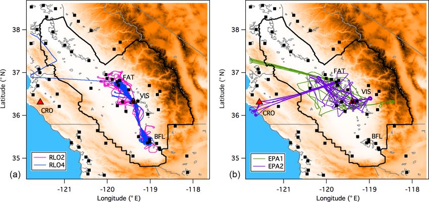
A. O. Langford et al.: Intercomparison of lidar, aircraft, and surface ozone measurements 1891
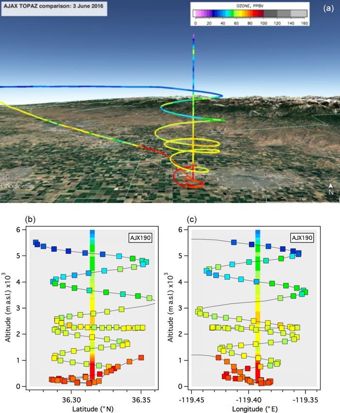
Figure 1. (a) Topographic map showing the air basins of California (dashed black lines); the San Joaquin Valley Air Basin (SJVAB) is
outlined in heavy solid black. Interstate highways and urban areas are shown in gray. The filled red triangles show the CABOTS measurement
sites at Bodega Bay (BBY), Half Moon Bay (HMB), Visalia Municipal Airport (VMA), and Chews Ridge Observatory (CRO). (b) The same
as (a) but showing an enlarged view of the area surrounding the VMA. The solid and dotted–dashed gray lines represent the major highways
and railroads, respectively, with the heavier solid line showing CA-99 (see text). The filled black squares show the six closest regulatory O3
monitors active during the CABOTS campaign: Visalia (VIS), Hanford (HFD), Santa Rosa Rancheria (SRR), Fresno–Drummond St. (FRD),
Parlier (PRL), and Porterville (PRV). The elevation scale is the same as in (a).
for in situ O3 measurements (2B Technologies model 205)
that samples air 5 m above the surface and an Airmar 150WX
weather station to measure temperature, pressure, relative hu-
midity, and wind speed and direction. The 2B model 205 has
been approved by the EPA as a federal equivalent method
(FEM) for surface O3 monitoring and has a nominal (1σ )
precision and accuracy that is the greater of 1 ppbv or 2 % for
10 s averages. Modified versions of the same instrument were
flown on both the Scientific Aviation Mooney and NASA Al-
pha Jet. Comparisons between the NOAA 2B at the VMA
and a mobile calibration source operated by CARB revealed
a 3 % low bias in the recorded 2B measurements that has
been corrected in the data used here.
The eye-safe TOPAZ lidar is built around a low pulse
energy (∼ 100 µJ), high repetition rate (1 kHz) quadrupled
Nd:YLF pumped Ce:LiCAF laser that is retuned between
Figure 2. Aerial view of the Visalia Municipal Airport (VMA) each pulse to generate light at three different wavelengths
showing the 1 km lidar slant path line of sight as a yellow arrow from 286 to 294 nm with an effective repetition rate of
with the TOPAZ truck located at the base. The Scientific Avia- 333 Hz for each wavelength (Alvarez et al., 2011). The laser
tion Mooney and AJAX Alpha Jet are shown flanking the NOAA pulses are transmitted and the lidar return signals collected
ESRL TOPAZ truck below the Google Earth image. Mooney and by a coaxial transmitter and receiver equipped with a com-
TOPAZ photos by Andrew O. Langford. Alpha Jet photo by Wil- mercial (Licel) photomultiplier-based dual analog or photon
fred von Dauster. counting system. This hybrid data acquisition system was in-
stalled in 2016 and replaced the original fast analog data ac-
quisition system that was optimized for aircraft operations
surements in 2012 and deployed in this configuration to sev-
(Alvarez et al., 2011; Wang et al., 2017). This modification
eral field campaigns including the 2013 Las Vegas Ozone
increased the maximum useful range to ∼ 6 km during the
Study (LVOS) (Langford et al., 2015) prior to CABOTS.
day and to more than 8 km at night, depending on the laser
The lidar is installed in the back of a medium box truck (see
power, atmospheric extinction, and solar background light.
Fig. 2) equipped with a commercial UV absorption monitor
www.atmos-meas-tech.net/12/1889/2019/ Atmos. Meas. Tech., 12, 1889–1904, 2019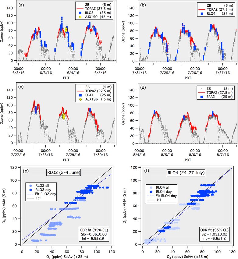
1892                            A. O. Langford et al.: Intercomparison of lidar, aircraft, and surface ozone measurements

   The truck-mounted version of TOPAZ incorporates a large          lidar location were used to account for the temperature de-
scannable turning mirror above the vertically pointing trans-       pendence of the O3 cross sections and to convert O3 number
mitter and receiver to allow profile measurements at differ-        densities to mixing ratios. The total uncertainties in the 8 min
ent slant angles. These slant profiles can be combined to           ozone retrievals in the absence of strong aerosol gradients are
create vertical profiles that start much closer to the ground       estimated to increase from ±3 ppbv below 4 km to ±10 ppbv
(25–30 m) than conventional vertically staring lidar systems        at the top of the profile. When strong backscatter gradients
(Proffitt and Langford, 1997). During CABOTS, the scan-             are present, the O3 uncertainty can potentially increase by
ning mirror was moved sequentially between elevation an-            another ±3 ppbv.
gles of 90, 20, 6, and 2◦ with a 225 s averaging time at 90◦
and 75 s averaging times at the other three angles. The cycle       3.2   UC Davis–Scientific Aviation Mooney
was repeated approximately every 8 min and the vertical pro-
jections combined to create a single vertical profile starting at   The University of California at Davis and Scientific Avi-
27.5±5 m above ground level (a.g.l.). This approach assumes         ation, Inc. (http://www.scientificaviation.com, last access:
a fair degree of horizontal homogeneity and the lidar slant         18 March 2019) conducted a series of research flights
paths were oriented parallel to the VMA runway (135◦ ) over         above the SJV during the summer of 2016 using a Sci-
open farmland to avoid populated neighborhoods and mini-            entific Aviation single-engine Mooney TLS or Ovation
mize the effects of NO emissions from the often heavy traffic       aircraft as part of the CARB-supported Residual Layer
on CA-99 (see Fig. 2), which could locally titrate ozone and        Ozone Study (RLO) (https://www.arb.ca.gov/research/apr/
create strong horizontal concentration gradients near the sur-      past/14-308.pdf, last access: 18 March 2019). Several of
face.                                                               these flights overlapped with the TOPAZ operations during
   The O3 profiles shown here were retrieved using two              CABOTS, as did some of the 12 additional flights (EPA)
wavelengths (∼ 287 and 294 nm) with 30 m range gates and a          funded by the U.S. EPA and the Bay Area Air Quality Man-
smoothing filter that increased from 270 m wide at the min-         agement District (BAAQMD). The Mooney carried a 2B
imum range (815 ± 15 m) to 1400 m wide at the maximum               Technologies model 205 O3 monitor, an EcoPhysics model
range (8 km). The effective vertical resolution increased from      CLD88 (NO) with a photolytic converter to measure NO
∼ 10 m near the surface to ∼ 150 m above 500 m a.g.l. and           and NO2 , and a Picarro 2301f cavity ring-down spectrom-
900 m at 6 km. Profiles of the backscatter from aerosols,           eter (CRDS) to measure CO2 , CH4 , and H2 O (Trousdell et
smoke, and dust were retrieved with a constant 7.5 m reso-          al., 2016). The 2B model 205 was used with the minimum
lution at 294 nm. The ozone profiles were computed using            integration time of 2 s, which corresponds to a mean distance
the O3 absorption cross sections from Malicet et al. (1995)         of 150 m at the typical level flight speed (the data stream
and an iterative technique to correct for differential aerosol      was sampled at 1 s intervals). As noted above, the 2B has
backscatter and extinction that assumes a backscatter-to-           a nominal accuracy of 2 % for concentrations above 50 ppbv
extinction ratio of 40 and fixed Ångström coefficients of 0         and a precision of 2 % for concentrations above 50 ppbv if
for backscatter and −0.5 for extinction (Alvarez et al., 2011).     10 s averages are used. If the limiting noise is randomly dis-
These values offer a good compromise for a wide variety             tributed, this implies a precision of 5 % for concentrations
of particulate types (Völger et al., 1996). The actual aerosol      greater than 50 ppbv and 2 s averages. Calibrations of the
composition in the SJV was not measured during CABOTS,              Scientific Aviation 2B using an external ozone source (2B,
but measurements during the 2010 Carbonaceous Aerosols              model 306) found the instrument to have offsets and slopes
and Radiative Effects Study (CARES) typically found a mix           less than 1.5 ppb and within 4 % of unity, respectively.
of organics, sulfate, nitrate, ammonium, and soil dust in the
northern part of the valley (Zaveri et al., 2012). Smoke from       3.3   NASA Alpha Jet Atmospheric eXperiment (AJAX)
the Soberanes Fire near Big Sur dominated the aerosol mix in
the SJV during the second intensive operating period (IOP).         The NASA Ames Alpha Jet Atmospheric eXperiment
We varied the aerosol backscatter Ångström coefficient be-          (AJAX) (Hamill et al., 2016) sampled O3 and other tropo-
tween −1 and 1 and the aerosol extinction Ångström coeffi-          spheric constituents above California during CABOTS using
cient between 0 and −1 for a “worst case scenario” of a thin        a two-person jet based at Moffett Field, CA (MF, 37.415◦ N,
smoke layer with very high aerosol backscatter embedded in          122.050◦ E). The Alpha Jet carried an external wing pod with
an otherwise clean atmosphere to estimate the error in the          a modified commercial UV absorption monitor (2B Tech-
ozone retrieval introduced by using these fixed parameters.         nologies Inc., model 205) to measure O3 (Ryoo et al., 2017;
The sharp aerosol gradients at the smoke layer edges tend to        Yates et al., 2013, 2015) and a (Picarro model 2301 m) cavity
magnify errors in the ozone retrieval if the aerosol correc-        ringdown analyzer to measure CO2 , CH4 , and H2 O (Tanaka
tion is not properly implemented. Temperature and pressure          et al., 2016). A second wing pod carried a nonresonant laser-
profiles interpolated from the 3 h National Centers for Envi-       induced fluorescence instrument to measure formaldehyde
ronmental Prediction (NCEP) North American Regional Re-             (CH2 O) (St. Clair et al., 2017). The pod mounting kept the
analysis (NARR) using the grid point closest to the TOPAZ           residence times of the sample inlets to less than 2 s. The air-

Atmos. Meas. Tech., 12, 1889–1904, 2019                                               www.atmos-meas-tech.net/12/1889/2019/
A. O. Langford et al.: Intercomparison of lidar, aircraft, and surface ozone measurements                                     1893

craft is also equipped with GPS and inertial navigation sys-       Hanford (82 m a.s.l.) about 22 km to the west of VMA (dot-
tems to provide altitude and position information, and the         ted black line). The four sets of measurements agreed fairly
NASA Ames-developed meteorological measurement sys-                well during the day but diverged markedly at night and in
tems to provide highly accurate pressure, temperature, and         the early morning when O3 was removed by surface deposi-
3-D wind data. The 2B O3 data, recorded every 2 s, are av-         tion and titration by NOx within the surface layer. The losses
eraged over 10 s to increase the signal-to-noise ratio. Ozone      were greatest at the VMA monitor which was located in the
calibrations were performed before or after each flight us-        TOPAZ truck next to the heavily trafficked CA-99 and SJVR
ing an external ozone source (2B Technologies Inc., model          railroad line. Titration by NO was undoubtedly much greater
306 referenced to the NIST scale, certified annually). Raw         here, but there were no NOx measurements available to con-
flight O3 data were corrected using the linearity correction       firm this hypothesis. Much smaller losses were measured by
factor and zero-offset from the calibration closest in time to     the rural Hanford monitor and intermediate losses were mea-
the flight. Overall accuracy of the O3 instrument is deter-        sured by the Visalia monitor, which is located on a downtown
mined to be 3 ppbv or better at 10 s resolution, with uncer-       rooftop. A scatterplot of all of the coincident TOPAZ and in
tainty improving at lower altitudes, as determined from pres-      situ measurements from CABOTS (Fig. 4b, filled gray cir-
sure chamber tests; see Yates et al. (2013) for a more detailed    cles) shows that the in situ concentrations measured at VMA
error analysis.                                                    were often much smaller than the concentrations measured
                                                                   815 ± 15 m away by the lidar, and even titrated to zero un-
                                                                   der some conditions. The data converge (filled black circles)
4     Results and comparisons                                      when the comparison is restricted to conditions when the two
                                                                   measurements are expected to sample a common airmass;
The TOPAZ measurements were conducted over two 3-week              i.e., during the day after the nocturnal inversion has dissi-
intensive operating periods (IOPs) in the late spring (27 May      pated (09:00 to 18:30 PDT) and the winds were southeast-
to 18 June) and summer (18 July to 7 August) of 2016. A total      erly (125 to 145◦ ) and greater than 2.5 m s−1 . The results of
of 440 h of lidar data was recorded during the first (1654 pro-    orthogonal distance regression (ODR) fits of these data are
files over 22 days) and second (1686 profiles over 21 days)        shown both in the figure and in Table 1. We use ODR fits
IOPs with an average of more than 10 h of nearly continuous        that assume that both variables can have uncertainties, for our
measurements per day. The skies above Visalia were mostly          analyses instead of simple linear regressions, which assume
cloud free during the study, with only a few profiles truncated    that all of the uncertainties lie in the dependent variable. Fits
by high clouds during IOP1. However, during IOP2 the SJV           of the filtered data give a slope of 1.00 ± 0.03 and an inter-
was fumigated by smoke from the Soberanes Fire that started        cept of −2.6 ± 1.5 ppbv where the errors represent the 95 %
on 22 July about 200 km west of Visalia near Big Sur.              confidence limits of the ODR fits.
                                                                      Figure 5 compares the 27.5 m TOPAZ O3 measurements to
4.1    Comparisons between lidar and surface                       the regulatory O3 surface measurements from the monitors
       measurements                                                at Visalia (8.5 km) and Hanford (24 km) described above,
                                                                   and from the more distant SJVAPCD monitors at Parlier
The NOAA 2B ozone monitor operated continuously at the             (34 km) and Porterville (43 km). The TOPAZ mixing ratios
VMA throughout the TOPAZ deployment, with the system               were slightly higher than those at Visalia and Hanford but
response checked during each IOP by an external mobile cal-        lower than those at Parlier and Porterville, which are closer
ibration source operated by CARB. These calibration checks         to the Sierra foothills and measure some of the highest O3
revealed a 3 % low bias in the NOAA 2B instrument that             concentrations found in the SJVAB. The degree of correla-
has been corrected in the data shown here. Figure 3 plots          tion decreased with distance as expected, yet remained quite
time series (Pacific daylight time, PDT) of the 1 min aver-        good more than 40 km from the VMA at Porterville. This
aged in situ surface mixing ratios (gray dots) measured 5 m        suggests that the O3 measurements acquired at the VMA dur-
above the ground from each IOP together with the TOPAZ             ing CABOTS can be considered representative of the central
mixing ratios retrieved from a height of 27.5 ± 5 m (black         San Joaquin Valley.
line) and a range of 815 ± 15 m along the slant path above
the agricultural fields to the southeast (see Fig. 2). Figure 4a   4.2   Comparisons between lidar and aircraft
is an enlarged view of the VMA surface measurements (gray                measurements
line) from 9 to 13 June together with the mixing ratios from
the 27.5 m TOPAZ measurements (filled black circles). Also         Comparisons between the ground-based lidar and aircraft
plotted are the 1 h average ozone mixing ratios measured           measurements are subject to much larger uncertainties aris-
6.7 m a.g.l. by the CARB regulatory Teledyne API 400 moni-         ing from spatial and temporal sampling differences com-
tor located on N. Church Street in Visalia (102 m a.s.l.) about    pared with the comparison with nearby surface monitors.
10 km to the east of VMA (solid black line) and measured           During CABOTS, the fixed wing aircraft conducted both low
5 m a.g.l. by the SJVAPCD Teledyne API 400 monitor in              approaches above the VMA runway (see Fig. 2) and spiral

www.atmos-meas-tech.net/12/1889/2019/                                                Atmos. Meas. Tech., 12, 1889–1904, 2019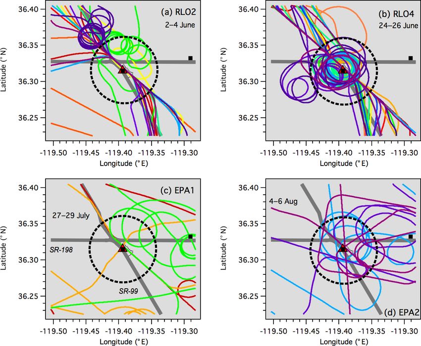
1894                              A. O. Langford et al.: Intercomparison of lidar, aircraft, and surface ozone measurements

Figure 3. Time series plots (local Pacific daylight time, PDT) of
the O3 concentrations retrieved 815 ± 15 m downrange and 27.5 m
above the surface by TOPAZ (black line) with the measurements           Figure 4. (a) A 4-day time series (9–13 June) showing the O3 con-
from the in situ 2B monitor sampling 5 m a.g.l. at the TOPAZ loca-      centrations in air sampled 5 m a.g.l. above the TOPAZ truck at the
tion (gray dots) during the first (a) and second (b) IOPs. The dashed   VMA (gray line) and the O3 mixing ratios at a height of 27.5 ± 5 m
and dotted lines show the 2008 (75 ppbv) and 2015 (70 ppbv) O3          and distance of 815±15 m retrieved from the TOPAZ measurements
NAAQS, respectively.                                                    (filled black circles). The solid black and dotted staircase lines show
                                                                        the 1 h measurements from the Visalia and Hanford regulatory mon-
                                                                        itors. (b) Scatterplot comparing the 27.5 m TOPAZ measurements
profiles around the airport but never directly sampled the ver-         to the interpolated 5 m in situ measurements. The filled gray circles
tical column probed by the lidar. The comparisons were also             (with dotted ODR fit) show the entire CABOTS dataset from Fig. 3,
conducted as brief elements of multi-hour sampling flights              and the filled black circles (with dashed ODR fit) show only those
with other objectives, and time constraints and air traffic con-        measurements made during the day (09:00 to 18:30 PDT) when the
                                                                        winds were southeasterly (125 to 145◦ ) and greater than 2.5 m s−1 .
siderations sometimes contributed to the spatial and temporal
                                                                        The solid line shows the 1 : 1 correspondence.
mismatches. The piston-engine Mooney took about 25 min to
execute an ascending profile from the surface to 3 km, while
the Alpha Jet took about 9 min (similar to the 8 min TOPAZ
                                                                        4.2.1   UC Davis–Scientific Aviation Mooney
integration time) to conduct a descending profile from 3 km
to the surface. Spatial mismatches were also created by the             The RLO flights were executed as a series of 2–3-day de-
vertically smoothing of the DIAL retrieval, which can both              ployments with as many as four flights per day lasting 2 to
smooth and displace sharp vertical concentration gradients              3 h each between Fresno and Bakersfield. Two of these de-
seen by the aircraft. Similar considerations apply to compar-           ployments, RLO2 (2–4 June) and RLO4 (24–26 July), over-
isons between lidars and ozonesondes since balloons have a              lapped with the first and second TOPAZ IOPs, respectively,
finite rise time and can be carried many kilometers down-               and included low approaches at VMA on most of the flights
wind from the launch site (Leblanc et al., 2018). Despite               with spiral profiles near VMA on several. Both deployments
these caveats, we show that the lidar and aircraft measure-             occurred as warm temperatures (> 40 ◦ C) and weak anticy-
ments usually agreed to within ±10 %, the nominal accuracy              clonic winds associated with synoptic high-pressure systems
of ECC ozonesondes in the troposphere (Smit et al., 2014),              resulted in the buildup of surface ozone across the South
which is the generally accepted reference standard for ozone            Coast Air Basin and San Joaquin Valley Air Basin. The high-
profile measurements.                                                   est measured MDA8 O3 in the SJVAB during the first IOP
                                                                        was recorded on 4 June at Clovis (91 ppbv), which lies about
                                                                        65 km northwest of VMA (see Fig. 1b). The highest reported
                                                                        MDA8 O3 during the second IOP (and the year) was recorded
                                                                        on 27 July at Parlier (101 ppbv), which lies midway between

Atmos. Meas. Tech., 12, 1889–1904, 2019                                                     www.atmos-meas-tech.net/12/1889/2019/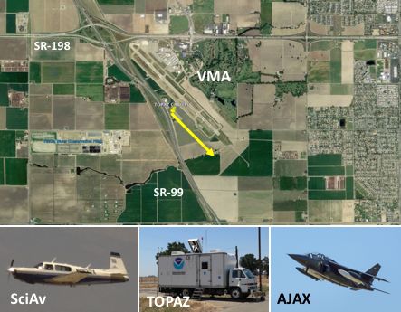
A. O. Langford et al.: Intercomparison of lidar, aircraft, and surface ozone measurements                                        1895

                                                                       the aircraft between the surface and 25 m a.g.l. All of the
                                                                       aircraft measurements lie within 10 % of the O3 retrieved
                                                                       by TOPAZ with the exception of the much higher values
                                                                       (> 100 ppbv) measured by the Mooney around 14:00 PDT on
                                                                       3 June (Fig. 8a; see below). The scatterplots in Fig. 8e and f
                                                                       show that the aircraft also measured much higher concentra-
                                                                       tions than the in situ surface monitor during the night and
                                                                       early morning, in agreement with the lidar measurements
                                                                       in Fig. 4. The differences were smaller on 27 July than on
                                                                       3 June, and also less pronounced than those in Fig. 4. Closer
                                                                       agreement between the aircraft and surface measurements
                                                                       might be expected since some of the aircraft measurements
                                                                       were made within 200 m of the lidar truck (see Fig. 2). The
                                                                       dark blue points show that the low bias in the surface mea-
                                                                       surements decreased during the day after the surface inver-
                                                                       sion had dissipated (there were too few measurements to ef-
                                                                       fectively filter them by wind speed or direction). The mean
Figure 5. Scatterplots with ODR fits comparing the 27.5 m TOPAZ        ODR fit parameters based on the measurements from both
measurements with the 1 h measurements from the regulatory mon-        RLO2 and RLO4 listed in Table 1 are very similar to those
itors at (a) Visalia–N. Church Street, (b) Hanford, (c) Parlier, and   found for the lidar, which suggests that the filtered surface
(d) Porterville. The measurements in the upper box and x axis la-      measurements still have low bias that could be either instru-
bel refer to the distance from the VMA and sampling height above
                                                                       mental or sampling related.
ground, respectively. The Visalia monitor is operated by the Cali-
fornia Air Resources Board. The remaining three are operated by
                                                                          Figure 9 compares the aircraft and lidar O3 measurements
CARB and the SJVAPCD. The TOPAZ measurements are interpo-              made during five of the ascending profiles conducted by the
lated to the 1 h time base of the regulatory measurements for the      Mooney near the VMA. FLT19 was conducted in the early
comparison.                                                            afternoon of 3 June and FLT33, FLT35, FLT36, and FLT37
                                                                       were conducted over the 24 h period beginning just after lo-
                                                                       cal midnight on 25 July. The four consecutive TOPAZ pro-
Clovis and the VMA. The monitors at Visalia and Hanford                files acquired during the time required for the Mooney to
reported MDA8 concentrations of 72 and 88 ppbv, respec-                reach the top of each profile (∼ 15–30 min at a climb rate of
tively, on 4 June, and 83 and 85 ppbv on 27 July. Figure 3             ∼ 2.2 m s−1 ) are plotted in each panel. The gray envelopes
shows that the highest O3 mixing ratios measured by the                show the lidar mean profile ±10 %. The differences between
VMA surface monitor and TOPAZ (27.5 m a.g.l.) were also                consecutive profiles reflect the combined effects of atmo-
recorded on these 2 days.                                              spheric variability and the precision of the lidar measure-
   The flight tracks from all of the Mooney sorties during the         ments.
RLO2 and RLO4 deployments are plotted in Fig. 6a. FLT29                   Overall, the agreement between the TOPAZ and Mooney
(RLO4) was a transit flight from the Scientific Aviation home          profiles in Fig. 9 is within ±10 %, but there are some notable
base near Sacramento to Fresno. The remaining RLO flights              discrepancies. Most of these arise from the coarser vertical
were between Fresno and Bakersfield as noted above. The                resolution of the lidar retrievals, which smooth out abrupt
two EPA deployments (27–29 July and 4–6 August) were of                concentration changes such as those seen at the top of the
longer duration than the RLO flights with morning and af-              boundary layer (∼ 0.8 km a.g.l.) in Fig. 9a and between 2 and
ternoon sorties that placed more emphasis on cross-valley              3 km in Fig. 9e where several narrower layers are smoothed
measurements and transects to the coast (Fig. 6b) includ-              into one broad layer in the lidar profile. Figure 9e also shows
ing profiles above the South Bay (EPA1) and Chews Ridge                that the agreement between the lidar and aircraft measure-
(EPA2). The afternoon flights during both series included              ments is better at low altitudes where the addition of the slant
legs to Visalia.                                                       path measurements significantly improves the effective ver-
   Figure 7 shows the sections of the RLO and EPA flight               tical resolution of the lidar. Fine-scale variability in O3 also
tracks that passed within 5 km of TOPAZ (dashed black cir-             contributes to some of the observed differences, particularly
cles). Most of these flights included low (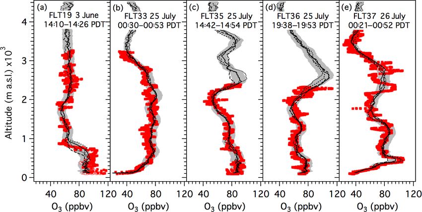
1896                             A. O. Langford et al.: Intercomparison of lidar, aircraft, and surface ozone measurements

Figure 6. (a) Map of the San Joaquin Valley showing the RLO flight tracks coincident with the TOPAZ measurements (RLO2 and RLO4).
The filled black squares show the regulatory surface monitors. The CABOTS sampling sites at CRO and VMA are marked by red triangles.
The other abbreviations are the Fresno (FAT), Visalia (VIS), and Bakersfield (BFL) airport codes. Note that VMA and VIS refer to the same
airport. (b) The same as (a) but with the EPA flight tracks (EPA1 and EPA2).

Figure 7. RLO and EPA flight tracks in the vicinity of TOPAZ. (a) RLO2 (2–4 June), (b) RLO4 (24–26 July), (c) EPA1 (27–29 July), and
(d) EPA2 (4–6 August). Each color represents a different flight. The red triangle with a black square marks the location of TOPAZ at the
VMA and the dashed black circles show the 5 km radius used for the profile comparisons. The lone black square represents the Visalia–N.
Church St. O3 monitor.

   The lidar profiles from 26 July (Fig. 9e) also show large           and the low-altitude “layer” near 400 m in Fig. 9e is actually
profile-to-profile changes in the narrow high O3 layer ly-             a short-lived puff of smoke and elevated O3 from the fire.
ing just above the top of the nocturnal boundary layer (∼              This is more obvious in the expanded view of the profiles
0.3 km a.s.l.). The 25 and 26 July measurements (Fig. 9b–              shown in Fig. 10a. Only two of the four lidar profiles from
e) were made several days after the Soberanes Fire started             Fig. 9e are plotted: the first profile coinciding with the air-

Atmos. Meas. Tech., 12, 1889–1904, 2019                                                   www.atmos-meas-tech.net/12/1889/2019/
A. O. Langford et al.: Intercomparison of lidar, aircraft, and surface ozone measurements                                         1897

Figure 8. (a–d) Time series of the surface in situ O3 (gray dots) and 27.5 m TOPAZ O3 (red line) measured during the RLO and EPA low
approaches on (a) 2–5 June, (b) 24–27 July, (c) 27–30 July, and (d) 4–7 August 2016. The red envelope shows the TOPAZ data ±3 ppbv,
the nominal accuracy of the lidar retrievals. The blue squares represent the 1 s sampled (2 s recorded) Scientific Aviation measurements
made between the surface and 25 m a.g.l. The filled yellow circles in (a) and (c) show 2 s measurements from AJAX low approaches (see
text). Panels (e) and (f) show scatterplots of the in situ surface measurements and the Scientific Aviation data from the RLO flights in
panels (a) and (b), respectively. The ODR fit parameters refer to the dark blue points which represent the measurements from daytime
(08:30–18:30 PDT) flights.

craft measurements (solid trace, ±10 %) and the profile ac-           4.2.2   NASA Alpha Jet Atmospheric eXperiment
quired 16–24 min later when the puff had mostly disappeared                   (AJAX)
(dashed trace). The corresponding lidar backscatter measure-
ments are plotted in Fig. 10b, and Fig. 10c shows the NO2
and H2 O profiles measured by the aircraft. The backscat-             AJAX conducted four research flights over the SJV while
ter measurements show that the TOPAZ retrievals are unaf-             TOPAZ was operational, with two additional flights (21 June
fected by strong backscatter gradients, which can create sec-         and 7 July) between the two IOPs. The Alpha Jet executed
ond derivative-like inflection points in the DIAL O3 profiles         descending spiral profiles from 4 to 5 km down to the sur-
(Kovalev and McElroy, 1994). The absence of a correspond-             face that ended in low approaches on three of these flights:
ing structure in the aircraft NO2 and H2 O profiles confirms          AJX190 on 3 June, AJX191 on 15 June, and AJX195 on
that the high O3 layer seen in the lidar and aircraft mea-            21 July. The aircraft also conducted a very low approach
surements was not an artifact caused by interferences from            (∼ 5 m) at VMA on 28 July (AJX196) but did not execute
these species, which weakly absorb between 280 and 300 nm             a full profile. These low approach measurements are repre-
(Proffitt and Langford, 1997).                                        sented by the filled yellow circles in Fig. 8a and c. The first
                                                                      and last flights (AJX190 and AJX196) coincided with the

www.atmos-meas-tech.net/12/1889/2019/                                                    Atmos. Meas. Tech., 12, 1889–1904, 2019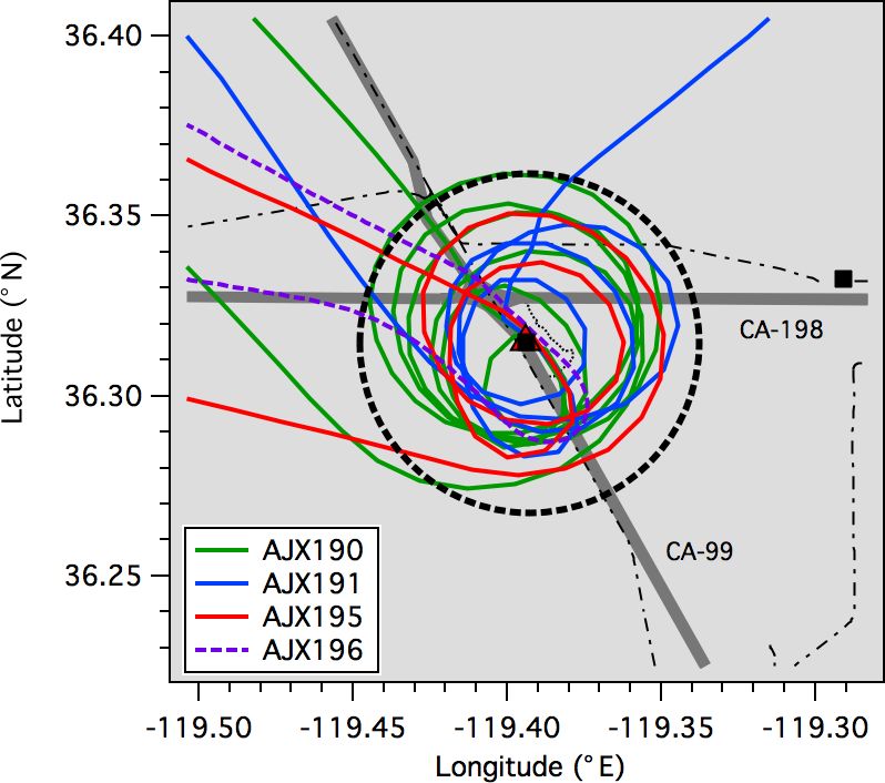
1898 A. O. Langford et al.: Intercomparison of lidar, aircraft, and surface ozone measurements
Figure 9. Profile plots comparing the TOPAZ (black lines) and Scientific Aviation (red squares) O3 measurements on (a) FLT19, 3 June;
(b) FLT33, 25 July; (c) FLT35 25 July; (d) FLT36, 25 July; and (e) FLT37, 26 July. The dotted, short-dashed, solid, and long-dashed lines
show the four consecutive 8 min lidar profiles acquired during the aircraft profiles. The gray envelopes show the mean lidar profile ±10 % as
reference. Note the large variability near the surface and the sharp transition at 800 m in the 3 June aircraft measurements (see Fig. 3a).
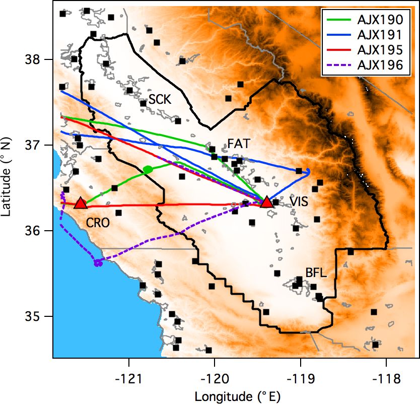
Figures 11 and 12 are similar to Figs. 6 and 7 but in-
stead show the AJAX flight tracks. The first AJAX flight
(AJX190) on 3 June during IOP1 overlapped with the UC
Davis–Scientific Aviation RLO2 deployment. AJX191 took
place about 2 weeks later in IOP1, and AJX195 occurred
several days prior to the RLO4 deployment in IOP2. AJAX
also executed profiles (not shown here) above and upwind of
Chews Ridge on AJX190 and AJX191, near Bodega Bay on
AJX191 and 195, and the Soberanes Fire plume on AJX196.
Figure 13 displays coincident AJAX and TOPAZ profiles
in plots similar to those shown for the Mooney in Fig. 9 but
with an extended vertical axis to reflect the higher range of
these profiles. The points in Fig. 13 are sparser than those in
Fig. 9 in part because of the 10 s averaging time, and in part
because the Alpha Jet executed its descending profiles with
Figure 10. (a) Expanded view of the lidar and aircraft O3 profiles
from Fig. 9e plotted with coincident (b) lidar backscatter and (c) air- an airspeed of about 110 m s−1 compared to about 60 m s−1
craft NO2 and H2 O profiles. The solid black profile (±10 % in gray) for the ascending Mooney profiles.
in (a) shows the lidar profile coinciding with the aircraft measure- The agreement between the Alpha Jet and TOPAZ mea-
ments below 1 km; the dashed black line shows the profile measured surements is within ±10 % on all 3 days except for 3 June
16–24 min later. This is also true for the backscatter profiles in (b). (Fig. 13a), when the measured aircraft and retrieved li-
The horizontal gray band highlights the smoke puff from the Sober- dar concentrations differ by as much as 12 ppbv (20 %) at
anes Fire. 2.5 km a.s.l. and 20 ppbv (∼ 50 %) at 5.2 km a.s.l. The dis-
parities between the inbound and outbound measurements in
Fig. 13a show that the Alpha Jet encountered strong hori-
high-ozone episodes mentioned earlier, and the third flight zontal gradients below 800 m in the boundary layer when it
(AJX195) also occurred during a period of high pressure. The arrived at the VMA about 3 h after the Mooney found sim-
second flight (AJX191) was conducted as a deep closed low ilar horizontal variability (see Figs. 8a and 9a). The Google
moved into the Pacific Northwest, however, bringing unsea- Earth map and latitude–altitude and longitude–altitude plots
sonably cool temperatures (26 ◦ C) and strong surface winds in Fig. 14 better illustrate the extent of the horizontal vari-
to the SJV. This cyclonic system advected a large Asian pol- ability in the boundary layer. These figures also show weaker
lution plume across the valley in the middle troposphere, but horizontal gradients above 3 km where the disagreement be-
surface ozone remained low with the peak MDA8 O3 concen- tween the lidar and aircraft is most pronounced.
tration in the SJVAB only reaching 59 ppbv at the Sequoia–
Kings Canyon monitor.
Atmos. Meas. Tech., 12, 1889–1904, 2019 www.atmos-meas-tech.net/12/1889/2019/A. O. Langford et al.: Intercomparison of lidar, aircraft, and surface ozone measurements 1899
Table 1. Summary of the lidar, surface, and aircraft comparisons.
A B Ratio ±1σ (A/B) Diff. ±1σ (A-B) Slope∗ (A vs. B) Int.∗ (A vs. B)
TOPAZ VMA 1.06 ± 0.08 2.9 ± 3.7 ppbv 1.00 ± 0.03 −2.6 ± 1.5 ppbv
SciAv VMA 1.07 ± 0.10 5.0 ± 5.0 ppbv 1.01 ± 0.01 −4.5 ± 1.1 ppbv
TOPAZ SciAv 1.01 ± 0.04 0.8 ± 2.8 ppbv 1.00 ± 0.13 1.0 ± 9.0 ppbv
TOPAZ AJAX 1.08 ± 0.06 4.2 ± 0.8 ppbv 1.07 ± 0.13 1.8 ± 3.4 ppbv
∗ From orthogonal distance regression (ODR) fits. Uncertainties are 95 % confidence limits.
Figure 12. AJAX flight tracks in the vicinity of the VMA (red tri-
angle with a black square). The lone black square represents the
Figure 11. Map of the San Joaquin Valley showing the AJAX flight
Visalia–N. Church St. O3 monitor and the dashed black circle marks
tracks on 3 June (AJX190), 15 June (AJX191), 21 July (AJX195),
the 5 km radius window used for the profile comparisons. The heavy
and 28 July (AJX196). The abbreviations and symbols are the same
gray lines show the major highways and the black dotted–dashed
as in Fig. 6.
lines the railroads.
5 Discussion lidar retrievals and aircraft measurements, with the effective
temporal averaging of the AJAX and SciAv measurements
The results of the different O3 comparisons are summarized increasing to about 2 and 4 min, respectively. Each point in
in Table 1. As was noted above, comparisons between the the scatterplots of Fig. 15a and b represents the mean mixing
lidar and aircraft profiles are subject to uncertainties arising ratio from one of these 1 km segments, with the error bars
from sampling differences introduced by the intrinsic verti- showing the standard deviation of the mean. The intercepts
cal smoothing of the lidar retrievals and horizontal displace- and slopes derived from orthogonal distance regressions of
ments between the aircraft and lidar. The potential impact both datasets overlap with zero and unity, respectively, within
of horizontal displacements on the comparisons when the the 95 % confidence limits of the ODR fits. The lower panels
O3 spatial variability is large is illustrated by Fig. 14, and a (Fig. 15c and d) plot the same data as differences which show
good example of the differences created by the lidar smooth- that the TOPAZ and SciAv measurements (Fig. 15c) agree to
ing is seen near the top of the boundary layer around 0.8 km within 1 ppbv on average, and the TOPAZ and AJAX mea-
in Fig. 9a. These uncertainties can be reduced by averaging surements (Fig. 15d) to within 4.2 ppbv. Neither plot shows
the measurements to be compared over larger volumes. Fig- evidence of a systematic altitude dependence in the differ-
ure 15 compares the lidar and aircraft measurements from ences.
the profiles plotted in Figs. 9 and 13, and from several other Both lidar–aircraft comparisons are limited by the small
RLO and EPA flights not shown, with each individual pro- number of common measurements with only three profiles
file averaged over 1 km segments (0 to 1 km, 1 to 2 km, etc.). available for the AJAX comparisons. The SciAv comparisons
This averaging decreases the influence of O3 spatial variabil- include data from seven flights, but only the five profiles
ity and also reduces the statistical uncertainties in both the shown in Fig. 9 extend above 2 km and only three of those
www.atmos-meas-tech.net/12/1889/2019/ Atmos. Meas. Tech., 12, 1889–1904, 20191900 A. O. Langford et al.: Intercomparison of lidar, aircraft, and surface ozone measurements
Figure 13. Profile plots comparing the TOPAZ (black lines) and
10 s AJAX (red squares) measurements on (a) AJX190, 3 June;
(b) AJX191, 15 June; and (c) AJX195, 21 July. The closed squares
correspond to the Alpha Jet descent and the open squares the subse-
quent climb out. Note the differences between these measurements.
The dotted, dashed, and solid lines show the order of the three 8 min
lidar profiles that bracket the AJAX profile. The gray envelopes
show the mean lidar profile ±10 % as reference. The significance
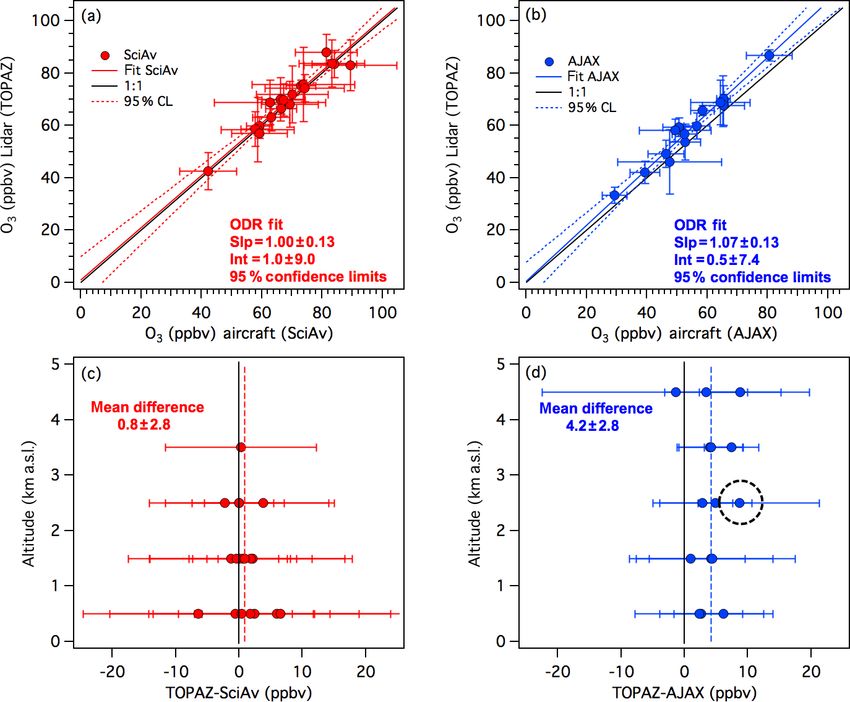
Figure 15. (a, b) Scatterplots comparing the TOPAZ lidar retrievals
of the dashed oval in (b) is discussed in the text.
to in situ O3 measurements from seven SciAv Mooney and three
NASA Alpha Jet flights, respectively, averaged over 1 km vertical
bins. The error bars show the standard deviations of the 1 km col-
umn means. (c, d) Differences between the 1 km mean TOPAZ and
aircraft measurements from (a) and (b) plotted as a function of al-
titude. The vertical dashed lines show the mean differences. The
dashed circle in (d) corresponds to the dashed oval in Fig. 13b (see
text).
reach 3 km. These limited datasets make the comparisons
more sensitive to the influence of individual points. For ex-
ample, the point surrounded by the dashed circle in Fig. 15d
includes the measurements from within the dashed oval in
Fig. 13b where the lidar retrieval is clearly smoothing out
the vertical gradient compared to the aircraft measurements.
If this measurement point is excluded, the mean TOPAZ–
AJAX difference decreases to 3.9±2.6. In either case, the dif-
ferences between the TOPAZ lidar retrievals and the in situ
surface and aircraft measurements lie within the combined
uncertainties of the different measurements and well within
the 10 % accuracy standard set by the ECC ozonesonde.
6 Summary and conclusions
The lidar, aircraft, and ozonesonde profiles acquired during
Figure 14. (a) Google Earth image of the TOPAZ and AJAX pro- the 2016 CABOTS field campaign provide an unprecedented
files from 3 June 2016 showing the spatial variations across the
look at the vertical distribution of lower tropospheric O3
∼ 8 km diameter spiral profile by the Alpha Jet during its descent
above California during late spring and summer. The good
and climb out over the VMA. (b, c) AJAX and TOPAZ profiles from
Fig. 13a plotted as a function of latitude (b) and longitude (c). Both agreement between the low-elevation TOPAZ measurements
plots are 10 km wide. Note the strong horizontal gradients below and the collocated and regional (< 45 km) surface monitors
1.2 km. suggests that the measurements made at the VMA during
CABOTS can be considered representative of the central San
Joaquin Valley. Comparisons between the NOAA TOPAZ li-
dar profiles and the surface and aircraft measurements agree
Atmos. Meas. Tech., 12, 1889–1904, 2019 www.atmos-meas-tech.net/12/1889/2019/A. O. Langford et al.: Intercomparison of lidar, aircraft, and surface ozone measurements 1901
The CABOTS ozonesondes were launched too far away
(> 300 km) from the VMA to allow quantitative compar-
isons with the lidar. However, TOPAZ was relocated to the
NASA Jet Propulsion Laboratory (JPL) Table Mountain Fa-
cility (TMF) in the San Gabriel Mountains immediately af-
ter CABOTS for the Southern California Ozone Observa-
tion Project (SCOOP), a multiple lidar and ozonesonde inter-
comparison organized by the NASA-sponsored Tropospheric
Ozone Lidar Network or TOLNet (https://www-air.larc.nasa.
gov/missions/TOLNet/, last access: 18 March 2019) at the
NASA JPL TMF (Leblanc et al., 2018). The results from
the SCOOP intercomparison and those presented here com-
plete the inter-validation of the CABOTS lidar, aircraft, and
ozonesonde profile measurements.
Data availability. CARB provided surface monitoring data (avail-
able at: https://www.arb.ca.gov/aqmis2/aqdselect.php, CARB,
2019). NOAA provided TOPAZ ozone lidar data (available at:
https://www.esrl.noaa.gov/csd/groups/csd3/measurements/cabots/
topaz.php, NOAA, 2019). NASA provided the AJAX aircraft
data (available at: https://www.esrl.noaa.gov/csd/groups/csd3/
measurements/cabots/ajax.php, NASA, 2019). UC Davis provided
the Scientific Aviation aircraft data (available at: https://www.esrl.
noaa.gov/csd/groups/csd3/measurements/cabots/ucdavis/Aircraft/,
UC Davis, 2019).
Figure 16. Time–height curtain plots of the TOPAZ ozone mea-
surements from (a) 25 to 26 July with the Scientific Aviation pro- Competing interests. The authors declare that they have no conflict
files from FLT35, FLT36, and FLT37 superimposed and (b) 15 June of interest.
with the coincident AJAX profile superimposed. The aircraft mea-
surements made within 5 km of VMA (arrows) are highlighted by
squares and colorized using the same scale as the TOPAZ data. The Acknowledgements. The California Baseline Ozone Transport
high O3 layers around 3 km a.s.l. in (a) are related to the Soberanes Study (CABOTS) field measurements described here were funded
Fire; the measurements plotted in the lower right corner of (a) cor- by the California Air Resources Board (CARB) under contract
respond to the data shown in Fig. 10. nos. 15RD012 (NOAA ESRL), 14-308 (UC Davis), and 17RD004
(NASA Ames). We would like to thank Jin Xu and Eileen McCauley
of CARB for their support and assistance in the planning and ex-
ecution of the project and are grateful to the CARB and the San
within the stated uncertainties, and we conclude that all of Joaquin Valley Unified Air Pollution Control District (SJVAPCD)
these O3 measurements may be used with confidence. personnel who provided logistical support during the execution of
The coordinated lidar and aircraft sampling of O3 above the field campaign. We would also like to thank Cathy Burgdorf-
the central San Joaquin Valley during CABOTS also illus- Rasco of NOAA ESRL and CIRES for maintaining the CABOTS
trates the synergy between the two types of measurements. data site. The NOAA team would also like to thank Ann Weick-
Lidar can provide long time series of the O3 (and backscatter) mann, Scott Sandberg, and Richard Marchbanks for their assis-
vertical distributions above a fixed location while the aircraft tance during the field campaign. The NOAA-ESRL lidar opera-
can place the lidar measurements within a larger spatial con- tions were also supported by the NOAA Climate Program Office,
text and measure other important parameters. This synergy Atmospheric Chemistry, Carbon Cycle, and Climate (AC4) Pro-
gram and the NASA-sponsored Tropospheric Ozone Lidar Network
is illustrated by the two time–height curtain plots displayed
(TOLNet, http://www-air.larc.nasa.gov/missions/TOLNet/, last ac-
in Fig. 16. Figure 16a shows the continuous TOPAZ mea- cess: 18 March 2019). The UC Davis–Scientific Aviation measure-
surements from a 14 h time span on 25–26 July with the data ments were also supported by the U.S. Environmental Protection
from SciAv FLT35, FLT36, and FLT37 superimposed. The Agency and Bay Area Air Quality Management District through
aircraft measurements made within 5 km of VMA are high- contract no. 2016-129. Ian C. Faloona was also supported by the
lighted by colored squares outlined in white. Figure 16b is California Agricultural Experiment Station, hatch project CA-D-
similar but shows 10 h of continuous TOPAZ measurements LAW-2229-H. The NASA AJAX project was also supported with
from 15 June with the AJAX measurements (AJX191) super- Ames Research Center director’s funds, and the support and part-
imposed. nership of H211, LLC is gratefully acknowledged. Josette E. Mar-
www.atmos-meas-tech.net/12/1889/2019/ Atmos. Meas. Tech., 12, 1889–1904, 20191902 A. O. Langford et al.: Intercomparison of lidar, aircraft, and surface ozone measurements
rero and Ju-Mee Ryoo were supported through the NASA Postdoc- CARB: Surface monitoring data, available at: https://www.arb.ca.
toral Program, and Mimi E. McNamara was funded through the gov/aqmis2/aqdselect.php, last access: 18 March 2019.
Center for Applied Atmospheric Research and Education (NASA Hamill, P., Iraci, L. T., Yates, E. L., Gore, W., Bui, T. P., Tanaka, T.,
MUREP). The views, opinions, and findings contained in this re- and Loewenstein, M.: A New Instrumented Airborne Platform
port are those of the author(s) and should not be construed as an for Atmospheric Research, B. Am. Meteorol. Soc., 97, 397–404,
official National Oceanic and Atmospheric Administration or U.S. https://doi.org/10.1175/Bams-D-14-00241.1, 2016.
Government position, policy, or decision. Jaffe, D. A., Cooper, O. R., Fiore, A. M., Henderson, B. H., Ton-
neson, G. S., Russell, A. G., Henze, D. K., Langford, A. O., Lin,
M., and Moore, T.: Scientific assessment of background ozone
Review statement. This paper was edited by Folkert Boersma and over the U.S.: Implications for air quality management, Elem.
reviewed by two anonymous referees. Sci. Anth., 6, 56, https://doi.org/10.1525/elementa.309, 2018.
Johnson, B. J., Oltmans, S. J., Vomel, H., Smit, H. G. J.,
Deshler, T., and Kroger, C.: Electrochemical concentration
cell (ECC) ozonesonde pump efficiency measurements and
tests on the sensitivity to ozone of buffered and unbuffered
References ECC sensor cathode solutions, J. Geophys. Res., 107, 4393,
https://doi.org/10.1029/2001jd000557, 2002.
Alvarez, R. J., II, Senff, C. J., Langford, A. O., Weickmann, A. Kempfer, U., Carnuth, W., Lotz, R., and Trickl, T.: A Wide-Range
M., Law, D. C., Machol, J. L., Merritt, D. A., Marchbanks, Ultraviolet Lidar System for Tropospheric Ozone Measurements
R. D., Sandberg, S. P., Brewer, W. A., Hardesty, R. M., and – Development and Application, Rev. Sci. Instrum., 65, 3145–
Banta, R. M.: Development and Application of a Compact, 3164, https://doi.org/10.1063/1.1144769, 1994.
Tunable, Solid-State Airborne Ozone Lidar System for Bound- Kovalev, V. A. and McElroy, J. L.: Differential Absorption Li-
ary Layer Profiling, J. Atmos. Ocean Tech., 28, 1258–1272, dar Measurement of Vertical Ozone Profiles in the Troposphere
https://doi.org/10.1175/Jtech-D-10-05044.1, 2011. That Contains Aerosol Layers with Strong Backscattering Gra-
Ancellet, G. and Ravetta, F.: Analysis and validation dients – a Simplified Version, Appl. Optics, 33, 8393–8401,
of ozone variability observed by lidar during the https://doi.org/10.1364/Ao.33.008393, 1994.
ESCOMPTE-2001 campaign, Atmos. Res., 74, 435–459, Lagarias, J. S. and Sylte, W. W.: Designing and Man-
https://doi.org/10.1016/j.atmosres.2004.10.003, 2005. aging the San Joaquin Valley Air-Quality Study,
Asher, E. C., Christensen, J. N., Post, A., Perry, K., Cliff, S. S., J. Air Waste Manage. Assoc., 41, 1176–1179,
Zhao, Y. J., Trousdell, J., and Faloona, I.: The Transport of Asian https://doi.org/10.1080/10473289.1991.10466912, 1991.
Dust and Combustion Aerosols and Associated Ozone to North Langford, A. O., Senff, C. J., Alvarez, R. J., Banta, R. M., and
America as Observed From a Mountaintop Monitoring Site in the Hardesty, R. M.: Long-range transport of ozone from the Los
California Coast Range, J. Geophys. Res.-Atmos., 123, 5667– Angeles Basin: A case study, Geophys. Res. Lett., 37, L06807,
5680, https://doi.org/10.1029/2017jd028075, 2018. https://doi.org/10.1029/2010gl042507, 2010.
Avnery, S., Mauzerall, D. L., Liu, J. F., and Horowitz, L. W.: Global Langford, A. O., Senff, C. J., Alvarez, R. J., Banta, R. M., Hardesty,
crop yield reductions due to surface ozone exposure: 2. Year R. M., Parrish, D. D., and Ryerson, T. B.: Comparison between
2030 potential crop production losses and economic damage un- the TOPAZ Airborne Ozone Lidar and In Situ Measurements
der two scenarios of O-3 pollution, Atmos. Environ., 45, 2297– during TexAQS 2006, J. Atmos. Ocean. Tech., 28, 1243–1257,
2309, https://doi.org/10.1016/j.atmosenv.2011.01.002, 2011a. https://doi.org/10.1175/Jtech-D-10-05043.1, 2011.
Avnery, S., Mauzerall, D. L., Liu, J. F., and Horowitz, L. Langford, A. O., Brioude, J., Cooper, O. R., Senff, C. J., Alvarez,
W.: Global crop yield reductions due to surface ozone R. J., Hardesty, R. M., Johnson, B. J., and Oltmans, S. J.: Strato-
exposure: 1. Year 2000 crop production losses and spheric influence on surface ozone in the Los Angeles area dur-
economic damage, Atmos. Environ., 45, 2284–2296, ing late spring and early summer of 2010, J. Geophys. Res., 117,
https://doi.org/10.1016/j.atmosenv.2010.11.045, 2011b. D00V06, https://doi.org/10.1029/2011JD016766, 2012.
Bao, J. W., Michelson, S. A., Persson, P. O. G., Djalalova, I. Langford, A. O., Senff, C. J., Alvarez, R. J., Brioude, J., Cooper,
V., and Wilczak, J. M.: Observed and WRF-simulated low- O. R., Holloway, J. S., Lin, M. Y., Marchbanks, R. D., Pierce,
level winds in a high-ozone episode during the Central Cali- R. B., Sandberg, S. P., Weickmann, A. M., and Williams,
fornia Ozone Study, J. Appl. Meteorol. Clim., 47, 2372–2394, E. J.: An overview of the 2013 Las Vegas Ozone Study
https://doi.org/10.1175/2008jamc1822.1, 2008. (LVOS): Impact of stratospheric intrusions and long-range trans-
Beekmann, M., Ancellet, G., Martin, D., Abonnel, C., Duveerneuil, port on surface air quality, Atmos. Environ., 109, 305–322,
G., Eideliman, F., Bessemoulin, P., Fritz, N., and Gizard, E.: In- https://doi.org/10.1016/J.Atmosenv.2014.08.040, 2015.
tercomparison of tropospheric ozone profiles obtained by elec- Leblanc, T., Brewer, M. A., Wang, P. S., Granados-Muñoz, M.
trochemical sondes, a ground based lidar and an airborne UV- J., Strawbridge, K. B., Travis, M., Firanski, B., Sullivan, J. T.,
photometer, Atmos. Environ., 29, 1027–1042, 1995. McGee, T. J., Sumnicht, G. K., Twigg, L. W., Berkoff, T. A.,
Brune, W. H., Baier, B. C., Thomas, J., Ren, X., Cohen, R. C., Carrion, W., Gronoff, G., Aknan, A., Chen, G., Alvarez, R. J.,
Pusede, S. E., Browne, E. C., Goldstein, A. H., Gentner, D. Langford, A. O., Senff, C. J., Kirgis, G., Johnson, M. S., Kuang,
R., Keutsch, F. N., Thornton, J. A., Harrold, S., Lopez-Hilfiker, S., and Newchurch, M. J.: Validation of the TOLNet lidars: the
F. D., and Wennberg, P. O.: Ozone production chemistry in Southern California Ozone Observation Project (SCOOP), At-
the presence of urban plumes, Faraday Discuss., 189, 169–189,
https://doi.org/10.1039/c5fd00204d, 2016.
Atmos. Meas. Tech., 12, 1889–1904, 2019 www.atmos-meas-tech.net/12/1889/2019/You can also read