Probing Europa's interior with natural sound sources
←
→
Page content transcription
If your browser does not render page correctly, please read the page content below
Icarus 165 (2003) 144–167
www.elsevier.com/locate/icarus
Probing Europa’s interior with natural sound sources
Sunwoong Lee,a Michele Zanolin,a Aaron M. Thode,a Robert T. Pappalardo,b
and Nicholas C. Makris a,∗
a Department of Ocean Engineering, Massachusetts Institute of Technology, 77 Massachusetts Avenue, Room 5-222, Cambridge, MA 02139, USA
b Laboratory for Atmospheric and Space Physics, University of Colorado, Campus Box 392, Boulder, CO 80309-0392, USA
Received 24 December 2002; revised 26 April 2003
Abstract
Europa’s interior structure may be determined by relatively simple and robust seismo-acoustic echo sounding techniques. The strategy is
to use ice cracking events or impacts that are hypothesized to occur regularly on Europa’s surface as sources of opportunity. A single passive
geophone on Europa’s surface may then be used to estimate the thickness of its ice shell and the depth of its ocean by measuring the travel
time of seismo-acoustic reflections from the corresponding internal strata. Quantitative analysis is presented with full-field seismo-acoustic
modeling of the Europan environment. This includes models for Europan ambient noise and conditions on signal-to-noise ratio necessary for
the proposed technique to be feasible. The possibility of determining Europa’s ice layer thickness by surface wave and modal analysis with
a single geophone is also investigated.
2003 Elsevier Inc. All rights reserved.
Keywords: Europa, interiors; Ices; Tides; Tectonics; Ocean; Acoustic, seismic
1. Introduction energetic for its reflections to stand above the ambient noise
generated by other more distant or less energetic events.
Our goal is to show how Europa’s interior structure may To help quantitatively explore the issues involved in echo-
be revealed by relatively simple and robust seismo-acoustic sounding, and other seismo-acoustic techniques for probing
echo-sounding techniques using natural sources of opportu- Europa’s interior, our analysis proceeds together with the de-
nity. Echo sounding is the traditional and most widely used velopment of a full-field seismo-acoustic model for Europa.
tool to chart the depth and composition of terrestrial oceans This includes analysis of ice-cracking and impact source
and sub-ocean layers (Medwin and Clay, 1998). It employs events, seismo-acoustic propagation in Europa’s stratified
an active acoustic source and passive receiver to measure the environment, and Europan ambient noise. Here we follow
arrival time and amplitude of reflections from the layers to be the common convention of referring to both compressional
charted. Our Europan strategy differs from the terrestrial one and shear wave disturbances in solids, such as Europa’s outer
in that the primary source of sound is not controlled. Rather, ice shell and interior mantle, as “seismic waves,” and com-
it is proposed to arise from ice cracking events and impacts pressional waves in fluids, such as Europa’s potential ocean,
hypothesized to occur regularly on Europa’s surface. A sin- as “acoustic waves.” By this convention, waves that prop-
gle passive geophone on Europa’s surface may then be used agate from ice to water or vice-versa, for example, are re-
ferred to as “seismo-acoustic waves.”
to estimate (1) its range from a natural source event by analy-
Our interest in this problem stems from the significant
sis of direct compressional and shear wave arrivals in the ice,
amount of evidence collected by the Galileo Probe in the
and (2) the thickness of the ice shell and depth of the ocean
past decade to support the possibility that an ocean of liquid
by travel time analysis of specular reflections from the cor-
water may lie beneath Europa’s exterior icy surface. Induced
responding internal strata. The technique, however, requires
magnetic field measurements (Khurana et al., 1998) suggest
the ice-crack or impact event of opportunity to be sufficiently
the existence of a conducting layer beneath the ice surface
that is at least a few kilometers thick and likely corresponds
* Corresponding author. to a liquid ocean of salty water. Various researchers have
E-mail address: makris@mit.edu (N.C. Makris). argued that many of the morphological features that char-
0019-1035/$ – see front matter 2003 Elsevier Inc. All rights reserved.
doi:10.1016/S0019-1035(03)00150-7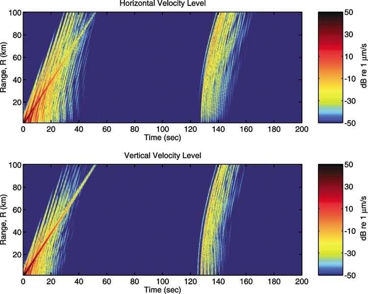
Probing Europa’s interior with natural sound sources                                   145

acterize Europa’s icy surface can best be explained by the                may lead to the near daily formation of cycloidal arcs similar
presence of an ocean of liquid water below (Pappalardo et                 to those observed to extend over hundreds of kilometers on
al., 1998). This is put in context by the conclusion of Ander-            Europa’s surface. Based on the maximum tidal surface stress
son et al. (1998) that the total thickness of ice and potentially         expected by Hoppa et al. (1999) and basic concepts from
liquid water on Europa’s surface is between 80 to 170 km,                 fracture mechanics, we show that a given cycloidal arc is
based on gravity data. Together these observations provide                likely to be formed as a sequence of hundreds of discrete
compelling but inconclusive evidence for a subsurface Eu-                 and temporally disjoint cracking events.
ropan ocean leaving the thickness of the outer ice shell and                  A combination of factors, such as the interplay of diur-
the depth of the potential ocean poorly constrained.                      nal stresses with inhomogeneities in the outer ice shell or
    A variety of techniques have been proposed to measure                 its potential asynchronous rotation due to an ocean layer be-
the thickness of Europa’s outer ice shell. They involve mea-              low (Leith and McKinnon, 1996), may lead to “Big Bang”
surement of crater morphology (Schenk, 2002), tidal grav-                 cracking events. These events would be statistically less fre-
ity (Greenberg, 2002; Anderson et al., 1998; Wu et al.,                   quent but much more energetic than those primarily caused
2001), laser altimetry (Cooper et al., 2002), ice-penetrating             by diurnal stresses in pure ice. Echo returns from Big Bang
radar reflections (Chyba et al., 1998; Moore, 2000), and ice-             events would be more likely to stand above the ambient
bourne seismic wave interference and dispersion (Kovach                   noise and so make echo sounding for Europa’s interior struc-
and Chyba, 2001). All but the last have the advantage of be-              ture more practical. We determine the tensile stresses and
ing achievable by either fly-by or orbital rather than landing            crack depths necessary to generate Big Bang events. We
missions. While each may indicate the presence of an ocean,               also show that even small impactors, in the 1–10-m radius
none are sensitive to its thickness (Cooper et al., 2002).                range, fall into the Big Bang category, and that Big Bang
    Only two techniques are currently available to remotely               events will radiate spectral energy peaking in the roughly 1-
determine the thickness of a deep ocean layer on Europa.                  to 10-Hz range. This is significant because the correspond-
The first involves extensive magnetometer measurements by                 ing seismo-acoustic wavelengths in ice and water will range
a low flying orbiter (Khurana et al., 1998; Kivelson et al.,              from hundreds to thousands of meters. Such long wavelength
1999, 2000). These measurements, however, cannot deter-                   disturbances suffer minimal attenuation from mechanical re-
mine the location of the ocean layer or its structure. The                laxation mechanisms in ice and water and are relatively in-
other is the echo-sounding technique under discussion, the                sensitive to shadowing by similarly sized anomalies in the
primary advantage of which is its ability to determine the ab-            ice or on the seafloor that could severely limit remote sens-
solute interior structure of both the ice and potential ocean             ing techniques that rely on shorter wavelengths.
layers. A potential disadvantage is that it requires a landing
mission.
    The first Europan landing mission will likely carry only              2. Modeling Europa as a stratified seismo-acoustic
a single triaxial geophone capable of measuring seismo-                   medium
acoustic displacements in three spatial dimensions at a single
point on Europa’s surface. Besides echo-sounding, listening                  We begin our analysis by establishing models for Europa
for audible signs of life, and potentially inferring and cat-             as a stratified medium for seismo-acoustic wave propaga-
egorizing dynamical processes of the ice by their acoustic                tion. These models specify compressional wave speed cp ,
signatures, an initial task for this sensor could be to deter-            shear wave speed cs , compressional wave attenuation αp ,
mine the overall level of seismo-acoustic activity on Europa              shear wave attenuation αs , and density ρ as a function of
by time series and spectral analysis. Correlations could be               depth on Europa.
made of ambient noise versus environmental stress level to                   There are two canonical models of Europa’s interior
determine whether noise levels respond directly to orbital ec-            structure. The first is the rigid ice shell model, where heat
centricities. Such an analysis was conducted for the Earth’s              transport is achieved by conduction throughout a completely
Arctic Ocean where roughly two meters of nearly continu-                  brittle and elastic ice-shell (Ojakangas and Stevenson, 1989;
ous pack ice cover an ocean that is typically between 0.1                 Greenberg et al., 1998). The second is the convective ice
and 5 km in depth. These terrestrial results show a near                  shell model, where heat is transported primarily by convec-
perfect correlation between underwater noise level and en-                tion of warm ice at the base that can become buoyant enough
vironmental stresses and moments applied to the ice sheet                 to rise toward the surface (Pappalardo et al., 1998; McKin-
from wind, current, and drift (Makris and Dyer 1986, 1991).               non, 1999; Deschamps and Sotin, 2001).
Additionally, in the Antarctic, both the flexural motion of                  Linearized internal temperature profiles for these two
ice shelves and the level of seismicity due to tidally induced            models are shown in Fig. 1(a). The resulting temperature
ice-fracturing events are correlated with the sea tide (Robin,            profiles are used to construct compressional and shear wave
1958).                                                                    speed profiles in the ice by the methods described in Appen-
    For Europa, Hoppa et al. (1999) show that environmental               dix A. The rigid ice shell model is characterized by an almost
stresses due to tidal forces vary significantly over the period           linear temperature change from the top of the ice shell to the
of its eccentric 3.5 day orbital period and that these stresses           ice–water interface, whereas the convective ice shell model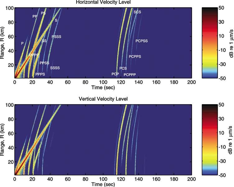
146                                                      S. Lee et al. / Icarus 165 (2003) 144–167

Table 1
Seismo-acoustic parameters
Material                         cp (m/s)                            cs (m/s)                  αp (dB/λ)          αs (dB/λ)            ρ (kg/m3 )
Ice                          see Appendix A                      see Appendix A                      0.24           0.72                  930
Water                  see Chen and Millero (1977)                                                   0.01                                1000
Sediment                          1575                                  80                           1.0            1.5                  1050
Basalt                            5250                                 2500                          0.1            0.2                  2700

                                                                                 20-km rigid, 20-km convecting, and 50-km convecting ice
                                                                                 shell models. The assumed compressional and shear wave
                                                                                 speed profiles through the ice, water and mantle are shown in
                                                                                 Fig. 1(b) and (c) for both 20-km models. Assumed seismo-
                                                                                 acoustic parameters of the medium common to all models
                                                                                 are shown in Table 1.
                                                                                    Attenuation increases significantly with frequency in ter-
                                                                                 restrial sea ice, water and sediment. The attenuation values
                                                                                 shown in Table 1, given in standard decibel units per wave-
                                                                                 length, are valid in the roughly 1–4-Hz range of the spectral
                                                                                 peak of a hypothesized Big Bang ice-quake event used in
                                                                                 the simulations to follow. Ice attenuation values are extrap-
                                                                                 olated to below 200 Hz from the linear trend observed in
                                                                                 Arctic Ocean ice (McCammon and McDaniel, 1985). Atten-
                                                                                 uation due to volumetric absorption in a potential Europan
                                                                                 ocean is taken to be similar to that in terrestrial seawater,
                                                                                 which is relatively insignificant in the low frequency range
                                                                                 of interest in the present study (Urick, 1983). Attenuations
Fig. 1. Temperature, compressional wave speed, and shear wave speed pro-         in the sediment and basalt assumed for the mantle also fol-
files for 20 km thick rigid and convective ice shell models. The solid and
dashed lines represent the rigid and convective ice shell models, respec-
                                                                                 low terrestrial analogs which are far more significant than
tively.                                                                          that found in seawater.
                                                                                    A schematic of Europa as a stratified seismo-acoustic
                                                                                 medium is given in Fig. 2 for a convective ice shell. In the
leads to a strong temperature gradient on top and bottom of
                                                                                 rigid ice shell, the upper thermal boundary layer would con-
the ice shell, and a mild temperature gradient in the middle.
                                                                                 tinue to the ice-ocean interface, eliminating the other two ice
In the latter, temperature is assumed to increase with depth
                                                                                 layers shown.
from an average surface value of 100 K (Orton et al., 1996;
Spencer et al., 1999) to 250 K in the upper thermal bound-
ary layer, which is assumed to comprise the upper 20% of
                                                                                 3. Source mechanisms and characteristics
the ice shell, remain constant for the bulk of ice shell before
finally increasing to 260 K in the lower thermal boundary
layer, which is assumed to comprise the lower 10% of the                             Our primary interest is in source events that are both
ice shell.                                                                       energetic enough and frequent enough for the proposed
   The sound speed of sea water is mainly a function of tem-                     echo-sounding technique to be feasible within the period of
perature, pressure, and salinity. Several regression equations                   a roughly week to month long Europan landing mission.
are available to estimate sound speed from these variables.                      Source events of opportunity must have sufficient energy
Here we employ one valid under high pressure (Chen and                           for their echo returns from the ice–water and water–mantle
Millero, 1977) to estimate the sound speed profile in a sub-                     interfaces to stand above the accumulated ambient noise
surface Europan ocean. This ocean is assumed to have a                           of other more distant or weaker sources. We proceed by
salinity of roughly 3.5%, similar to terrestrial oceans (Khu-                    first estimating the seismo-acoustic energy spectrum of ice-
rana et al., 1998), and a temperature of roughly 273 K, the                      cracking sources and then impact sources.
melting temperature of ice in the terrestrial environment.
   The mantle beneath the ocean is assumed to be comprised                       3.1. Ice-cracking
of a 2-km of sediment layer overlying a basalt halfspace. The
sediment is taken to have sound speed and density similar to                         Surface cracking events are expected to occur in the brit-
water as in terrestrial oceans.                                                  tle, elastic layer of Europa’s outer ice shell in response to
   In our subsequent simulations and analysis, we consider                       tensile stresses arising from a diverse set of mechanisms. We
four Europan sound speed profiles based upon 5-km rigid,                         show that the source time dependence and energy spectrum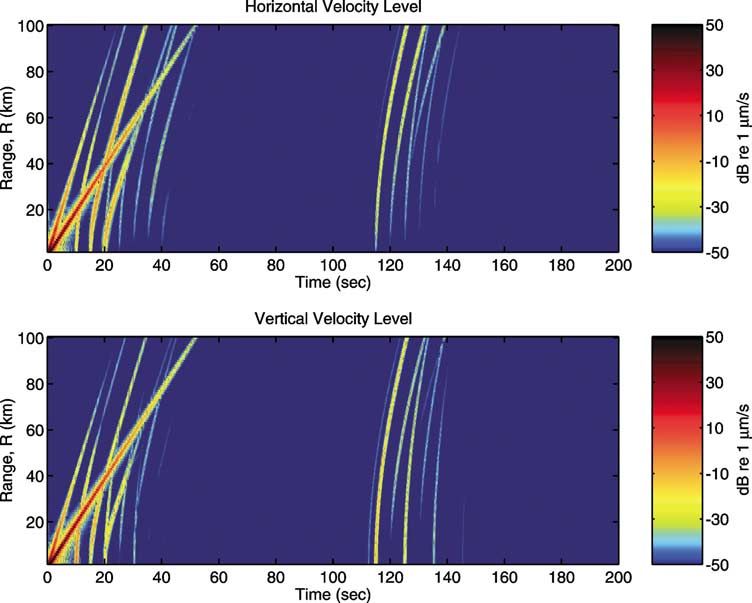
Probing Europa’s interior with natural sound sources                                                147

                                                                                  Fig. 3. The geometry of surface tensile cracks. A crack with depth h prop-
                                                                                  agates until the opening length is h. D0 is the opening width of a crack.
                                                                                  The volume within the dotted line is the regime where the tensile stress is
                                                                                  released by the crack.

                                                                                  40 kPa computed for Europa by Hoppa et al. (1999). This
                                                                                  is higher than the terrestrial value which usually varies be-
                                                                                  tween 1 to 15%. The flexural strength of ice on Europa’s
                                                                                  surface is expected to be higher than that on Earth due to Eu-
                                                                                  ropa’s much lower surface temperature. However, by assum-
                                                                                  ing that flexural strength is proportional to Young’s modulus
                                                                                  and considering Appendix A, the flexural strength will only
                                                                                  increase by roughly 20% which still puts the brine volume
Fig. 2. Schematic diagram of the full Europa model for a convective ice           estimated to be roughly 23% on Europa’s surface.
shell. In the wave speed profile, cp , cs are compressional and shear wave
speeds in elastic media, cw is the acoustic wave speed in the ocean, a is the
                                                                                     The most frequent type of cracking events, expected to
sound speed gradient in the ocean. H and Hw are the thicknesses of the ice        occur daily with the diurnal tide, should then penetrate to
shell and subsurface ocean. α and ρ are the attenuation and density of the        roughly 50-m depths, based on the maximum tensile stress
media.                                                                            given by Hoppa et al. (1999), or to 150-m depths based
                                                                                  upon the analysis of Leith and McKinnon. Less frequent
can be estimated from crack depth. Expected crack depths                          events due to asynchronous rotation can penetrate to depths
can in turn be estimated from the imposed tensile stress.                         well beyond 1 km (Leith and McKinnon, 1996). The inter-
   The maximum depth h of a surface crack is estimated                            play between short term diurnal stresses, local ice inhomo-
to occur where tensile stress σ is balanced by the pressure                       geneities and even small asynchronous rotations (Greeley
due to the gravitational overburden of the ice shell (Crawford                    et al., 2003), could lead to a reasonable frequency of local
and Stevenson, 1988; Weertman 1971a, 1971b; Muller and                            Big Bang cracking events, here defined as those exceeding
Muller, 1980),                                                                    150-m depths, over the roughly month long period of a first
                                                                                  Europan landing mission.
σ ∼ ρi gh,                                                               (1)
                                                                                     A detailed derivation of the seismo-acoustic energy spec-
where g = 1.3 m/s2 is the gravitational acceleration on Eu-                       trum for a tensile crack as a function of depth h is provided in
ropa’s surface.                                                                   Appendix C.1 where the crack geometry is shown in Fig. 3.
   Europa’s roughly 3.5 day eccentric jovian orbit is ex-                         In this derivation it is conservatively assumed that cracks do
pected to lead to a significant diurnally varying tidal stress,                   not exceed a minimum length of h (Aki and Richards, 1980;
with maximum values ranging from 40 kPa (Hoppa et al.,                            Farmer and Xie, 1989). The crack width D0 can be deter-
1999) to 100 kPa (Leith and McKinnon, 1996) if a sub-                             mined by
surface ocean of at least a few kilometers thickness is
                                                                                               D0
present. Over much longer time scales of roughly 10 Myr,                          σ = Eε  E      .                                       (2)
the nonsynchronous rotation of an outer ice shell decou-                                       h
pled from the mantle by a subsurface ocean could lead to                          With the gravitational overburden assumption, we expect
maximum tensile stresses as large as 8 MPa (Leith and McK-
                                                                                         σ h ρgh2
innon, 1996).                                                                     D0               ,                                    (3)
   The flexural strength of terrestrial sea ice was measured                             E       E
as a function of brine volume (Weeks and Cox, 1984). Based                        where E = 10 GPa is Young’s modulus for pure ice, as given
on this work, we estimate a brine volume of 23% is neces-                         in Appendix A. The pure ice assumption leads to a conser-
sary to crack terrestrial ice with the applied surface stress of                  vative estimate of the crack opening width. Note, however,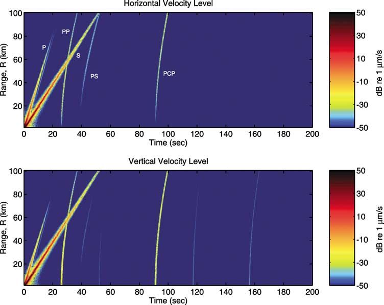
148                                                     S. Lee et al. / Icarus 165 (2003) 144–167

Fig. 4. The radiated seismo-acoustic energy spectrum (f ) defined by           Fig. 5. The radiated energy level L from surface cracks for various crack
Eqs. (C.9) and (C.41) as a function of crack depth h. The amplitude of          depths h, as defined in Eq. (C.42).
the spectrum is proportional to h6 , and the peak frequency and bandwidth
are inversely proportional to h.

that the choice of Young’s modulus does not change the rel-
ative energy levels between the cracks of various depths, and
the signal-to-noise ratio analysis in this paper remains valid.
   The crack is also assumed to open as a linear function of
time over a period equal to the maximum crack width over
the crack propagation speed, as shown in Fig. C.1. The crack
propagation speed is taken to be
v  0.9cs ,                                                          (4)
following standard models of fracture mechanics (Aki and
Richards, 1980) and experimental measurements of cracks
on ice at terrestrial temperatures (Lange and Ahrens, 1983;
Stewart and Ahrens, 1999). The opening time of the crack is
then directly proportional to the crack depth h.
   The source energy spectrum for a general crack of depth                      Fig. 6. The radiated energy level L for various radii rm of impactors, as
h is given in Fig. 4, from which it can be seen that the                        defined in Eq. (C.56). Solid lines represent energy levels of rock impactors
frequency of the peak and 3-dB bandwidth are inversely pro-                     with density ρ = 3 g/cm3 and impact velocity v = 20 km/s. Energy levels
portional to crack depth h while the peak energy spectral                       of iron meteors with ρ = 7 g/cm3 and v = 30 km/s, and those of comets
density grows with a dramatic h6 proportionality. This is il-                   with ρ = 1 g/cm3 and v = 8 km/s are also shown as errorbars in the figure.
lustrated in Fig. 5, where source energy spectral levels are
given for various crack depths and it is clear that Big Bang                    the entire satellite (Bierhaus et al., 2001; personal communi-
events, with depths exceeding 150-m depths, will be at least                    cation with E.B. Bierhaus). To determine the source energy
36 times more energetic than the nominal 50-m deep cracks                       spectrum for impacts as a function of impactor size, com-
expected solely from diurnal tides.                                             position and speed, we make use of the impact-explosion
   From Eq. (3), the opening widths of the cracks will be                       analogy discussed in Melosh (1989). A derivation of the
0.3 mm and 8 mm for 50-m and 250-m cracks, respectively.                        radiated energy spectrum using underground explosion phe-
Such small-scale surface motions and feature changes will                       nomenology is given in Appendix C.2.
not be readily observable from orbit, but could easily be de-                      The radiated energy spectral levels for impactors of var-
tected by seismo-acoustic sensors.                                              ious radii are shown in Fig. 6, assuming a nominal rock
                                                                                meteor with 3 g/cm3 density and 20 km/s impact velocity.
3.2. Impacts                                                                    This energy level will vary within ±10 dB depending on the
                                                                                seismic efficiency discussed in Appendix C.2.
   The rate of small impacts on Europa, for impactors in the                       Small impacts, then may provide another source of Big
1–10-m radius range, is poorly constrained. A recent model                      Bang events that have energies well above those expected
predicts a rate of 0.2 to 16 for such impacts per year over                     solely from tensile cracks driven by diurnal tides and may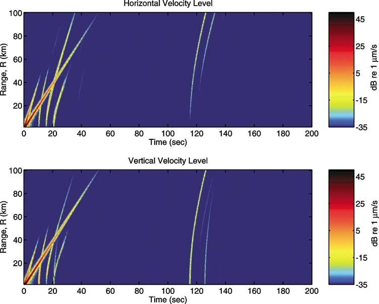
Probing Europa’s interior with natural sound sources                                               149

be frequent enough to be used as sources of opportunity for                    where J0 is the Bessel function of the first kind, kr is the
echo-sounding.                                                                 horizontal wavenumber, and

                                                                               kz,m = km  2 − k2,
                                                                                               r                                       (13)
4. Seismo-acoustic wave propagation on Europa
                                                                               κz,m = κm  2 − k2,
                                                                                               r                                       (14)
    The radiated field from tensile cracks typically have di-
                                                                               are the vertical wavenumbers.
rectionality, but here we assume that an omnidirectional
                                                                                  The inhomogeneous Helmholtz equation with a mono-
source, or a monopole, should best describe the expected or
                                                                               pole source at r = 0, z = z ,
average directionality.
    Assuming a time-harmonic acoustic field at frequency f ,
                                                                                       2                          δ(r)
the equation of motion in horizontally stratified, homoge-                      ∇ 2 + km  Gφ,m (r, z, z , f ) = −      δ(z − z )                  (15)
                                                                                                                   2πr
neous, isotropic elastic media can be expressed in cylindrical                 has solution in the form of the integral representation
coordinates (r, z) as (Schmidt and Tango, 1986)
                                                                                                            ∞
                                 ∂
                                                                               φ,m (r, z, z , f ) = − 1         eikz,m |z−z |
u̇m (r, z, f ) = −i2πf S(f )        Gφ,m (r, z, f )                            G                                                J0 (kr r)kr dkr .   (16)
                                 ∂r                                                                    4π            ikz,m
                                                                                                            0
                                      ∂2
                                 +        Gψ,m (r, z, f )                      The inhomogeneous solution for SV component G       ψ,m is
                                    ∂r∂z
               ≡ S(f )Gu̇,m (r, z, f ),                       (5)              zero, since an omnidirectional source does not excite SV
                                                                              component.
                                  ∂
ẇm (r, z, f ) = −i2πf S(f )         Gφ,m (r, z, f )                              Two-dimensional simulations including radial and verti-
                                 ∂z                                            cal components are sufficient since out-of-plane motion does

                                    1 ∂ ∂                                      not occur for the assumed monopole source. A stable nu-
                                 −       r Gψ,m (r, z, f )
                                    r ∂r ∂r                                    merical solution in the frequency domain is obtained by
               ≡ S(f )Gẇ,m (r, z, f ),                       (6)              wavenumber integration (Schmidt and Tango, 1986; Kim,
                                                                               1989). The time domain solution and synthetic seismograms
where {u̇m , ẇm } are the radial and vertical velocity com-
                                                                               are then obtained by Fourier synthesis.
ponents, {Gφ,m , Gψ,m } are solutions to compressional (P)
                                                                                  In this section, we investigate wave propagation in Eu-
and shear vertical (SV) displacement potential Helmholtz
                                                                               ropa through transmission loss, time-range, and synthetic
equations in each layer m with corresponding compressional
                                                                               seismogram analysis.
wave speed cp,m and shear wave speed cs,m , and S(f ) is the
spectral amplitude of volume injection by the source at fre-
                                                                               4.1. Transmission loss
quency f .
   The solutions are composed of the homogeneous and in-
                                                                                  Transmission loss is a measure of the acoustic field level
homogeneous solutions of the Helmholtz equations,
                                                                               as a function of position, and is calculated in the frequency
       φ,m + G
Gφ,m = G      φ,m ,                                                (7)        domain for a time-harmonic source via
       ψ,m + G
Gψ,m = G      ψ,m .                                                (8)                                  |u̇(r, r )|
                                                                               TLu̇ (r, r ) = −20 log10               dB re rref ,
The homogeneous solutions satisfy                                                                         |v̇0 (r )|
 2
       2                                                                                                 |ẇ(r, r )|
 ∇ + km  Gφ,m (r, z, f ) = 0,                                       (9)        TLẇ (r, r ) = −20 log10                dB re rref ,                (17)
 2                                                                                                       |v̇0 (r )|
       2
 ∇ + κm Gψ,m (r, z, f ) = 0,                                       (10)
                                                                               where u̇(r, r ) and ẇ(r, r ) are the horizontal and vertical ve-
where km = 2πf/cp,m and κm = 2πf/cs,m are wavenum-                             locity fields at point r for a source at point r , and v̇0 (r ) is
bers of compressional and shear waves. The homogeneous                         the velocity produced at a distance of rref = 1 m from the
solutions can be expressed in the wavenumber domain using                      same source in an infinite, homogeneous medium with den-
integral representations,                                                      sity ρ(r ) and compressional wave speed cp (r ).
                    ∞                                                             The magnitudes of the vertical and horizontal particle

φ,m (r, z, f ) =
G                         A−
                           me
                              −ikz,m z
                                       + A+
                                          me
                                             ikz,m z                           velocities of an ice source 50-m below the ice-vacuum in-
                                                                               terface in the 20-km convecting ice shell model are shown
                    0
                                                                               in Fig. 7 at 2-Hz frequency, corresponding to the central
                  × J0 (kr r)kr dkr ,                              (11)
                                                                               frequency typical in a Big Bang source event. This fig-
                  ∞
                     − −iκ z                                                 ure shows the transmission and reflection of acoustic waves

Gψ,m (r, z, f ) =    Bm e z,m + Bm    + iκz,m z
                                       e                                       from the ice–water and water–mantle interfaces at up to 200-
                    0                                                          km range. Fringes in the source radiation pattern due to the
                    × J0 (kr r) dkr ,                              (12)        free surface boundary condition at the ice-vacuum interface
150 S. Lee et al. / Icarus 165 (2003) 144–167
are visible as are modal interference patterns in the ice layer. at a receiver simultaneously since their ray paths are sym-
These patterns are a function of frequency, and are not read- metric. Also, an S wave from a source to a receiver on the
ily observable for a typical broadband ice-crack or impact ice-vacuum surface is a Rayleigh wave.
source. As expected, the horizontal particle velocity field in Some labelled ray geometries are shown in Fig. 8. A ray
the ocean directly beneath the source is very weak due to path follows a straight line in an iso-speed medium. How-
the almost total reflection of the shear wave at the ice–water ever, if the sound speed in the medium varies along the ray
interface, which cannot support horizontal shear. path, the ray must satisfy Snell’s law where reflection and
Figure 7 illustrates how efficiently seismic waves propa- transmission will occur at the boundary between iso-speed
gate through the ice shell as do acoustic waves through the layers, and a continuous bending of a ray path, or refrac-
subsurface ocean, and how a geophone located at the top of tion, will occur given a continuous sound speed gradient. For
the ice shell will be able to detect multiple reflections from a horizontally stratified medium where sound speed varies
the ice–water interface as well as the water–mantle interface. only in the z-direction, the radius of curvature rc of a re-
The Rayleigh wave is a surface wave that travels at fracting ray is
roughly 90% of the medium shear speed for a homogeneous
c0 dc −1
halfspace, and suffers only cylindrical spreading in horizon- rc = , (18)
tal range but is attenuated exponentially with depth from sin θ0 dz
the surface it travels on. It will be strongly excited on the where θ0 is the incident angle at some fixed depth as in Fig. 8
ice-vacuum interface by sources of shallow depth, such as and c0 is the sound speed at the same depth. For the 20-km
surface cracking events, impacts and the near-surface source convective ice shell model, the minimum radius of curvature
of the given example. It can be seen in Fig. 7 as a strong ver- of a compressional wave in upper thermal boundary layer
tical velocity field trapped near the surface. Characteristic regime is 51 km, which is not perceptible in Fig. 7. Re-
differences between the Rayleigh wave and direct compres- fracted propagation of sound is a common feature in terres-
sional wave arrivals will prove to be useful in determining trial oceans. In mid-latitudes deep sound channels typically
the range of surface sources of opportunity. The frequency- form due to thermal heating above and increasing pressure
dependent characteristics of a Rayleigh wave may also be below. These enable sound waves to propagate for thousands
used as another possible tool to probe the interior structure of kilometers without ever interacting with the sea surface or
of the ice shell, and will be described in Section 7.2. If the bottom (Urick, 1983). Without more evidence, however, it is
wavelength of the Rayleigh wave is long compared to the difficult to speculate on what sound speed profiles may exist
thickness of the ice shell, it will propagate as a flexural wave in a potential Europan ocean.
on a thin plate. The travel time from a source to receiver depends on the
ray path. Travel time differences between ray paths can be
4.2. Nomenclature of acoustic rays used to infer Europa’s interior structure. The range between
a surface source event and a surface geophone can be ob-
The analysis of seismo-acoustic wave propagation from tained from direct P and S wave arrivals given the compres-
a source to receiver can be intuitively understood by apply- sional and shear wave speeds in ice, which can be estimated
ing ray theory which is valid when the wavelength is small with reasonable accuracy based on a priori information (see
compared to variations in the medium. Rays are defined as Appendix A). With the additional travel time measurement
a family of curves that are perpendicular to the wavefronts of a single ice–water reflection, such as PP, PS, or SS, the
emanating from the source, and are obtained by solving the
eikonal equation (Brekhovskikh and Lysanov, 1982; Frisk,
1994; Medwin and Clay, 1998).
In order to describe the various seismo-acoustic rays
propagating in ice and water layers, a nomenclature is
adopted where P represents a compressional wave in the
ice shell, S a shear wave in the ice shell, and where C is an
acoustic wave in the subsurface ocean that includes reflec-
tion from water–mantle interface. Following this convention,
appropriate letters are added consecutively when an acoustic
ray reflects from or transmits through a given environmental
interface. A PS wave, for example, is a compressional wave
that departs from the source, reflects as a shear wave at the
ice–water interface and arrives at the receiver. A PCS wave
Fig. 8. Nomenclature of acoustic rays. PP, PS, SS waves are single re-
is a compressional wave that transmits through the ice–water flections from the ice–water interface, and PPPP, SSSS waves are double
interface, reflects from the water–mantle interface, returns to reflections from the ice–water interface. PCP, PCS, and SCS waves are the
the bottom of the ice shell, and transmits back into the ice as reflections from the water–mantle interface. Sound speeds in ice layer and
a shear wave. It should be noted that SP and PS waves arrive ocean layer are assumed constant in this figure.Probing Europa’s interior with natural sound sources 151
thickness of the ice shell can be estimated. If more than one Inspection of the various scenarios indicates that the over-
of these reflected paths are used, the sound speed in ice can all pattern of arrivals and amplitudes is very sensitive to the
also be experimentally estimated to improve upon the a pri- structure of Europa’s ice–water layer, in particular, the ab-
ori information. Once the range of the source and the ice solute thicknesses and depths of the ice shell and ocean, as
shell thickness are obtained, the depth of a subsurface ocean expected from basic echo-sounding principles. The pattern,
can be estimated by the reflections from the water–mantle however, is not very sensitive to the differences in internal
interface, using any of the PCP, PCS, or SCS ray paths. The temperature of the rigid versus convecting ice models, as can
use of this kind of travel time analysis to infer Europa’s in- be seen by comparing Figs. 9 and 12. Other techniques in-
terior structure will be discussed in more detail in Section 5. volving seismo-acoustic tomography may be better suited to
estimating the temperature structure.
4.3. Synthetic seismograms for a Big Bang event Detailed characteristics of the time series measured by a
surface geophone can be better observed in synthetic seis-
mograms. We present illustrative examples for the 20-km
Here we study the amplitude and arrival-time structure of
convective ice shell model. Figures 13 and 14 present a sce-
a Big Bang surface source event as measured by a triaxial
nario where the seismometer is located at short range (2-km)
geophone on Europa’s surface for the four stratified models
from the source, while Figs. 15 and 16 present a longer range
of Europa described in Section 2. First we consider the ar-
(50-km) scenario. In both scenarios, a sufficiently diverse set
rival time and amplitude structure as a function of range be- of prominent and well separated arrivals are found to enable
tween the surface source and receiver by identifying the di- the source range, as well as the thickness of Europa’s ice
rect arrivals and reflections from various internal strata. Then shell and ocean layer to be determined by echo sounding.
we look in more detail at the type of amplitude and arrival For the case of a short source-receiver separation, as in
time measurements that may be made at specific ranges. The Fig. 13, both the direct P and S waves arrive so near in time
analysis proceeds by solving the full-field seismo-acoustic that they cannot be distinguished. The P wave is in fact over-
wave equations of Eqs. (5) to (16) for a Big Bang source whelmed by the S wave, which is effectively the Rayleigh
with a spectral peak in the 1–4-Hz range. The source is here wave due to the proximity of the source and receiver to
modeled as a monopole at 50-m depth and the receiver as a the free surface. All subsequent arrivals can be easily dis-
triaxial geophone at 1-m depth beneath the ice-vacuum sur- tinguished from each other since they are well separated
face. The finite bandwidth of the radiation is computed by in time. The first arrivals are multiple reflections from the
Fourier synthesis. The resulting simulations are referred to ice–water interface. For such a short source-receiver separa-
as synthetic seismograms when they show amplitude ver- tion, waves returning from the water arrive at near normal
sus time, and time-range plots when they show amplitude incidence to the ice–water interface in the present geome-
versus time and range. All simulations in this section have try, and so lead to very weak SV transmission into the ice.
been performed for h = 250-m cracks or equivalently an im- This explains the relative abundance of prominent and well
pactor of roughly 10-m radius. These figures can be scaled separated arrivals from the mantle in vertical velocity and
for various crack depths h and impactor volume injections s0 the paucity of such arrivals in horizontal velocity at the geo-
using Figs. 5 and 6, as explained in Appendix C (Eqs. (C.30) phone in Fig. 14.
to (C.33)). For the case of a much longer source-receiver separation,
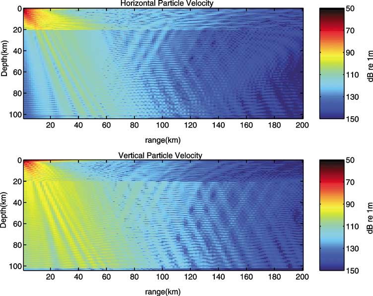
Time-range plots are shown in Figs. 9 and 10 for the con- as in Fig. 15, the direct P and S (again, the Rayleigh wave),
vective ice shell model, and Figs. 11 and 12 for the rigid as well as multiple reflections from ice–water and water–
ice shell model. In each figure, two lines consistently de- mantle interfaces are well separated in the time domain.
part without curvature from the origin. These are the direct
P wave and Rayleigh wave arrivals in the ice. The Rayleigh
wave has the highest amplitude since it propagates as a 5. Inferring Europa’s interior structure by travel time
trapped wave on the ice-vacuum surface. analysis
Arrivals due to multiply reflected paths from the ice–
water interface and the water–mantle interface are also read- 5.1. Simplified Europa model
ily observed. The travel time differences between the mul-
tiple reflections are closely related to the thickness of the In the previous section, we showed that the arrival time
ice shell. In the thin ice shell model (Fig. 11), the spacing structure of seismo-acoustic waves is far more sensitive to
between the multiple reflections is not much greater than ice shell thickness and ocean depth than to the temperature
the duration of the source event. This leads to one group of variations in the ice shell associated with the various rigid
closely spaced arrivals reflected from the ice–water interface and convecting models examined. The seismo-acoustic pa-
and another closely spaced group from the water–mantle in- rameters most important to the measured arrival-time struc-
terface. As the thickness of the ice shell increases, these ture, namely the thickness of the ice shell and the depth
multiple reflections separate more in the time domain as can of a subsurface ocean, can then be estimated by matching
be seen in Figs. 9, 10, and 12. measured travel times with those derived from a simplified152
S. Lee et al. / Icarus 165 (2003) 144–167
Fig. 7. Transmission loss plots of the horizontal particle velocity TLu̇ (top) and vertical particle Fig. 9. Time-range plot for the 20-km convective ice shell model. Colors represent the horizontal
velocity TLẇ (bottom) as defined in Eq. (17), when the source is located 50-m below the surface. velocity level Lu̇ (top) and vertical velocity level Lẇ (bottom), as defined in Eqs. (C.18) and (C.19).
Fig. 10. Time-range plot for the 50-km convective ice shell model. Fig. 11. Time-range plot for the 5-km rigid ice shell model.Probing Europa’s interior with natural sound sources 153
Fig. 20. Time-range plot for a Big Bang event that can stand above the reference ambient noise
level of −35 dB re 1 µm/s.
Fig. 13. Ice-water reflections at 2-km range for the 20-km convective ice
shell model. The top figure shows the horizontal velocity level Lu̇ and the
bottom figure shows the vertical velocity level Lẇ , as defined in Eqs. (C.18)
and (C.19). The regular spacing between the reflections can be directly re-
lated to the thickness of the ice shell. Direct P wave and Rayleigh wave
arrivals are not well separated for this short range propagation.
Europan model. The simplified model drops parameters of
Fig. 2 that do not have a first order effect in the arrival time
Fig. 12. Time-range plot for the 20-km rigid ice shell model.
structure. This leaves the six parameters shown in Fig. 17 at
the top of the hierarchy. Dropped parameters, low in the hi-
erarchy for the present echo-sounding technique, may be far
more important in other inversion schemes.
The simplified Europa model employs an iso-speed ice
shell. This is justified to first order for a number of reasons.
Although Europa’s ice layer may undergo a drastic change
in temperature with depth, from roughly 100 to 273 K, the
corresponding variations of cp and cs do not exceed 5%, as
shown in Appendix A, except where the temperature reaches
a few degrees of the melting point. This, however, occurs
only over a small portion of the lower thermal boundary in
the ice shell, as shown in Fig. 1. While the ice in this region
undergoes changes in its molecular behavior, the change in
sound speed is less than 10%. The overall error associated
with the iso-speed assumption will then be less than 10%.
In the simplified Europa model, we may further assume that
ξ ≡ cp /cs = 2, which is a typical value for ice (Fig. A.1(c)).
5.2. General nondimensionalized travel time curves
Under the assumption of an iso-speed ice shell, following
the simplified Europan model, the general surface source-154 S. Lee et al. / Icarus 165 (2003) 144–167
Fig. 14. Bottom reflections at 2-km range for the 20-km convective ice shell Fig. 15. Ice-water reflections at 50-km range for the 20-km convective ice
model. The bottom reflections for short range propagation are mostly com- shell model. Travel time differences between the direct P wave and the
pressional wave reflections, and are more prominent in the vertical particle Rayleigh wave can be inverted for the range between the source and re-
velocity components. The weak precursor before the PCP reflection is the ceiver, and multiple reflections from the ice–water interface can be inverted
reflection from the sediment layer overlying the basalt halfspace. for the thickness of the ice shell.
to-receiver travel time of ice–water reflected paths can be
determined as a function of two nondimensional parameters Rayleigh wave. The Rayleigh wave can be easily identified
ξ and R/H , as shown in Appendix B. The travel time curves by its high amplitude and retrograde particle motion where
become functions of only one nondimensional parameter vertical and horizontal components are 90◦ out of phase.
R/H , if we assume the typical value ξ = 2. Nondimensional To also estimate the thickness of the ice shell, at least one
travel time curves for the simplified Europa model are plot- reflection from the ice–water interface must also be identi-
ted in Fig. 18 where the travel time for paths including up to fied. The PP wave arrival can be readily identified since it
double reflections from the ice–water interface are shown. arrives the soonest after the direct P wave except when R/H
This figure can be used to analyze arrivals from ice–water is less than one, as shown in Fig. 18. Even in this case, how-
reflections in Figs. 9 to 12. ever, the PP wave can be easily identified, since, besides the
Similarly, the general source-to-receiver travel time of direct P wave, the Rayleigh wave is the only wave that can
paths involving water–mantle reflections can also be deter- arrive before it.
mined in terms of the additional nondimensional parame- If, for example, we measure the travel time differences
ters ξw ≡ cp /cw , the ratio between the compressional wave ts − tp ≡ ∆s , and tpp − tp ≡ ∆pp , where tp , ts , and tpp are
speed in ice and water, and Hw /H , the ratio between the the travel times of the direct P, the Rayleigh, and PP waves,
ocean depth and the ice shell thickness, assuming an iso-
speed water column. This is also shown in Appendix B. 1 1 1 ξ
Nondimensional travel time curves for these paths are also ∆s = − R= − 1 R, (19)
plotted in Fig. 18, assuming Hw /H = 4 and ξw = 4/1.5. 0.93 cs cp cp 0.93
1
5.3. Estimating interior structure ∆pp = 4H 2 + R 2 − R , (20)
cp
The range between the source and receiver can be deter- and R/cp and H /cp are uniquely determined by,
mined with a single triaxial geophone on Europa’s surface
without knowledge of the ice thickness by measuring the R ∆s
travel time difference between the direct P wave and the = , (21)
cp ξ/0.93 − 1Probing Europa’s interior with natural sound sources 155
Fig. 17. Schematic diagram of the simplified Europa model used for the
parameter inversion. R is the range between the source and seismometer.
The ice shell and ocean are simplified into iso-speed layers.
sional and shear speed in ice is known, the error in the range
and thickness estimates will be linearly related to the error in
Fig. 16. Bottom reflections at 50-km range for the 20-km convective ice compressional wave speed. Based on the analysis presented
shell model. For long range propagation, bottom reflections are prominent in Appendix A, the sound speed in ice can be estimated to
in both the horizontal and vertical particle velocity components.
within roughly 10%. The range of the source and the thick-
ness of the ice shell can then also be estimated within 10%
and of error given the travel times of the direct P, the Rayleigh,
1/2 and PP waves. Estimates of R, H , cp , and cs can be refined
H 1 2∆s
= ∆pp ∆pp + . (22) by analyzing arrivals from other paths. Similarly, the ocean
cp 2 ξ/0.93 − 1
thickness Hw and average sound speed cw can be determined
This result shows that if the compressional wave speed by using Fig. 18 to analyze arrivals from paths reflecting
in the ice is uncertain, but the ratio between the compres- from the water–mantle interface.
Fig. 18. Nondimensionalized travel time curves for direct paths, ice–water reflections, and water–mantle reflections. It is assumed that Hw /H = 4 and
ξw = 4/1.5 for bottom reflections. This figure can be directly compared to Figs. 9 and 12.156 S. Lee et al. / Icarus 165 (2003) 144–167
6. Europan ambient noise spanned by the geophone and so is smaller by a factor of 2.
The ambient noise levels in decibels are defined by
As noted in the introduction and in Section 3.1, there is
|Nu̇ |2
a possibility that ice cracking events on Europa may occur NLu̇ = 10 log dB re u̇ref , (26)
so frequently in space and time that their accumulated ef- u̇2ref
fect may lead to difficulties for the proposed echo-sounding |Nẇ |2
technique. Here we attempt to quantify the characteristics NLẇ = 10 log 2
dB re ẇref , (27)
ẇref
of a Big Bang event necessary for it to serve as a source of
opportunity in echo sounding given an estimate of the accu- where u̇ref = ẇref = 1 µm/s.
Equations (23) and (24) are used to compute the gen-
mulated noise received at a surface geophone. We do so by
eral ambient noise levels measured by a geophone at 1-m
first developing a Europan noise model in terms of the spatial
below the ice-vacuum interface for the 20-km convective
and temporal frequency and source spectra of the expected
shell model as a function of temporal and spatial source den-
noise sources.
sity. The results are shown in Fig. 19 for noise sources at
z = 50-m depth in the 1–4-Hz band, the same depth and
6.1. Estimation of ambient noise level
band used for the Big Bang synthetic seismograms of Sec-
tion 3. This noise table is for h = 50-m ambient cracks, but
In order to calculate the ambient noise level, an ocean
can be scaled for other crack depths h by following the pro-
acoustic noise modeling technique (Kuperman and Ingenito,
cedures described in Appendix C.
1980) is adapted for Europa. The basic assumption is that
The ambient noise levels of Fig. 19 can be compared di-
the noise arises from an infinite sheet of monopole sources rectly with the signal levels of 250-m cracks for the 20-km
just below Europa’s ice-vacuum boundary at depth z . The convective shell model (Figs. 9, 13, 14, 15, and 16). The
sources are assumed to be spatially and temporally uncor- noise levels can even be compared with the signal levels in
related and to have the same expected source cross-spectral Figs. 10, 11, and 12 because ambient noise level does not
densities. vary significantly as a function of ice shell thickness, since
The mean-square horizontal and vertical particle veloci- it is dominated by the Rayleigh wave, which is trapped on
ties of the ambient noise measured by a geophone at depth z the ice-vacuum interface and so is relatively insensitive to
resulting from these uncorrelated sources are respectively the ice shell thickness H when its wavelength is small com-
∞ pared to H .
π 2 Such comparisons still require knowledge of the spatial
|Nu̇ | =
2
S(f )
(0T )(0A) and temporal densities of the noise sources. These can be
−∞
estimated for diurnal tidally driven tensile cracks by not-
∞ ing that a cycloidal feature will extend at a speed of roughly
gu̇ (kr , z, z ) kr dkr df,
2
× (23) 3.5 km/hr, following the location of maximum tensile stress
0
∞
2π 2
|Nẇ | =
2
S(f )
(0T )(0A)
−∞
∞
gẇ (kr , z, z ) kr dkr df,
2
× (24)
0
where 1/0T and 1/0A are temporal and spatial densi-
ties of noise sources, |S(f )|2 is the expectation of the
magnitude squared of source spectrum of a given source,
and gu̇ (kr , z, z ) and gẇ (kr , z, z ) are the integral representa-
tions of the horizontal and vertical particle velocities in the
wavenumber domain, which are defined in terms of Hankel
transform of Eqs. (5) and (6),
∞
gu̇,ẇ (kr , z, z ) = Gu̇,ẇ (r, z, z )J0 (kr r)r dr. (25)
0 Fig. 19. Ambient noise levels in the horizontal velocity NLu̇ and vertical
velocity NLẇ , as defined in Eqs. (23) and (24), for the 20-km convective ice
The variance of the vertical particle velocity is the same as shell model as a function of spatial densities and temporal emission rates of
the scalar result given in Wilson and Makris (2003). The hor- the surface cracks. The reference ambient noise levels assuming 0T = 60 s
izontal component is for one out of two horizontal directions and 0A = 100 km2 are marked in the figure.Probing Europa’s interior with natural sound sources 157
(Hoppa et al., 1999). The propagation speed of a tensile tures that occur at a rate inversely proportional to the maxi-
crack, however, is the much larger v 0.9cs , as noted in mum depth of the crack h. Larger cracks will be less frequent
Section 3.1. The cycloidal features then are apparently com- and so less likely radiate seismo-acoustic waves that overlap.
prised by a sequence of discrete and temporally disjoint Larger cracks will also release stress over larger areas and so
cracking events. If we assume that each tidally driven crack, prevent other cracks from developing nearby.
of nominal depth h = 50-m extends for a minimum length Small impacts are another potential source of Big Bang
of h = 50-m, as discussed in Section 3.1, we arrive at a events that usually have much higher energy spectral levels
rate of roughly 1 tensile crack per minute along a given than surface cracks, as can be seen by comparing Figs. 5
cycloidal feature. A consistent estimate of the spatial separa- and 6. Given the impact rate mentioned in Section 3.2, the
tion between cracking events would be the roughly 100-km probability of at least one impactor within 100 km of the
scale of a cycloidal feature (Hoppa et al., 1999). As can seismometer is 0.1 to 10% assuming a 4 month operational
be observed in Fig. 19, the ambient noise level reaches period. While such an impact is not highly likely, the signal-
−35 dB re 1 µm/s for 100-km crack spacing and 1 discrete to-noise ratio would be large and the reflections could be
emission per minute. easily resolved. Smaller impacts may be much more frequent
If the source of opportunity and ambient noise sources and still energetic enough to serve as Big Bang events, but
have the same depth of h = 50-m, the expected energy of their rates are difficult to resolve with current observational
each noise source equals that of the signal. In this case, methods.
the amplitudes of the time-range plots and synthetic seismo- Our signal-to-noise-ratio analysis is based on the worst-
grams in Section 4.3 should be decreased by 56-dB, as can case scenario of maximum diurnal stress, where all sur-
be determined from Eqs. (C.30) and (C.31) of Appendix C. face cracks are assumed to actively radiate seismo-acoustic
Comparison with the time-range plots and synthetic seismo- waves once every minute. Cracking will become less fre-
grams of Section 4.3, after subtracting 56-dB to go from an quent after Europa passes the perigee. The ambient noise
h = 250-m to an h = 50-m deep crack, shows that the reflec- level will then decrease, enabling echo-sounding with a sur-
tions from the ice–water and water–mantle interfaces will be face crack of shallower depth h. Since impactors are totally
buried by the ambient noise for this scenario. The situation independent of surface cracking noise, they may strike Eu-
changes if the source of opportunity is far more energetic ropa at low-tide when surface cracks are dormant, achieving
than an expected noise event, as is the case for a Big Bang the maximum signal to noise ratio.
source event.
6.2. Estimation of signal to noise ratio
7. Inferring interior properties of Europa with love and
It was shown in Section 3.1 that the peak of the energy Rayleigh waves
spectral density for a surface crack is proportional to h6 ,
while both the bandwidth and frequency of the spectral peak Love waves are effectively propagating SH modes trapped
are inversely proportional to the crack depth h. Smaller by the boundaries of an elastic waveguide, while Rayleigh
cracks will then not only radiate less energy, they will also waves are interface waves that travel along an elastic surface
spread this energy over a broader and higher frequency spec- that involve both compressional and SV wave potentials.
trum. Larger cracks, on the other hand, will radiate more en- The theory of these waves in horizontally stratified media is
ergy over smaller bandwidths at lower frequencies, as shown well developed (see, e.g., Brekhovskikh, 1980; Miklowitz,
in Fig. 4. This would make it advisable to low-pass filter geo- 1978). Here we discuss the possibility of using the frequency
phone time series data to the band of a Big Bang source of dependent characteristics of these waves to infer interior
opportunity, if this source was due to a much deeper and properties of Europa.
less frequent cracking event than those comprising the ex-
pected noise. If the Big Bang is 5 times deeper than the
7.1. Dispersion of the Love wave
ambient cracks, for example, the radiated energy within the
bandwidth of the Big Bang will be approximately 56-dB
greater than that radiated by an ambient crack. This will If an elastic medium is surrounded by a vacuum or fluid
in turn increase the signal-to-noise ratio of the time series media that does not support shear, as in the case of an ice
by 56-dB. In this case, it will be possible to robustly detect sheet floating on an ocean, the Love wave will propagate
multiple Big Bang reflections from the ice–water interface like a free wave in a plate.
and water–mantle interface above the noise for nominal 50- Considering the geometry in Fig. 21, it can be shown that
m deep noise cracks of 100-km spacing and 1 per minute SH waves will propagate as discrete normal modes with the
rate, as is illustrated in Fig. 20 for a 250-m deep Big Bang group velocity of each mode given as
crack.
2 1/2
According to Nur (1982), unfractured ice subject to a πl
fixed tensile stress will develop a distribution of surface frac- Ul = c s 1 − , l = 0, 1, . . . , lmax . (28)
κH158 S. Lee et al. / Icarus 165 (2003) 144–167
The maximum number of normal modes for a given fre- group velocity and cut-off frequency of each mode is given
quency is by
κH 2 − κ2
lmax = integer part of , (29) H κx,l b µb
2 − κ2
κx,l b
π Ul = κx,l + 1+
cos2 (H κ 2 − κ 2 ) µ κ2 − κ2
with the cut-off frequency of each mode is given as x,l x,l
cs l H 2 − κ2
κx,l
fc,l = . (30) κ b
2H ×
cs cos2 (H κ 2 − κ 2 )
It is important to note that there is a zeroth-order mode x,l
that is non-dispersive, insensitive to the thickness, and has no −1
κ κx,l − κb
2 2
cut-off frequency, which can be obtained by setting l = 0 in µb κ b
+ + , (31)
Eqs. (28) and (30). This characteristic of zeroth-order mode µ csb cs κ 2 − κ 2
x,l
is also shown in Fig. 22.
This derivation shows that Love waves in a free or fluid l cs csb
fc,l = , (32)
loaded plate have group velocities that are inversely propor- 2H c2 − c2
sb s
tional to frequency so that the lower frequency components
propagate slower than the higher ones. This dispersive char- where κx,l is the wavenumber of lth mode in x direction,
acteristic is shown for the group velocity of the 1st mode for and µb , csb , κb are the shear modulus, shear wave speed, and
various ice shell thicknesses in Fig. 22. shear wavenumber in the elastic medium underlying the ice
If the ice shell overlies another elastic medium with faster shell, respectively. The mode shapes and dispersion curves
shear wave speed such as Europa’s mantle, however, at the for various ice shell thicknesses assuming an ice shell over-
low frequency end the dispersion relationship will be re- lying basalt halfspace are shown in Figs. 23 and 24, respec-
versed with the lower frequency components arriving faster tively.
than the higher frequency components. This is a common Kovach and Chyba (2001) have argued that it may be pos-
effect also observed in ocean acoustic waveguides (Pekeris, sible to verify the existence of a subsurface ocean on Europa
1948; Frisk, 1994). In this case, it can be shown that the by finding a way to measure the presence or absence of this
reversal. Since the Love wave is trapped within the ice shell,
Fig. 21. Love wave geometry and mode shapes for an elastic plate sur-
rounded by fluid media.
Fig. 23. Love wave geometry and mode shapes assuming an ice shell over-
lying basalt halfspace.
Fig. 22. Love wave dispersion curves for various ice shell thicknesses as-
suming an iso-speed ice shell with a shear wave speed cs = 2 km/s, over-
lying a subsurface ocean. The 0th order mode has a constant group velocity Fig. 24. Love wave dispersion curves for the 0th and 1st order modes in the
that is independent of the ice shell thickness. case where ice shell is overlying a basalt halfspace.You can also read