THE ROLAND VON GLASOW AIR-SEA-ICE CHAMBER (RVG-ASIC): AN EXPERIMENTAL FACILITY FOR STUDYING OCEAN-SEA-ICE-ATMOSPHERE INTERACTIONS
←
→
Page content transcription
If your browser does not render page correctly, please read the page content below
Atmos. Meas. Tech., 14, 1833–1849, 2021
https://doi.org/10.5194/amt-14-1833-2021
© Author(s) 2021. This work is distributed under
the Creative Commons Attribution 4.0 License.

The Roland von Glasow Air-Sea-Ice Chamber (RvG-ASIC):
an experimental facility for studying ocean–sea-ice–atmosphere
interactions
Max Thomas1,2 , James France1,3,4 , Odile Crabeck1,5,6 , Benjamin Hall7 , Verena Hof8 , Dirk Notz8,9 , Tokoloho Rampai7 ,
Leif Riemenschneider8 , Oliver John Tooth1 , Mathilde Tranter1 , and Jan Kaiser1
1 Centre  for Ocean and Atmospheric Sciences, School of Environmental Sciences, University of East Anglia,
NR4 7TJ, Norwich, UK
2 Department of Physics, University of Otago, P.O. Box 56, Dunedin 9054, New Zealand
3 British Antarctic Survey, Natural Environment Research Council, Cambridge CB3 0ET, UK
4 Department of Earth Sciences, Royal Holloway, University of London, Egham TW20 0EX, UK
5 Laboratoire de Glaciologie, Université Libre de Bruxelles, Bruxelles, Belgium
6 Unité d’Océanographie Chimique, Freshwater and Oceanic sCience Unit reSearch (FOCUS),

Université de Liége, Liége, Belgium
7 Chemical Engineering Department, University of Cape Town, Cape Town, South Africa
8 Max Planck Institute for Meteorology, Hamburg, Germany
9 Center for Earth System Research and Sustainability (CEN), University of Hamburg, Hamburg, Germany

Correspondence: Jan Kaiser (j.kaiser@uea.ac.uk)

Received: 29 September 2020 – Discussion started: 14 October 2020
Revised: 6 January 2021 – Accepted: 27 January 2021 – Published: 5 March 2021

Abstract. Sea ice is difficult, expensive, and potentially dan-    centre of the tank but drops to as low as 60 % of the max-
gerous to observe in nature. The remoteness of the Arctic          imum intensity in one corner. The temperature sensitivity
Ocean and Southern Ocean complicates sampling logistics,           of our light sources over the 400 to 700 nm range (PAR)
while the heterogeneous nature of sea ice and rapidly chang-       is (0.028 ± 0.003) W m−2 ◦ C−1 , with a maximum irradiance
ing environmental conditions present challenges for con-           of 26.4 W m−2 at 0 ◦ C; over the 320 to 380 nm range, it
ducting process studies. Here, we describe the Roland von          is (0.16 ± 0.1) W m−2 ◦ C−1 , with a maximum irradiance of
Glasow Air-Sea-Ice Chamber (RvG-ASIC), a laboratory fa-            5.6 W m−2 at 0 ◦ C.
cility designed to reproduce polar processes and overcome             We also present results characterising our experimental sea
some of these challenges. The RvG-ASIC is an open-topped           ice. The extinction coefficient for PAR varies from 3.7 to
3.5 m3 glass tank housed in a cold room (temperature range:        6.1 m−1 when calculated from irradiance measurements ex-
−55 to +30 ◦ C). The RvG-ASIC is equipped with a wide              terior to the sea ice and from 4.4 to 6.2 m−1 when calculated
suite of instruments for ocean, sea ice, and atmospheric mea-      from irradiance measurements within the sea ice. The bulk
surements, as well as visible and UV lighting. The infrastruc-     salinity of our experimental sea ice is measured using three
ture, available instruments, and typical experimental proto-       techniques, modelled using a halo-dynamic one-dimensional
cols are described.                                                (1D) gravity drainage model, and calculated from a salt and
   To characterise some of the technical capabilities of our       mass budget. The growth rate of our sea ice is between 2
facility, we have quantified the timescale over which our          and 4 cm d−1 for air temperatures of (−9.2 ± 0.9) ◦ C and
chamber exchanges gas with the outside, τl = (0.66±0.07) d,        (−26.6±0.9) ◦ C. The PAR extinction coefficients, vertically
and the mixing rate of our experimental ocean, τm = (4.2 ±         integrated bulk salinities, and growth rates all lie within the
0.1) min. Characterising our light field, we show that the light   range of previously reported comparable values for first-year
intensity across the tank varies by less than 10 % near the        sea ice. The vertically integrated bulk salinity and growth

Published by Copernicus Publications on behalf of the European Geosciences Union.
1834                                                         M. Thomas et al.: The Roland von Glasow Air-Sea-Ice Chamber

rates can be reproduced well by a 1D model. Taken together,         have been made of glass (Naumann et al., 2012), plastic
the similarities between our laboratory sea ice and observa-        (Loose et al., 2009; Eide and Martin, 1975), stainless steel
tions in nature, as well as our ability to reproduce our results    (Shaw et al., 2011), and concrete (Rysgaard et al., 2014).
with a model, give us confidence that sea ice grown in the          Of these, glass has the advantage of excellent chemical in-
RvG-ASIC is a good representation of natural sea ice.               ertness, while steel, concrete, and plastic are cheaper and
                                                                    can be more robust. Glass and plastic allow the sea ice to
                                                                    be observed through the tank sides. Lighting may be placed
                                                                    above a sea-ice tank to provide illumination for radiative
1   Introduction                                                    transfer experiments (Perovich and Grenfell, 1981; Marks
                                                                    et al., 2017). Finally, sea-ice tanks are either cuboid (e.g. Ti-
Sea ice lies at the ocean–atmosphere interface. As such,            son et al., 2002; Naumann et al., 2012; Rysgaard et al., 2014;
sea ice mediates the exchange of energy (e.g. Grenfell and          Nomura et al., 2006; Wettlaufer et al., 1997), cylindrical (e.g.
Maykut, 1977), momentum (e.g. McPhee et al., 1987), gases           Cox and Weeks, 1975; Perovich and Grenfell, 1981; Loose
(e.g. Gosink et al., 1976), and particles (e.g. May et al., 2016)   et al., 2009; Marks et al., 2017), or quasi two-dimensional
between the polar oceans and the atmosphere. Sea-ice for-           Hele-Shaw cells (Eide and Martin, 1975; Middleton et al.,
mation provides buoyancy forcing to the underlying ocean            2016). Wave generation is easier in a cuboid tank, whereas
(Worster and Rees Jones, 2015). Sea-ice algae inhabit brine         cylindrical tanks will have simpler edge effects. Hele-Shaw
inclusions in the sea ice and can reach high concentrations,        cells allow for visualisation of the internal sea-ice structure.
with nutrients resupplied by gravity drainage (Fritsen et al.,         There are several examples of sea-ice tanks having proved
1994).                                                              effective in generating and testing hypotheses. As an exam-
    The remoteness and extremeness typical of the polar             ple, much of our understanding of gravity drainage was pro-
oceans make observing sea ice in situ difficult, expensive,         duced or refined using sea-ice tank experiments. Laboratory
and potentially dangerous – both for personnel and equip-           studies traced brine (Cox and Weeks, 1975; Eide and Mar-
ment. Such logistical challenges are heightened during the          tin, 1975), visualised brine channels (Niedrauer and Martin,
initial growth and final melt of sea ice, which are particu-        1979), and provided idealised conditions to evaluate mod-
larly interesting study periods. Also, the heterogeneous na-        els (Wettlaufer et al., 1997; Notz, 2005) and measurement
ture of sea ice, with important parameters varying over sub-        techniques (Notz et al., 2005). The understanding, qualita-
metre scales (Miller et al., 2015) and responding to sub-           tive and quantitative, of processes developed by these stud-
diurnal fluctuations in air temperature, make conducting pro-       ies has led to the development of physically faithful, pre-
cess studies in the field difficult. These logistical and scien-    cise gravity drainage parameterisations (Wells et al., 2011;
tific difficulties motivate the use of laboratory-grown sea ice     Griewank and Notz, 2013; Turner et al., 2013; Rees Jones
to bridge observational gaps.                                       and Worster, 2014). Sea-ice tanks also played a key role in
    Existing laboratory facilities vary widely, tending to be de-   developing models of gas transport in and around sea ice.
signed with specific observations in mind and circumventing         Laboratory experiments have been used to estimate the mag-
specific constraints. The lengths of sea-ice tanks vary from        nitude of gas fluxes (Nomura et al., 2006), investigate the
tens of metres (e.g. Rysgaard et al., 2014; Cottier et al., 1999)   processes by which gases are transported (Loose et al., 2009;
to tens of centimetres (e.g. Eide and Martin, 1975; Nomura          Kotovitch et al., 2016; Shaw et al., 2011), and to investigate
et al., 2006). Larger tanks minimise edge effects and allow         ocean–atmosphere gas fluxes through breaks in sea-ice cover
for more samples to be taken. Smaller tanks are cheaper to          (Loose et al., 2011; Lovely et al., 2015). For both gas fluxes
build and run and have better controlled boundary conditions.       and gravity drainage, progress was made by integrating lab-
The cooling methods used to form artificial sea ice range           oratory studies with field measurements and modelling (e.g.
from cold plates (Cox and Weeks, 1975; Eide and Martin,             Zhou et al., 2014; Notz and Worster, 2008). Laboratory sea
1975; Wettlaufer et al., 1997) through the controlled atmo-         ice has helped develop our understanding of radiative transfer
sphere of a cold room (Tison et al., 2002; Style and Worster,       in sea ice (Perovich and Grenfell, 1981; Marks et al., 2017),
2009; Naumann et al., 2012; Marks et al., 2017) to the out-         frost flower formation (Style and Worster, 2009; Perovich
doors (Rysgaard et al., 2014; Hare et al., 2013). Cold plates       and Richter-Menge, 1994), the thermodynamics of grease ice
provide the tightest control over the upper boundary condi-         and nilas (Naumann et al., 2012; De La Rosa et al., 2011),
tion but preclude the study of many processes at the upper in-      and many other fields.
terface, because the experimental system has no atmosphere.            Here, we describe and characterise the Roland von Glasow
There are few chambers in the literature with atmospheres           Air-Sea-Ice Chamber (RvG-ASIC) to aid future users when
enclosed in a headspace (Nomura et al., 2006), possibly be-         planning experiments. We first describe the facility, the in-
cause, as noted by Loose et al. (2011), the temperature of          strumentation available, and typical protocols used to grow
an enclosed headspace tends to be much warmer than the              artificial sea ice (Sect. 2). Next, we characterise the air ex-
cold room in which the experimental system is housed. Most          change rate of the chamber with the outside, the mixing rate
facilities use the entire cold room as an atmosphere. Tanks         of the tank, and the variability of the light field – important

Atmos. Meas. Tech., 14, 1833–1849, 2021                                              https://doi.org/10.5194/amt-14-1833-2021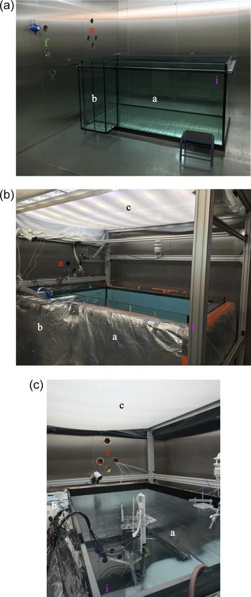
M. Thomas et al.: The Roland von Glasow Air-Sea-Ice Chamber                                                                        1835

technical metrics for designing and interpreting experiments
(Sect. 3.1). We then evaluate how similar our sea ice is to nat-
ural sea ice by comparing our experimental sea ice to natural
sea ice for three key parameters: the extinction of photosyn-
thetically active radiation, the bulk salinity, and the growth
rate (Sect. 3.2).

2     Facility description

2.1    Infrastructure

Our artificial ocean is contained in a cuboid, open-topped,
glass tank (Fig. 1). The internal footprint of the tank is
2.35 m × 1.35 m, and the depth of the tank is 1.17 m. The
glass is 25 mm thick, joined at the edges with silicone resin,
and reinforced with a metal bracketing bar. A smaller cuboid
glass tank (0.5 m × 0.4 m footprint, 1.12 m depth, 12 mm
wall thickness) is joined to the main tank, connected by four
100 mm holes (Fig. 1). This side tank – capped with a lid
– is never allowed to freeze over entirely and so provides a
path for sample lines into the ocean, a path for cables that
does not interfere with the sea-ice–atmosphere interface, and
a free path for water displaced by volume expansion upon
freezing. The main and side tanks have been insulated us-
ing 10 cm of Dow 500A Floormate foam (0.035 W m−1 K−1
thermal conductivity) and 10 cm of foil-backed loft insula-
tion. Heating film (12 V, maximum output 220 W m−2 ) was
placed outside of the glass and within the insulation. The
heating pads and insulation ensure that the dominant cooling
of our experimental system is at the exposed upper interface
rather than through the tank sides. They also prevent sea ice
attaching to our tank walls so that it remains free floating.
Two to four pumps (TUNZE stream 6125, maximum flow
rate of 12 000 L h−1 ) are placed in the main and side tanks to
mix the ocean. The pumps are fixed to the tank walls using
magnets and can be positioned as needed.
   A lighting rack sits at 1.3 m above the tank base (Fig. 1).
Eight UV-B lamps (Philips broadband TL 100 W), eight UV-
A lamps (Philips Cleo performance 100 W), and eight visi-
                                                                   Figure 1. The tank just after installation (a), with all the main fea-
ble LED strips (Fluence solar max) are spaced evenly over
                                                                   tures in place (b), and set up for experiments with visible lighting
the length of the tank. The visible lights can be individually     (c). The labels are consistent with Fig. 3, indicating: a the main
dimmed from 100 % to 10 % of the full output. The LED,             tank, b the side tank, c the lights, e atmosphere sample lines and
UV-A, and UV-B spectra are shown in Fig. 2.                        cables, f ocean sample lines and cables, and i the (0, 0) position of
   The tank and lights are housed in a cold room with a            our sampling coordinate system.
temperature range of −55 to +30 ◦ C. The external footprint
of the cold room is 4.32 m × 4.32 m. The external height is
3.15 m and the internal height is 2.85 m (Fig. 3). The internal    Roxtec ports. The cold room is controlled by a Eurotherm
surfaces of the cold room are stainless steel. Six fans recircu-   nanodac control panel.
late air within the cold room via a compressor. The cold room         The cold room is located in an external laboratory. The
is connected to the outside by double doors, with six 10 cm        control boxes for instrumentation, heating, pumps, cameras,
holes for sample, power, and data lines; one drainage hole;        and valves are all situated adjacent to the cold room. In-
and one ventilation hole. All of these can be closed, and the      struments log to an Envidas Ultimate acquisition system
sample, power, and data lines can be fed in through gas-tight      software for continuous monitoring of the data. Mains or

https://doi.org/10.5194/amt-14-1833-2021                                              Atmos. Meas. Tech., 14, 1833–1849, 2021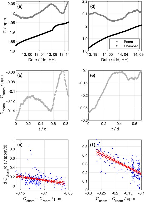
1836                                                             M. Thomas et al.: The Roland von Glasow Air-Sea-Ice Chamber

                                                                        2.2.2   Sea ice

                                                                        Temperature, θ , profiles through the ocean and sea ice are
                                                                        measured using chains of digital thermometers (Table 1).
                                                                                                      1 ◦
                                                                        These have a resolution of 16     C and are calibrated against θ
                                                                        measured by the Sea-Bird 37SIP before each run while they
                                                                        sit in well-mixed water. The chains have 1 to 8 cm resolution
                                                                        and are 10 to 80 cm long. Wireharps (Notz et al., 2005; Notz
                                                                        and Worster, 2008) are used to measure a liquid fraction pro-
                                                                        file, φ, through the sea ice using

                                                                                 γ0 R0
                                                                        φ=                  ,                                         (1)
                                                                             γt (θ, Sbr )Rt

                                                                        where R is the resistance between a given wire pair, γ is the
                                                                        conductivity of the solution between the wire pairs, and the
                                                                        subscripts 0 and t indicate the point in time at which the sea-
                                                                        ice front passes a wire pair and some later point in time. We
                                                                        calculate the bulk sea-ice salinity, Ssi (g kg−1 ), using
Figure 2. Spectral irradiance, Eλ , for the lights in the RvG-ASIC at
                                                                        Ssi = φSbr (θ ),                                              (2)
1 m height and room temperature.
                                                                        where Sbr (θ ) is a the brine salinity. Sbr (θ ) is retrieved from
                                                                        the third-order polynomial presented in Vancoppenolle et al.
18.2 M water supplies (Centra R 200) are available for fill-           (2019) (for natural seawater composition)
ing the tank.
   We use “chamber” to describe the experimental system.                Sbr /(g kg−1 ) = −18.7(θ/◦ C) − 0.519(θ/◦ C)2
When the tank is exposed to the entire cold room, as for all
the experiments presented here, the cold room is the cham-                            − 0.00535(θ/◦ C)3                               (3)
ber.
                                                                        or Rees Jones and Worster (2014) (for NaCl, fit to the data of
2.2     Instrumentation                                                 Weast, 1971),

                                                                        Sbr /(g kg−1 ) = −17.6(θ/◦ C) − 0.389(θ/◦ C)2
The RvG-ASIC has a suite of instruments for carrying out
measurements of the experimental ocean, sea ice, and atmo-                             − 0.00362(θ/◦ C)3 .                            (4)
sphere (Table 1).
                                                                           Our version of the wireharps use two alternating current
2.2.1    Ocean                                                          frequencies, 2 kHz (as used in Notz et al., 2005) and 16 kHz.
                                                                                                                            γ0
                                                                        When using the 2 kHz channel, we calculated γt (θ,S     br )
                                                                                                                                     fol-
The ocean temperature, θo , and conductivity, γo , can be mon-          lowing Notz et al. (2005). When using the 16 kHz channel,
itored by a temperature and conductivity recorder (Sea-Bird             we presume that the electronic double layers driving the con-
                                                                                                                           γ0
MicroCAT SBE 37SIP or Valeport mini CT). θo and γo mea-                 ductivity changes are not present and so take γt (θ,S br )
                                                                                                                                   = 1.
surements are converted to a salinity, So (g kg−1 ), using ei-          We have also deployed fibre optics and photodiode light sen-
ther the GSW toolbox (McDougall and Barker, 2011) for rep-              sors (Hof, 2019, Table 1) in the sea ice and ocean. Fibre op-
resentative ocean salt composition or using equations pre-              tics can be connected to a spectrometer outside of the cold
sented in Naumann et al. (2012) for pure NaCl. A sonar                  room (Ocean Optics USB2000+). The light sensors consist
(Aquascat 1000R) measures the position of the waterline at              of photodiodes, waterproofed in resin, measuring in the blue,
the start of the experiment and the position of the base of the         green, red, and clear. The wavelength range integrated by the
sea ice throughout the experiment. We use the GSW toolbox               photodiodes is, to a good approximation, 400 to 700 nm. The
to calculate the speed of sound for a given So and θo and               response of the photodiodes is negligible to light with wave-
scale the raw sonar output to produce an accurate distance              lengths shorter than 400 nm. At wavelengths above 700 nm,
measurement. We can deploy a Liquicel 1.7 × 5.5 MiniMod-                the response is generally less than 10 % of the maximum
ule in our ocean coupled to a LGR GGA-30r-EP OA-ICOS                    response. Diffusing glass plates sit atop the photodiodes to
laser spectrometer to measure the concentration of dissolved            increase the angle of incidence at which light reaches the
CH4 and CO2 in the ocean without removing water from the                diodes. The data sheet for the photodiodes is given in the
experimental system.                                                    Supplement.

Atmos. Meas. Tech., 14, 1833–1849, 2021                                                    https://doi.org/10.5194/amt-14-1833-2021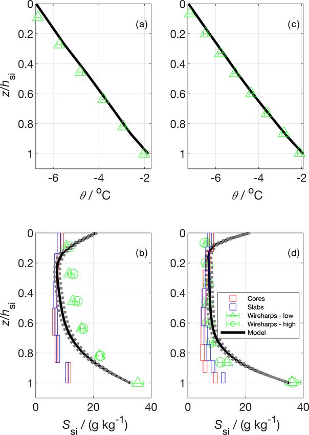
M. Thomas et al.: The Roland von Glasow Air-Sea-Ice Chamber                                                                            1837

Figure 3. Scaled schematic diagram of the cold room. The three panels show orthogonal views from different vantage points. Crosses and
dots indicate air flow away from and towards the viewer, respectively. The lights, shown in grey, are made up of eight sets of visible, UV-A,
and UV-B triplets. The main and side tanks are pale green.

Table 1. Instruments that are generally available in the RvG-ASIC.

    Instrument                                    Parameter                                          Experiment compartment
    Sea-Bird MicroCAT SBE 37-SIP                  conductivity, temperature                          ocean
    DS18B20U digital thermometer                  temperature                                        sea ice and ocean
    Wireharp                                      liquid fraction                                    sea ice
    TCS3472 photodiodes                           irradiance, 400 to 700 nm                          sea ice, ocean, and atmosphere
    Ocean Optics spectrometer (USB2000+)          spectral irradiance                                sea ice, ocean, and atmosphere
    Metcon spectral radiometer                    wavelength-resolved 280 to 650 nm actinic flux     sea ice, ocean, and atmosphere
    LGR GGA-30r-EP                                CO2 and CH4 mole fraction                          atmosphere and equilibrated air
    LGR FGGA                                      CO2 and CH4 mole fraction                          atmosphere and equilibrated air
    Teledyne T200UP                               NO / NO2 / NOx mole fractions                      atmosphere
    Teledyne T200U                                NO / NOy mole fractions                            atmosphere
    Teledyne T400                                 O3 mole fraction                                   atmosphere
    Teledyne T700U                                dynamic dilution calibrator with ozone generator
    Teledyne T701H                                zero air generator
    WS600-UMB                                     temperature, wind speed, humidity                  atmosphere
    Camsecure, underwater camera                  video                                              ocean
    4K HD video camera                            video                                              atmosphere

https://doi.org/10.5194/amt-14-1833-2021                                                       Atmos. Meas. Tech., 14, 1833–1849, 2021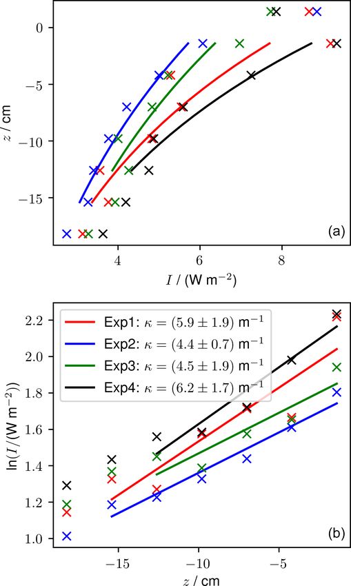
1838 M. Thomas et al.: The Roland von Glasow Air-Sea-Ice Chamber
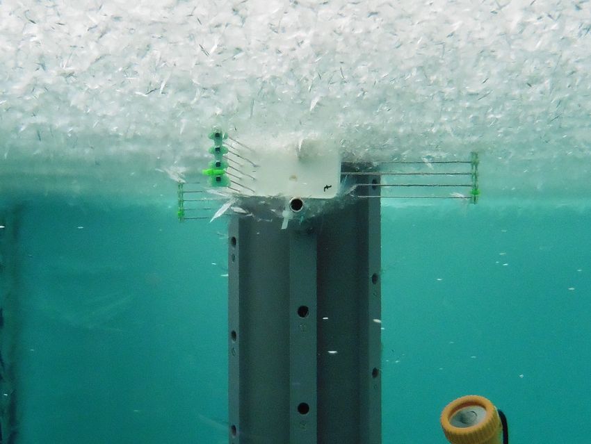
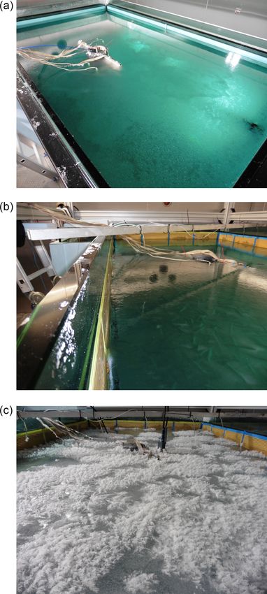
2.2.3 Atmosphere 2.3.2 Growth phase
The water circulation rate and the atmospheric temperature
The temperature, wind speed, and relative humidity of our determine the nature of the sea ice (Naumann et al., 2012).
atmosphere are measured using a weather station (WS600- Nilas will grow in quiescent water. In circulating water, a
UMB). Two Los Gatos Research (LGR) greenhouse gas anal- layer of grease ice will form that subsequently consolidates.
ysers measure CO2 , CH4 , and H2 O mole fractions in the at- When the growth temperature is less than −25 ◦ C, frost flow-
mosphere and can also analyse the air stream of the Liquicel ers form on the sea-ice surface (Fig. 4). By running the heat-
equilibrator (Table 1). A Teledyne T200UP measures NO and ing pads between the main tank and insulation, we are able
NOx and a T200U measures NO and NOy . A Teledyne T400 to maintain free-floating sea ice to 20 cm thickness with no
measures ozone. There is also a zero air generator (T701 visible water gap at the tank sides. We have verified that the
H, Teledyne) and a T700U dynamic dilution calibrator with sea ice is free-floating in several experimental runs by gently
ozone generator. pressing the corner of the sea ice and noting that it bobs. With
no, or insufficient, side heating, the sea ice attaches to the
2.3 Experimental protocols tank sides and the surface floods (e.g. Rysgaard et al., 2014),
resulting in a shiny, liquid surface layer. Sea ice, fast to the
tank walls, has been grown up to 25 cm thickness and could
Protocols vary widely between experiments. Here, we pro- potentially be grown thicker. With insufficient side heating
vide a typical protocol to help future users visualise the fa- and insulation, the ocean tends to supercool (Fig. 5). When
cility and plan experiments. the ocean supercools, ice grows on the tank sides and instru-
ments, causing problems with measurements and potentially
damaging equipment. Growth phases typically last for a few
2.3.1 Set-up phase days to a few weeks.
We set up instrumentation in a dry, clean tank. Sea-ice instru- 2.3.3 Sampling protocols
mentation is attached to poles that are free to rise in the verti-
Underlying water may be sampled throughout, providing the
cal as sea ice grows and floats. Ocean and atmosphere instru-
volume is replaced. We sample sea ice either by taking cores
mentation and sample lines are mounted in a fixed position.
using a 7.5 cm diameter Kovacs ice corer or using the pro-
The nature of the experiment will determine the state of the
cedures outlined by Cottier et al. (1999) to extract sea-ice
tank sides and base. For optical experiments (Sect. 3.2.1), the
“slabs”. Sea-ice cores have a known bias, particularly prob-
tank’s inner surfaces should be covered to simplify the light
lematic in young sea ice, as brine is lost from the permeable
field. We use mirrored sides and a matt black base to approxi-
sea ice near the ocean interface. The method of Cottier et al.
mate infinite lateral boundary conditions and a non-reflective
(1999) seeks to minimise this bias by collecting sea-ice sam-
ocean (Fig. 1).
ples that are still floating and then freezing the sample and
To fill the tank, we add 100 kg of salt and mix this with
surrounding ocean at −40 ◦ C to immobilise the brine before
tap or 18.2 M water. The salt can be pure NaCl (used
processing the sample. The method of Cottier et al. (1999)
for Sect. 3.1.2 and 3.2.1) or a natural sea salt composition
becomes difficult and time consuming when sea ice is thicker
(Tropic Marin sea salt classic, used for Sect. 3.2.2). The tank
than around 25 cm due to limitations of the power tools used
takes around 18 h to fill with de-ionised water or a few hours
to extract the slabs and the weight of the slabs. We cut cores
from the tap, and 100 kg of salt dissolves in a few hours under
and slabs into discrete vertical profiles using a bandsaw with
vigorous circulation by the pumps. Alternatively, real sea wa-
a precleaned blade at −25 ◦ C.
ter can be delivered to the tank. Filling the tank to 1 m gives
an ocean volume of around 3.2 m3 . Once the tank is full, we
begin to cool the water. The tank surface can be covered at 3 Characterisation of experimental system
this stage to reduce evaporation. With an atmospheric tem-
perature of −20 ◦ C, and an uncovered tank, the temperature We now turn to a characterisation of our experimental sys-
of 3.2 m3 of ocean drops by around 1 ◦ C every 4 h. If the ex- tem. First, in Sect. 3.1, we quantify several parameters re-
periment requires an isolated cold room atmosphere, the cold garding the technical capabilities of the facility: the exchange
room is sealed at this stage. Sea-ice growth can be initialised rate between the chamber and the outside, the mixing rate of
by continuing to cool under constant temperature and vigor- the water in the tank, and the variability in the light field.
ous circulation. Alternatively, once the water is within a few In doing so, we aim at providing valuable information to
tenths of a degree of its freezing point, turning the pumps to help plan and interpret future studies. Next, in Sect. 3.2, we
a low setting, or off, initialises sea-ice growth within a few present measurements of our experimental sea ice to quantify
minutes. As a rule of thumb, it takes one full week to go from the extinction of PAR (λ = 400 to 700 nm), the bulk salinity,
a dry tank to first sea ice. and the growth rate of our experimental sea ice. The goal
Atmos. Meas. Tech., 14, 1833–1849, 2021 https://doi.org/10.5194/amt-14-1833-2021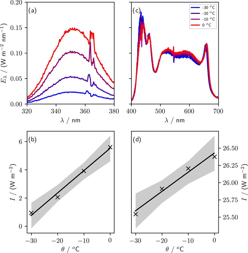
M. Thomas et al.: The Roland von Glasow Air-Sea-Ice Chamber                                                                         1839

                                                                       Figure 5. A view of a supercooled ocean. Frazil ice crystals are
                                                                       floating upwards in the water column (white flecks) and have nucle-
                                                                       ated on wireharps well ahead of the advancing sea-ice–ocean inter-
                                                                       face.

                                                                       of this section is to investigate how similar our laboratory-
                                                                       grown sea ice is to natural sea ice with respect to these im-
                                                                       portant characteristics.

                                                                       3.1     Technical characterisation

                                                                       3.1.1    Quantifying the cold room air exchange rate

                                                                       For most experiments, it is desirable to have the sea-ice–
                                                                       atmosphere interface exposed to the bulk air within the cold
                                                                       room. Leaving the atmosphere of the tank uncapped ensures
                                                                       that the temperature of the atmosphere overlying the sea ice
                                                                       is responsive to the cold room atmosphere. When the at-
                                                                       mosphere is contained by some headspace, the temperature
                                                                       tends to be much warmer than the cold room (e.g. Loose
                                                                       et al., 2011). Here, we quantify the degree to which the cold
                                                                       room can be sealed from the outside by deriving the air ex-
                                                                       change rate coefficient, k, and time constant, τl , of CH4 ex-
                                                                       changing between the cold room to the outside (Fig. 6).
                                                                          To do so, we sealed the cold room and left the tank dry.
                                                                       We then diluted the chamber air by filling it with N2 gas.
                                                                       We performed two dilutions, the first at around 18:00 LT
                                                                       on 12 February 2019 and the other at around 16:00 LT on
                                                                       13 February 2019. The CH4 concentration in the chamber,
                                                                       Ccham , was monitored using an LGR (GGA type, Table 1),
                                                                       where measured air was returned to the cold room in a closed
                                                                       loop (Fig. 6a and d). The dilution reduced Ccham by around
                                                                       0.1 ppm in both dilution periods. We stopped the dilution by
Figure 4. Grease ice (a) grown under pumping, nilas (b) grown in
quiescent conditions, and a frost flower field (c) grown in the RvG-
                                                                       stopping the N2 flow, at which point the chamber was sealed
ASIC.                                                                  to the best of our ability. We measured the CH4 concentra-
                                                                       tion in the outer laboratory, Croom , throughout using an LGR
                                                                       (FGGA type, Table 1), and we used the difference between
                                                                       Ccham and Croom as the concentration gradient between the
                                                                       chamber and the outside (Fig. 6b and e). Before the exper-

https://doi.org/10.5194/amt-14-1833-2021                                                  Atmos. Meas. Tech., 14, 1833–1849, 2021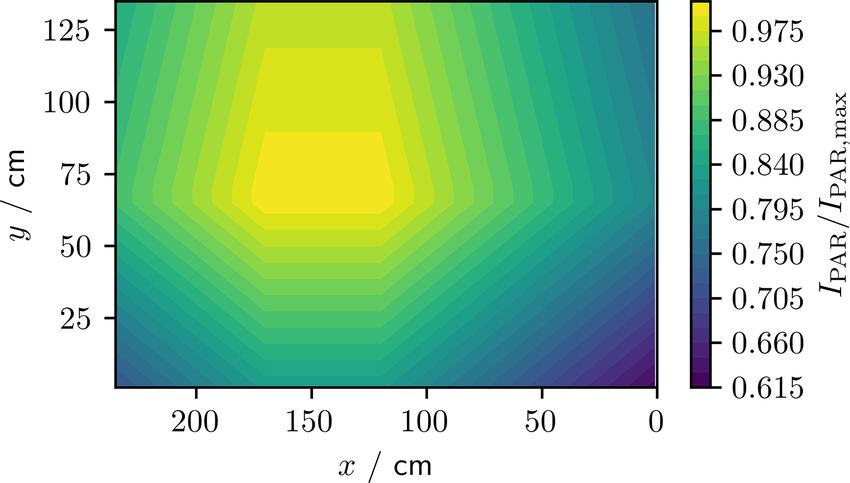
1840                                                              M. Thomas et al.: The Roland von Glasow Air-Sea-Ice Chamber

                                                                         dCcham
                                                                           dt    and Ccham − Croom , as well as the linear fit. We de-
                                                                         rived k = (1.5±0.3) d−1 and k = (1.5±0.1) d−1 for the first
                                                                         and second experiments, respectively. Taking the mean k of
                                                                         the two experiments, the air exchange time constant is then
                                                                         given by

                                                                         τl = 1/k = (0.66 ± 0.07) d.                                  (6)

                                                                         The physical interpretation of this τl is that the concentration
                                                                         difference between the sealed chamber and the outside will
                                                                         reduce by a factor of e every (0.66 ± 0.07) d.

                                                                         3.1.2    Quantifying the tank mixing rate

                                                                         For some experiments, it may be necessary to spike the ocean
                                                                         with a chemical. We may, in such cases, want to know when
                                                                         the water will be well mixed with respect to our spike. Simi-
                                                                         lar to the air exchange rate (Sect. 3.1.1), the degree to which
                                                                         the chemical has mixed can be quantified using a time con-
                                                                         stant, τm . To derive this time constant, we spiked our tank
                                                                         with saturated NaCl solution by injecting it near the tank base
                                                                         and observed the conductivity of our ocean over time as it
                                                                         mixed under the action of three pumps (Fig. 7). The temper-
                                                                         ature of the ocean was stable to within 0.02 ◦ C for the hour
                                                                         time period over which we monitored both spikes, so we ex-
                                                                         pect the salinity to be linearly related to the conductivity. The
                                                                         conductivity of the ocean, γo , can then be described by
                                                                                      t
                                                                         γo (t) = e− τm (γo (t0 ) − γo,∞ ) + γo,∞ ,                   (7)
Figure 6. Data from experiments to determine the chamber air ex-
change rate. Panels (a) to (c) and (d) to (f) show data from the first   where γo,∞ is the maximum ocean conductivity obtained af-
and second experiments, respectively. The top panels (a and d) show      ter the spike and t0 is the time of the spike. Fitting an ex-
the measured CH4 concentrations in the chamber and the lab out-          ponential curve to a manually defined spike period for the
side. Panels (b) and (e) show the concentration difference between       two runs produces τm = (4.2 ± 0.1) min (run 1) and τm =
the chamber and the lab outside. Panels (c) and (f) show the linear      (4.1 ± 0.1) min (run 2). We take the mean of the individ-
regressions constructed using Eq. (5). Blue dots show individual         ual experiments to characterise our mixing rate, such that
data points. The red lines show the best fit and 95 % confidence         τm = (4.2 ± 0.1) min. The tank should therefore mix to more
intervals of the linear regression of dCdt
                                        cham against C
                                                       cham − Croom .    than 99% of the perfectly mixed concentration in less than
The gradient of the linear regression corresponds to the air exchange    30 min.
rate coefficient, −k. For the first experiment, k = (1.5 ± 0.3) d−1 ,
and for the second experiment, k = (1.5 ± 0.1) d−1 .
                                                                         3.1.3    Quantifying light-field variability

                                                                         Producing a homogeneous light field in a laboratory envi-
iment, the two LGR instruments measured the same air for
                                                                         ronment can be difficult, because shading and reflection can
30 h. The offset between them was (6.4±0.2) ppb. This offset
                                                                         cause heterogeneities. The intensity of our lights is also tem-
was added to Croom values to make the measurements from
                                                                         perature dependent, which is particularly important in the
the two LGR instruments consistent. Data were averaged in
                                                                         RvG-ASIC given the wide range of experimental tempera-
5 min bins. We modelled the exchange rate as a first-order
                                                                         tures. In this section, we aim to characterise our light field,
process,
                                                                         both in terms of lateral heterogeneity and with changes in
dCcham                                                                   temperature.
       = −k(Ccham − Croom ).                                      (5)       To assess the spatial variability, we measured PAR (photo-
  dt
                                                                         synthetically active radiation, λ = 400 to 700 nm) across the
We approximate dCdtcham for each measurement interval using              tank area at 1 m height (Fig. 8). These measurements were
the difference in Ccham between adjacent data points over                made using a LI-COR LI-1800 spectroradiometer integrated
the 5 min between those data. Panels c (experiment 1) and                from 400 to 700 nm. The PAR irradiance, IPAR , at 1 m above
f (experiment 2) of Fig. 6 show the relationship between                 the tank base and 25 ◦ C was generally within 80 % of the

Atmos. Meas. Tech., 14, 1833–1849, 2021                                                    https://doi.org/10.5194/amt-14-1833-2021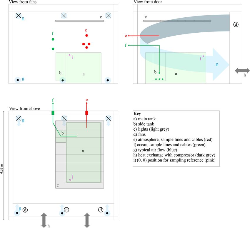
M. Thomas et al.: The Roland von Glasow Air-Sea-Ice Chamber                                                                     1841

                                                                       lights are more strongly temperature dependent, with irradi-
                                                                       ance dropping by 83 % between 0 and −30 ◦ C, while PAR
                                                                       irradiance dropped by just 3 %.

                                                                       3.2     Sea-ice characterisation

                                                                       3.2.1    Determining PAR extinction coefficients in sea ice

                                                                       The importance of understanding the sea-ice light field is
                                                                       critical as thinner, fresher, and more transient sea ice be-
                                                                       comes more common. Even thin sea ice without snow cover
                                                                       impacts the transmission of PAR to the ocean and has been
                                                                       seen to accumulate algal biomass rapidly within the sea
                                                                       ice (Taskjelle et al., 2016). Photochemical production rates
                                                                       within sea ice are also dependent upon sea-ice optical prop-
                                                                       erties. Irradiation through sea ice has been postulated as a
Figure 7. Experiments to determine the mixing time constant of
                                                                       source of OH radicals (King et al., 2005) and as a stressor of
our tank, τm . Saturated NaCl solution was spiked into the tank and
mixed under pumping. The conductivity of the bulk water is shown       diatoms that may lead to iodine production from algae (Küp-
by the grey markers. The coloured lines show the prediction of         per et al., 2008).
Eq. (7) using τm fit to the data. In reality, the spike in run 2 was      The rationale for UV–Vis illumination experiments in a
a few hours after run 1, but the times for the two spikes have been    controlled sea-ice facility is twofold: first, to allow for ex-
matched for ease of comparison.                                        periments investigating the optical properties of sea ice (and
                                                                       potentially other mediums such as snow); second, to allow
                                                                       simple experimental simulations of photochemistry or biol-
                                                                       ogy occurring in the sea ice, atmosphere, or ocean. The ex-
                                                                       tinction coefficient, κ, of PAR in sea ice quantifies the rate
                                                                       of attenuation of PAR with depth. Here, we present measure-
                                                                       ments of κ for sea ice grown in the RvG-ASIC and compare
                                                                       those to previously reported values.
                                                                          To quantify κ in our experimental sea ice, we performed an
                                                                       experiment using visible lighting, measuring a vertical pro-
                                                                       file of irradiance using eight photodiodes (Sect. 2.2.2). The
                                                                       photodiodes respond dominantly to 400 to 700 nm light, and
                                                                       our lighting provides irradiance predominantly in the 400
                                                                       to 700 nm range, so κ as measured by the photodiodes is a
Figure 8. Normalised PAR (λ = 400 to 700 nm) irradiance across         good estimate of κ for PAR. The tank sides were covered
the footprint of the tank at 1 m height. The (0, 0) cm coordinate      with mirrored tape to approximate infinite lateral boundary
corresponds to the pink asterisk in Fig. 3.                            conditions, and the tank base was covered with a matt black
                                                                       plastic sheet to approximate no reflection from the ocean. A
                                                                       3 mm opal polycarbonate sheet was placed 20 cm below the
maximum recorded intensity, IPAR,max , but dropped as low              light rack to create a diffuse light field, and black curtains
as 60 % in one corner of the tank.                                     were draped between the lights and the tank to prevent re-
   We measured spectra for UV (UV-A lighting, 320 to                   flection off the shiny cold room walls (Fig. 1). We deployed
380 nm) and PAR (LED lighting, 400 to 700 nm) at −30,                  the photodiodes with 2.8 cm vertical resolution. The sensors
−20, −10, and 0 ◦ C using a USB2000+ spectrometer ref-                 were calibrated pre-deployment against the Metcon spectral
erenced against the Metcon spectral radiometer (Fig. 9).               radiometer. Before each experimental run, while sitting in
To quantify the temperature sensitivity, we integrated the             open water, an additional correction was applied to the in
UV and PAR spectral irradiance over their respective wave-             situ sensor output to bring it in line with depth profiles mea-
length ranges (320 to 380 nm and 400 to 700 nm, respec-                sured using the spectral radiometer. We performed four ex-
tively). The maximum irradiance was 5.6 W m−2 for UV and               periments at growth temperatures of −10, −20 (two runs),
26.4 W m−2 for PAR, both at 0 ◦ C. The temperature sensi-              and −30 ◦ C (Table 2). For each run, we present vertical light
tivity of the irradiance was (0.16 ± 0.01) W m−2 ◦ C−1 for             profiles taken at the end of the growth phase, as well as κ
UV and (0.028 ± 0.003) W m−2 ◦ C−1 for PAR. The UV-A                   calculated by two methods (Fig. 10 and Table 3). Method A

https://doi.org/10.5194/amt-14-1833-2021                                                 Atmos. Meas. Tech., 14, 1833–1849, 2021
1842 M. Thomas et al.: The Roland von Glasow Air-Sea-Ice Chamber
Figure 9. Sensitivity of lights to variations in temperature. Panels (a) (UV) and (c) (PAR) show spectra taken at four temperatures between
0 and −30 ◦ C. Panels (b) (UV, 320 to 380 nm) and (d) (PAR, 400 to 700 nm) show the irradiance, I (integrated spectral irradiance over the
respective wavelength ranges), at each temperature, θ . The gradient of the regression of I against θ is (0.028 ± 0.003) W m−2 ◦ C−1 for PAR
and (0.16 ± 0.01) W m−2 o C−1 for UV.
(Ehn et al., 2004; Kauko et al., 2017) uses ice. Previous studies, compared to our measurements in Ta-
ble 3, have calculated κ by iteratively solving the Dunkle and
I (+1.4 cm) Bevans (1956) photometric model such that κ provides the
κ = ln (1 − ζs ) /z. (8)
I (z) best fit to measured albedo and transmission (Perovich and
Grenfell, 1981) – which we call method C.
The depth, z, is chosen to be the shallowest sensor not yet Measured light profiles taken at the end of four experi-
frozen into the sea ice, and spectral reflectance, ζs , assumed ments are shown in Fig. 10. The thickness varied by up to
to be 0.05. Ehn et al. (2004) measured κ ranging from 3.1 3 cm between the four experiments. At the end of the exper-
to 4.7 m−1 in 24 to 28 cm thick sea ice (Table 3). Kauko iments, runs 1 and 2 had six sensors frozen into the sea ice
et al. (2017) measured κ ranging from 2.9 to 4.7 m−1 in 17 and experiments 3 and 4 had five sensors frozen into the sea
to 27 cm thick sea ice. For method B, we also calculated κ by ice. The light intensity at 1.4 cm above the sea ice was be-
fitting a linear model to tween 7.7 and 8.9 W m−2 and reduced to between 2.8 and
3.6 W m−2 at 18.2 cm depth. For experiments 1 and 4, the
ln(I /(W m−2 )) = −κz + c, (9) shallowest frozen sensor measured higher intensity than the
sensor above the sea ice, which is a phenomenon that was
similar to (Marks et al., 2017). Equation (9) represents a light
predicted by Jiang et al. (2005) and that is due to the change
field decaying exponentially with depth. While methods A
in refractive index across the air–ice interface.
and B both provide estimates of κ, they do so in different
Using method A, our calculated κ ranges from 3.7 (ex-
ways, with method A using measurements external to the sea
periment 4) to 6.1 m−1 (experiment 2). Using method B, our
ice while method B uses only measurements within the sea
Atmos. Meas. Tech., 14, 1833–1849, 2021 https://doi.org/10.5194/amt-14-1833-2021M. Thomas et al.: The Roland von Glasow Air-Sea-Ice Chamber 1843
Table 2. Overview of experiments used to calculate with PAR extinction coefficients. θatm gives the mean atmospheric temperature during
the experiment. ψψ is the mean relative humidity during the experiment, with ψ representing humidity and the subscript sat indicating
sat
saturation. tf gives the duration of the freeze up period. hsi gives the maximum thickness attained, at which point κ was measured.
ψ
Experiment θatm / ◦ C ψsat tf / d hsi / cm Surface
characteristics
1 −18.9 ± 0.4 0.59 ± 0.05 6.1 18 Flooded
2 −26.6 ± 0.9 0.59 ± 0.03 5.1 18 Frost flowers
3 −9.2 ± 0.9 0.52 ± 0.03 10.1 15
4 −18.0 ± 0.5 0.60 ± 0.05 7.0 15
Table 3. Comparison of PAR extinction coefficients (κ, wavelength range 400 to 700 nm) produced by this work and by different studies.
Experiment θatm / ◦ C hsi / cm κ / m−1
A B C
This work, Exp. 1 −18.9 ± 0.4 18 5.3 5.9 ± 1.9
This work, Exp. 2 −26.6 ± 0.9 18 6.1 4.4 ± 0.7
This work, Exp. 3 −9.2 ± 0.9 15 4.1 4.5 ± 1.9
This work, Exp. 4 −18.0 ± 0.5 15 3.7 6.2 ± 1.7
Nice1 −10 to −20 17 to 27 2.9 to 4.7
Santala Bay, Finland2 < −5 to 5 24 to 28 3.1 to 4.7
Laboratory3 −10 28 2.5
Laboratory3 −30 28 3
Laboratory4 −15 40 3 to 10
1 Kauko et al. (2017); 2 Ehn et al. (2004); 3 Perovich and Grenfell (1981); 4 Marks et al. (2017).
A – Eq. 8. B – Eq. 9. Values from this work are broadband κ , while the range of values given for Marks
et al. (2017) cover a range of κ at wavelengths between 350 and 650 nm. C – Dunkle and Bevans (1956)
model iteratively solved.
calculated κ ranges from 4.4 (experiment 2) to 6.2 m−1 (ex- measured bulk salinities ranging from around 35 g kg−1 at
periment 4). For both methods, the range of κ observed in the sea-ice–ocean interface to around 4 g kg−1 in the interior.
our tank overlaps with the range of κ observed previously Mean salinities decreased from around 35 towards 10 g kg−1
for thin sea ice. These results build confidence that the RvG- (experiment 1) and around 15 g kg−1 (experiment 2). Here,
ASIC is a useful tool for future biological or photochemical we present bulk salinities for sea ice grown in the RvG-ASIC,
experiments in young sea ice and validate this particular ex- comparing it to the range of salinities observed in nature.
perimental setup for experiments involving visible light. Quantifying the vertical bulk salinity profile in sea-ice cores
– the most common sea-ice sampling methodology – is dif-
3.2.2 Estimating sea-ice bulk salinity ficult due to the known bias during coring of brine loss and
bulk salinity underestimation. Several other methodologies
Bulk salinity is a sea-ice state variable that, when measured have been proposed. Cottier et al. (1999) present a destruc-
alongside temperature, can allow for estimation of the sea- tive sampling methodology that attempts to prevent brine
ice liquid fraction. Growing sea ice desalinates rapidly by loss upon sampling (Sect. 2.3.3). Notz et al. (2005) present
gravity drainage (Notz and Worster, 2008). The bulk salin- instrumentation, called a wireharp, to quantify the in situ
ity of natural, young sea ice has been measured using cores bulk salinity profile. Several groups have presented grav-
(Weeks and Lee, 1962) and wireharps (Notz and Worster, ity drainage parameterisations that quantify the bulk salin-
2008). Weeks and Lee (1962) sampled young sea ice in North ity profile during sea-ice growth (Griewank and Notz, 2013;
Star Bay, Greenland, in growing sea ice between 5 and 23 cm Rees Jones and Worster, 2014; Cox and Weeks, 1988; Van-
thick. Salinities ranged from around 5 to 20 g kg−1 verti- coppenolle et al., 2010; Turner et al., 2013; Jeffery et al.,
cally with mean salinities decreasing from 20 g kg−1 early in 2011), noting that gravity drainage is the dominant process
the growth to around 10 g kg−1 after 10 d. Notz and Worster redistributing salt in growing sea ice (Notz and Worster,
(2008) cut a hole in Arctic sea ice and measured the salin- 2009).
ity profile, in situ, as it refroze up to 17 cm thickness (the We performed two sea-ice growth experiments in the RvG-
depth range of their instrument). Over two experiments, they ASIC and estimated the sea-ice salinity by (1) constructing a
https://doi.org/10.5194/amt-14-1833-2021 Atmos. Meas. Tech., 14, 1833–1849, 20211844 M. Thomas et al.: The Roland von Glasow Air-Sea-Ice Chamber
of the three sets of tuning parameters presented in Griewank
and Notz (2015) (Table 4). The model is forced by measured
temperature profiles and sea-ice thickness in lieu of mod-
elled thermodynamics (Fig. 11). Cores and slabs were ex-
tracted according to Sect. 2.3.3 and sectioned vertically into
1 to 2 cm layers. Ice samples were melted and placed in a
20 ◦ C thermostatic bath. Conductivity was measured using a
conductivity probe (Orion) and calibrated with certified ref-
erence material (Thermo Scientific Eutech Handheld Meters
Calibration Solution). Bulk salinity was derived using the
GSW toolbox (McDougall and Barker, 2011). We discarded
three discrete samples (one from the cores and two from the
slabs for run 1) because of punctured sample bags. A single
wireharp profile was taken in the middle of the tank and used
to derive φ and Ssi (Eqs. 1 and 2).
The mass balance was constructed by conservation of
mass and salt from the start of each run (t0 ) to the final sam-
pling (tend ). The conservation of mass gives
msys = mo + msi , (10)
where m is mass, and the subscripts sys, o, and si indicate
the experimental system, ocean, and sea-ice compartments,
respectively. Noting that msys = mo (t0 ), the conservation of
salt at the end of the experiment (tend ) gives
msys So (t0 ) = mo So (tend ) + msi S si . (11)
Our desired variable is the vertically integrated bulk sea-ice
salinity, S si , which we recover by substituting Eq. (10) into
Figure 10. Irradiance profiles (a) and linear regressions of Eq. (11), giving
ln(I /W m−2 ) vs. z (b) used to produce extinction coefficients
(Eqs. 8 and 9) from the final profile of the freezing period. The S si = r1S + So (tend ), (12)
legend in (b) gives the extinction coefficient for a given profile with
1 standard error. where
1S = So (t0 ) − So (tend ) (13)
salt and mass budget, (2) taking sea-ice cores, (3) taking sea- and r gives the ratio of the mass of the experimental system
ice slabs (Cottier et al., 1999), (4) using a wireharp (Notz to the mass of the sea ice at final sampling, such that
et al., 2005), and (5) using the Griewank and Notz (2013)
gravity drainage parameterisation. Our artificial ocean was ho (t0 )ρo (t0 )
r= . (14)
composed of Tropic Marin sea salt and deionised water such hsi ρsi
that So = (31.3±0.1) g kg−1 . We grew free-floating sea ice to The error on Eq. (12) was calculated by Gaussian propaga-
(11.0 ± 0.9) cm (run 1) and (16.4 ± 2.7) cm (run 2) thickness tion, such that
(mean and standard deviation of measured ice core thick- s
ness). Measurements of sea-ice temperature, thickness, and
u(r) 2
u(1S) 2
the initial ocean salinity were used to force the model, which u(S si ) = r 2 1S 2 + + u(So )2 , (15)
r 1S
has been used previously to model experiments in the RvG-
ASIC (Garnett et al., 2019; Thomas et al., 2020). We used the where u gives the uncertainty of the individual terms. The
Griewank and Notz (2013) gravity drainage parameterisa- dominant uncertainty, accounting for > 95 % of u(S si ), prop-
tion, because it performed well in previous studies (Thomas agates from u(r) and derives chiefly from the variability in
et al., 2020) and has tuning parameters shown to perform measured hsi . The errors on So (t0 ) and So (tend ) are highly
well for Arctic field data (Griewank and Notz, 2015). The correlated given the stability of the salinity sensor over the
model has two tuning parameters: the critical Rayleigh num- short duration of the experiment, and as such u(1S)
ber, Rac , and the desalination strength, α. We estimate an 0.01 g kg−1 and has a negligible impact on u(S si ). The sen-
uncertainty on the modelling by running the model for each sitivity of S si to our choice of ρsi is around 0.02 (g kg−1 )
Atmos. Meas. Tech., 14, 1833–1849, 2021 https://doi.org/10.5194/amt-14-1833-2021M. Thomas et al.: The Roland von Glasow Air-Sea-Ice Chamber 1845
and no more correction to the profile is necessary. For sim-
plicity, and because the high-frequency channel has not yet
registered ice growth in the deepest run 1 sensor, we proceed
by discussing only the low-frequency channel. For both runs,
and for all profiles, there is a salinity maximum near the sea-
ice–ocean interface (z = hsi ). The model and the wireharps
converge towards So as z approaches hsi . The cores and the
slabs produce the lowest Ssi near this lower interface, with
the slabs giving higher Ssi relative to the cores in this re-
gion in run 2. For run 1, the wireharps generally measure the
highest Ssi , the cores and slabs are similar and measure the
lowest Ssi , and the model is intermediate. For run 2, the cores,
slabs, wireharps, and model are generally consistent between
z/hsi = 0.6 to 0.1. Near the upper interface, the model pre-
dicts higher Ssi than the measurements, and the wireharps
give the lowest Ssi . For run 1, the cores and slabs are con-
sistent throughout, but the wireharps, model, and discrete
samples generally disagree. Towards the sea-ice–atmosphere
interface (z = 0), the wireharps produce minima in Ssi . The
cores and slabs show an ≈ 1 g kg−1 increase in Ssi for the
shallowest layer relative to the layer below, forming a C-
shaped profile. Modelled Ssi at z = 0 is around 10 g kg−1
greater than in the interior, forming a C-shaped profile that
is more pronounced than in the discrete samples at both in-
terfaces. The difference in θ between the wireharps and the
forcing is at most 0.2 ◦ C which, depending on Sbr , translates
to a 2 % to 3 % difference in Ssi .
The mass balance produces S si = (11.0 ± 2.0) g kg−1 (run
1) and S si = (11.0 ± 4.1) g kg−1 (run 2) (mean and standard
Figure 11. Vertical temperature (a and c) and bulk salinity profiles deviation, Table 4). These values represent the vertically in-
(b and d) for two experimental runs. In (a) and (c) the model tem-
tegrated bulk sea-ice salinity, averaged over the tank foot-
perature shows the model forcing, which was produced using mea-
print. We compare the measurements and model to the mass
sured temperature profiles; panels (b) and (d) show salinity esti-
mated from cores, slabs (Cottier et al., 1999), wireharps (Notz et al., balance by calculating S si for the profile produced by each
2005), and a gravity drainage model. The horizontal box length method at the end of each run. For the cores and slabs, we
shows the median 1 standard deviation from repeat measurements first averaged the individual layer measurements for each
at a given depth (cores and slabs), and the vertical box length shows sample and then took the average of these samples to be S si .
the depth covered by the sample layer. Wireharp errors were cal- For the wireharps, we linearly interpolated measured Ssi to
culated using methodology presented in Zeigermann (2018). The the midpoint between each measurement, and took the mean
model used the Griewank and Notz (2013) gravity drainage param- of these interpolated Ssi to produce S si . In this way, we more
eterisation with tuning parameters taken from Griewank and Notz closely approximate the treatment of the cores and slabs, for
(2015). The solid line represents their best estimate tuning parame- which the edge of the bottommost layer is at z = hsi . Model
ter set. The dotted bounds on the model show output using two other
S si is the mean of the Ssi of individual model layers. The
plausible sets of tuning parameters presented in Griewank and Notz
cores and slabs perform similarly, underestimating the mass
(2015).
balance for each run. The wireharps overestimate the mass
balance in run 1 and capture the run 2 mass balance to within
1 standard deviation. The best estimate model S si is consis-
/ (kg m−3 ), such that a 20 kg m−3 increase in ρsi causes a tent with the mass balance for both runs.
0.4 g kg−1 increase in our estimated S si , which is well within The underestimation of S si by the cores (Table 4) high-
our uncertainty bounds. lights a known bias in sea-ice core bulk salinity measure-
We first turn to the vertical profiles of Ssi (Fig. 11). For ment, which is that of brine loss upon sampling. This bias is
both runs, the wireharp profile at low frequency including apparent in the vertical profiles (Fig. 11), where cores give
the electrical double-layer correction proposed by Notz et al. the lowest estimates of Ssi in the lower third of the pro-
(2005) is very similar to the high-frequency wireharp profile file, which we expect to be most affected by brine loss. The
without such correction. This confirms that at higher frequen- slabs perform similarly to the cores, potentially due to brine
cies the impact of the double layer becomes less important, drainage during the shock freezing process. The slabs retain
https://doi.org/10.5194/amt-14-1833-2021 Atmos. Meas. Tech., 14, 1833–1849, 20211846 M. Thomas et al.: The Roland von Glasow Air-Sea-Ice Chamber
more brine than the cores in run 2, as shown by their higher
Ssi in the lower portion and their higher S si . Previous work
has tuned gravity drainage parameterisations to slab Ssi mea-
surements (Thomas et al., 2020), and these tuning parame-
ters may therefore be biased to predict too much desalination.
The wireharp performance is more variable, overestimating
S si in run 1 and capturing the mass balance in run 2. The
performance of the model, forced with measured θ and hsi ,
solely reflects the gravity drainage parameterisation and its
tuning (Griewank and Notz, 2013, 2015), incorporating min-
imal error from thermodynamics. Only the model captures
the mass balance for both runs. The mass balance is, for both
runs, within the range of young sea-ice salinities observed in
nature (Weeks and Lee, 1962; Notz and Worster, 2008).
3.2.3 Quantifying sea-ice growth rates
The growth rate of sea ice depends on the balance of fluxes at
the sea-ice–ocean interface, the thermal conductivity of the Figure 12. Thickness measured from temperature profiles dur-
sea ice (K), sea-ice thickness hsi , and the absolute sea-ice ing the experiments presented in Sect. 3.1.3 and modelled using
surface temperature (Ts ). Growth rates in young sea ice have Eq. (16).
been observed to range from 2.7 to 12 cm d−1 (Wakatsuchi
and Ono, 1983). Following Stefan (1889), the change in sea-
ice thickness is modelling and measuring the growth rate of the four exper-
dhsi imental runs presented in Sect. 3.2.1 and Table 2 (Fig. 12).
= −FC /(ρi L), (16) When the temperature of a sensor at depth z dipped by 0.1o C
dt
below the water temperature for 30 min, we took hsi = z.
where L gives the latent heat of fusion of water, and FC gives For each run, we forced the sea-ice growth and desalination
the vertical conductive heat flux through the sea ice. FC , was model (Sect. 3.2.2, Thomas et al., 2020) with the mean Ta and
calculated using ψ during the freezing period, as measured by the weather sta-
tion (Table 2). Incoming shortwave flux, FS , was taken to be
FC = K(Ts − Tf )/hsi . (17)
8 W m−2 based on measurements of PAR just above the sea-
The vertically averaged thermal conductivity is K = Ki (1 − ice surface (Sect. 3.1.3). In this case, Eqs. (16) to (20) were
φ) + Kbr φ, where the subscripts i and br indicate pure ice used to calculate Ts , hsi , and the internal sea-ice temperature
and brine, respectively. Tf is given by the salinity-dependent profile. Tf was calculated from the salinity-dependent freez-
freezing point of the ocean, and Ts is found by iteratively ing point of the model ocean.
solving the surface energy balance of the sea ice Over the four experiments, measured growth rates range
from 2 cm d−1 (experiment 3, highest air temperature) to
FL↓ − FL↑ + FS + FC = 0, (18) 4 cm d−1 (experiment 2, lowest air temperature). These
growth rates are within the range of those reported by Wakat-
where sensible and latent heat fluxes have been neglected suchi and Ono (1983). Our growth rates are at the low end of
because the wind speed in our experiments was less than this range, because the low wind speed in our facility effec-
0.1 m s−1 . We parameterised the downwelling longwave flux, tively removes the latent and sensible heat fluxes present in
FL↓ , following Efimova (1961), as the field. The change in hsi with time is not linear; rather,
as has been observed before (Anderson, 1961), the rate of
FL↓ = σ (0.746 + 0.0066(ψ/mbar))Ta4 , (19) increase in hsi decreases with increasing hsi . Modelled thick-
ness captures the non-linearity in the measured growth rates
where σ is the Stefan–Boltzmann constant, ψ is the water
and the order of the growth rates, with coldest temperatures
vapour pressure, and Ta is the absolute temperature of the
producing fastest growth. Modelled thickness deviates from
atmosphere. The upwelling longwave flux, FL↑ , is taken to
the measurements by up to 3 cm.
be
Modelling thickness in this way is useful for planning ex-
FL↑ = σ Ts4 , (20) periments but – considering temperature profiles are mea-
sured during each experiment – measuring temperature and
where the emissivity of sea ice is = 0.99. We compare the thickness gives better precision. Growth rates in the RvG-
growth rate of our experimental sea ice to natural sea ice by ASIC are within the range of those measured in the field
Atmos. Meas. Tech., 14, 1833–1849, 2021 https://doi.org/10.5194/amt-14-1833-2021M. Thomas et al.: The Roland von Glasow Air-Sea-Ice Chamber 1847
Table 4. Results for the mean bulk salinity, S si , calculated from five methodologies for two experimental runs. tf is the duration of the
freezing period, and hsi is the mean sea-ice thickness as measured in cores at the end of each run. The number of samples or profiles is given in
brackets. With the exception of the model, all uncertainties are 1 standard deviation. Mass balance, core, and slab uncertainties were calculated
based on repeat measurements. Wireharp uncertainties were calculated by propagation of the uncertainties on R0 and θ for individual wire
pairs. The model gives S si as predicted using the three parameter sets presented in Griewank and Notz (2015). Low bound: Rac = 3.23,
α = 0.000681 kg m−3 s−1 . Best estimate: Rac = 4.89, α = 0.000584 kg m−3 s−1 . High bound: Rac = 7.10, α = 0.000510 kg m−3 s−1 .
Run tf / d hsi / cm So / (g kg−1 )a S si / (g kg−1 )
Start End Mass balance Cores Slabs Wireharpb Model
1 3.6 11.0 ± 0.9 (10) 31.3 33.9 11.0 ± 2.0 (10) 8.2 ± 0.2 (3) 8.0 ± 0.5 (2) 15.8 ± 0.5 12.9 [12.0 to 13.7]
2 6.5 16.4 ± 2.7 (10) 31.3 35.4 11.0 ± 4.1 (10) 6.5 ± 0.5 (3) 7.3 ± 0.2 (3) 10.0 ± 0.4 11.6 [10.8 to 12.5]
a ±0.1 g kg−1 .
b low channel with γ correction.
and are in agreement with thermodynamic modelling (Ste- Code and data availability. All data, plot scripts, and model code
fan, 1889). used to produce this article are provided as supplementary in-
formation accessible at https://doi.org/10.5281/zenodo.4419170
(Thomas, 2021).
4 Conclusions
Author contributions. MTh prepared the article with JF, JK, and
We have described the Roland von Glasow Air-Sea-Ice DN. All authors were involved in some of the experimental work.
Chamber (RvG-ASIC) and the suite of instruments support- MTh did the modelling. JF managed the facility from 2015 to 2018,
ing it, and we have given an overview of the protocols used and OC managed the facility from 2018 to 2020, both under the
to run experiments in the facility. We presented technical re- supervision of JK.
sults from experiments in the facility showing (1) the time
constant for air exchanging between our sealed chamber and
the outside is (0.66 ± 0.07) d; (2) the time constant for mix- Competing interests. The authors declare that they have no conflict
ing our tank is (4.2±0.1) min; (3) the integrated irradiance of of interest.
UV-A and PAR at 0 ◦ C are 5.6 and 26.4 W m−2 , respectively;
(4) the temperature sensitivity of our LED and UV-A lighting
is (0.028 ± 0.003) W m−2 and (0.16 ± 0.01) W m−2 ◦ C, re- Special issue statement. This article is part of the special is-
sue “Simulation chambers as tools in atmospheric research
spectively; and (5) PAR intensity varies by around 10 % near
(AMT/ACP/GMD inter-journal SI)”. It is not associated with a con-
the centre of the tank but is as low as 60 % near the corners.
ference.
These technical results can be used to design and interpret
future experiments. We also characterised our experimental
sea ice showing that (6) the extinction coefficient of PAR in Acknowledgements. Roland von Glasow was instrumental in the
our experimental sea ice is within the range of previously ob- design, construction, and scientific vision of the facility. Thanks
served PAR extinction coefficients in young sea ice; (7) the to Bill Sturges, Dorothee Bakker, Martin Vancoppenolle, and
bulk salinity of our experimental sea ice is similar to that ob- Finlo Cottier for their time and scientific input to the RvG-ASIC.
served in nature and is in agreement with halo-dynamic mod- Jeremey Wilkinson and Martin King provided much useful advice
elling; and (8) the growth rate of our experimental sea ice is and loaned us equipment. Thanks also to the technical support at
within the range of previously reported growth rates and is in UEA: Andy Macdonald, Stuart Rix, Dave Blomfield, Nick Griffin,
reasonable agreement with thermodynamic modelling. This Gareth Flowerdue, Ben McLeod, and Nick Garrard. This work re-
characterisation builds confidence that the RvG-ASIC pro- ceived funding from the European Research Council under the Eu-
ropean Union’s Seventh Framework Programme (FP7-2007-2013,
duces experimental sea ice that is a reasonable analogue of
grant agreement no. 616938) and the Horizon 2020 research and in-
natural sea ice for these important parameters.
novation programme through the EUROCHAMP-2020 Infrastruc-
The RvG-ASIC is a powerful and versatile tool for study- ture Activity under grant agreement no. 730997, as well as the Uni-
ing sea ice and has potential to investigate physics, chem- versity of East Anglia. Oliver Tooth, and Mathilde Tranter were
istry, and biology. It is best suited to process studies, bridging supported by an internship granted by the Environmental Sciences
the gap between numerical models and reality. The facility department at UEA.
was named in honour of its founder, who won funding for
the facility, led its design and construction, but sadly died in
September 2015 before it could be put into full use.
https://doi.org/10.5194/amt-14-1833-2021 Atmos. Meas. Tech., 14, 1833–1849, 2021You can also read