Assessing the value of biogeochemical Argo profiles versus ocean color observations for biogeochemical model optimization in the Gulf of Mexico
←
→
Page content transcription
If your browser does not render page correctly, please read the page content below
Biogeosciences, 17, 4059–4074, 2020
https://doi.org/10.5194/bg-17-4059-2020
© Author(s) 2020. This work is distributed under
the Creative Commons Attribution 4.0 License.

Assessing the value of biogeochemical Argo profiles versus ocean
color observations for biogeochemical model
optimization in the Gulf of Mexico
Bin Wang1 , Katja Fennel1 , Liuqian Yu1,2 , and Christopher Gordon1
1 Department   of Oceanography, Dalhousie University, Halifax, Nova Scotia, Canada
2 Department   of Mathematics, The Hong Kong University of Science and Technology, Kowloon, Hong Kong

Correspondence: Bin Wang (bin.wang@dal.ca)

Received: 17 April 2020 – Discussion started: 24 April 2020
Revised: 22 June 2020 – Accepted: 6 July 2020 – Published: 11 August 2020

Abstract. Biogeochemical ocean models are useful tools but        ables. Our results highlight the significant benefits of BGC-
subject to uncertainties arising from simplifications, inaccu-    Argo measurements for biogeochemical parameter optimiza-
rate parameterization of processes, and poorly known model        tion and model calibration.
parameters. Parameter optimization is a standard method
for addressing the latter but typically cannot constrain all
biogeochemical parameters because of insufficient observa-
tions. Here we assess the trade-offs between satellite obser-     1   Introduction
vations of ocean color and biogeochemical (BGC) Argo pro-
files and the benefits of combining both observation types        Oceanic primary production forms the basis of the marine
for optimizing biogeochemical parameters in a model of            food web and fuels the biological pump, which contributes
the Gulf of Mexico. A suite of optimization experiments is        to the sequestration of atmospheric CO2 in the ocean’s in-
carried out using different combinations of satellite chloro-     terior, thus mitigating global warming. An accurate quantifi-
phyll and profile measurements of chlorophyll, phytoplank-        cation of primary production and biological carbon export is
ton biomass, and particulate organic carbon (POC) from au-        therefore important for our understanding of the marine car-
tonomous floats. As parameter optimization in 3D models           bon cycle and for predicting how carbon cycling and marine
is computationally expensive, we optimize the parameters in       ecosystems will interact with climate change.
a 1D model version and then perform 3D simulations using             Direct observations of primary production and export flux
these parameters. We show first that the use of optimal 1D pa-    are relatively sparse because of the cost and effort involved in
rameters, with a few modifications, improves the skill of the     measuring these fluxes. Numerical models can complement
3D model. Parameters that are only optimized with respect         sparse observations. Well-validated and calibrated models
to surface chlorophyll cannot reproduce subsurface distribu-      are useful tools for hindcasting and nowcasting past and
tions of biological fields. Adding profiles of chlorophyll in     present biogeochemical fluxes and are the most common tool
the parameter optimization yields significant improvements        for projecting future changes.
for surface and subsurface chlorophyll but does not accu-            In recent years, many biogeochemical models with differ-
rately capture subsurface phytoplankton and POC distribu-         ent complexities have been developed to study ocean bio-
tions because the parameter for the maximum ratio of chloro-      geochemical processes. Regardless of their complexities, the
phyll to phytoplankton carbon is not well constrained in that     performance of these models is highly dependent on the
case. Using all available observations leads to significant im-   appropriate choice of model parameter values (e.g., maxi-
provements of both observed (chlorophyll, phytoplankton,          mum growth, grazing, and mortality rates), most of which are
and POC) and unobserved (e.g., primary production) vari-          poorly known. A standard method for choosing these param-
                                                                  eters is optimization, a process by which the misfit between

Published by Copernicus Publications on behalf of the European Geosciences Union.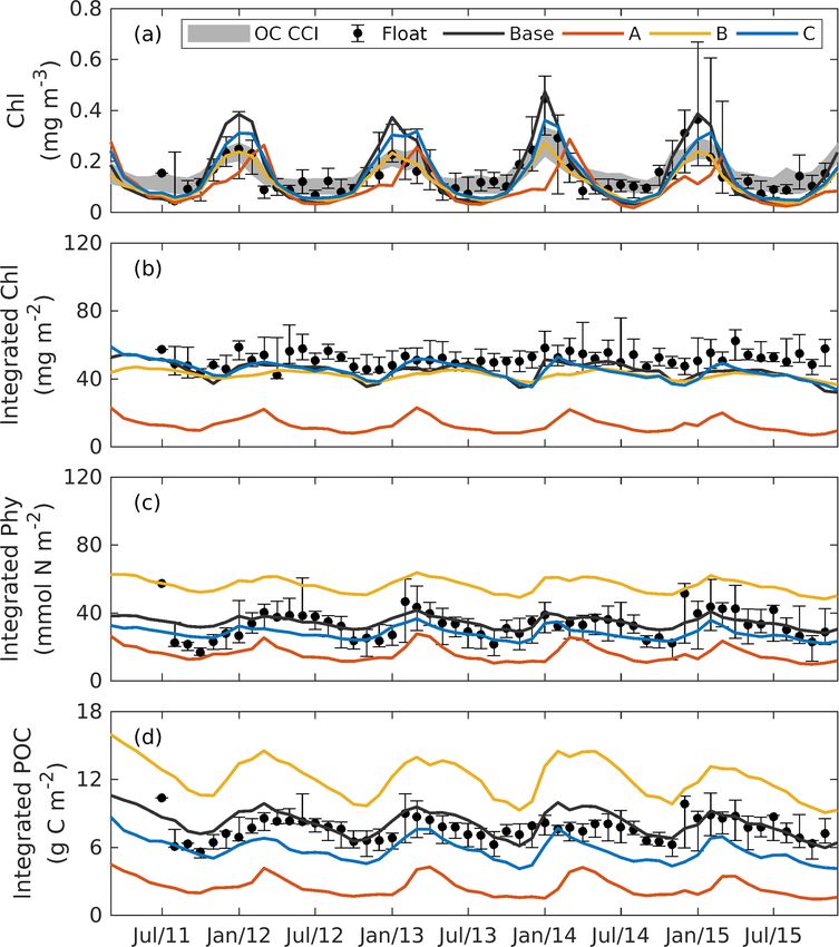
4060                       B. Wang et al.: Values of biogeochemical Argo profiles for biogeochemical model optimization

model results and available observations is minimized by it-
eratively varying parameters (Matear, 1995; Prunet et al.,
1996b, a; Fennel et al., 2011; Friedrichs et al., 2007; Kuhn
et al., 2015, 2018). However, even formal optimization typ-
ically cannot constrain all biogeochemical parameters (i.e.,
provide optimal parameter estimates with relatively small un-
certainties) because of insufficient information in the avail-
able observations (Matear, 1995; Fennel et al., 2001; Ward
et al., 2010; Bagniewski et al., 2011). For example, Matear
(1995) used a so-called simulated annealing algorithm to op-
timize three different ecosystem models and found that, even
for the simplest nutrient–phytoplankton–zooplankton model,
not all independent parameters could be constrained well,
leaving the others with large uncertainty ranges. A more re-
cent study reported that the lack of zooplankton observations
led to poor accuracy of the optimized zooplankton-related
                                                                  Figure 1. Model bathymetry (unit: m) with trajectories of six bio-
parameters when using a suite of Lagrangian-based obser-
                                                                  optical floats (small colored dots and lines) which were operated
vations during the North Atlantic spring bloom (Bagniewski        in the Gulf of Mexico from 2011 to 2015. The location of the 1D
et al., 2011). A broader suite of observation types should be     model is denoted by the large orange dot. The north and south black
favorable to parameter optimization although complications        boxes represent the Mississippi Delta and the central gulf, respec-
can arise. For example, when optimizing a suite of 1D mod-        tively, to show comparisons of surface chlorophyll in Fig. S5.
els for the Mid-Atlantic Bight, the use of satellite particu-
late organic carbon (POC) observations in addition to satel-
lite chlorophyll did not yield further improvements in model–     several biological and chemical properties throughout the up-
data fit but degraded the representation of chlorophyll (Xiao     per ocean with high resolution, over broad spatial scales and
and Friedrichs, 2014a).                                           for sustained periods (Roemmich et al., 2019). In particular,
   Typically surface ocean chlorophyll from satellite is the      the biogeochemical (BGC) Argo program (Roemmich et al.,
main source of observations for model validation (e.g.,           2019; Group, 2016) will provide temporally evolving 3D in-
Doney et al., 2009; Gomez et al., 2018; Lehmann et al.,           formation on biogeochemical variability at previously unob-
2009) and parameter optimization (Prunet et al., 1996b; Xiao      served scales. Here we assess to what degree observations of
and Friedrichs, 2014a, b), supplemented by other observa-         chlorophyll fluorescence and particle backscatter from Argo
tion types as available. However, satellites only see the ocean   profiles improve the prospects of optimizing a biogeochemi-
surface and do not resolve the vertical distribution of chloro-   cal model for the Gulf of Mexico.
phyll. This is especially problematic in oligotrophic regions        Since the high computational cost and storage demands of
where the deep chlorophyll maximum (DCM) is relatively            3D models make direct application of most parameter opti-
deep and hardly observed by the satellite (Cullen, 2015;          mization techniques difficult (but see Mattern et al., 2012;
Fennel and Boss, 2003). In addition, although chlorophyll         Mattern and Edwards, 2017; Tjiputra et al., 2007, for excep-
has long been used as a proxy of phytoplankton biomass            tions), they are typically applied in computationally efficient
and to estimate primary production based on some assump-          1D models before using the resulting parameters in the 3D
tions (Behrenfeld and Falkowski, 1997), it is not a direct        version (e.g., Hoshiba et al., 2018; Kane et al., 2011; Kuhn
measure of carbon-based phytoplankton biomass. The ra-            and Fennel, 2019; Schartau and Oschlies, 2003). We follow
tio of chlorophyll-to-phytoplankton carbon varies by at least     the latter approach here.
an order of magnitude due to physiological responses of              The main objective of this study is to assess the added
phytoplankton to their ambient environment (e.g., nutrients,      value of bio-optical profile information from Argo floats for
light, and temperature) (Cullen, 2015; Fennel and Boss,           biogeochemical model optimization in the Gulf of Mexico.
2003; Geider, 1987). Changes in chlorophyll may result from       We first examine the feasibility of improving the 3D model
physiologically induced modifications of the chlorophyll-         by applying the optimal parameters from 1D model optimiza-
to-phytoplankton ratio rather than actual changes in phyto-       tions with some minor manual modifications. We find that
plankton biomass (Pasqueron de Fommervault et al., 2017;          the gains from the 1D optimizations transfer to the 3D ver-
Mignot et al., 2014). Satellite surface chlorophyll alone is      sion. Then, by using different combinations of satellite and
therefore likely insufficient for model validation and for con-   float observations, we show that parameters optimized with
straining biogeochemical models via parameter optimiza-           respect to satellite data cannot reproduce subsurface distri-
tion.                                                             butions unless the float observations (i.e., chlorophyll, phy-
   Recent advances in autonomous platforms and sensors            toplankton, and POC) are also used.
have opened opportunities for simultaneous measurement of

Biogeosciences, 17, 4059–4074, 2020                                                   https://doi.org/10.5194/bg-17-4059-2020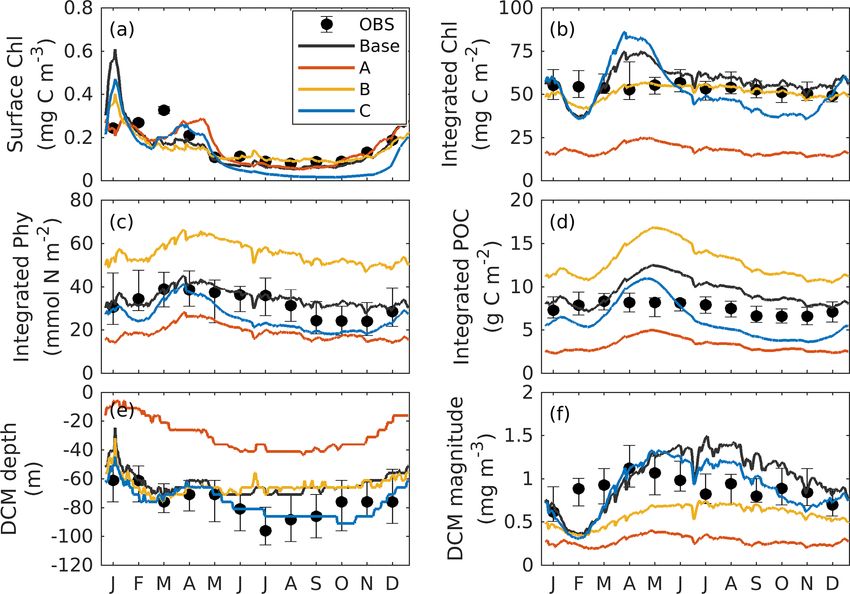
B. Wang et al.: Values of biogeochemical Argo profiles for biogeochemical model optimization                                 4061

2     Study region                                                 While the surface chlorophyll measurements from the floats
                                                                   and the satellite estimates both showed a typical seasonal cy-
The Gulf of Mexico (GOM) is a semienclosed marginal sea            cle and were highly correlated (R 2 = 0.74; see Figs. S1 and
(Fig. 1) which is characterized by eutrophic coastal waters        S2a in the Supplement), the satellite underestimated the float-
on the northern shelf and an oligotrophic deep ocean. The          measured chlorophyll concentrations in winter (Fig. S1c).
high productivity in the northern coastal region is fueled by      Satellite estimates were therefore corrected following the re-
large nutrient and freshwater inputs from the Mississippi and      gression equation shown in Fig. S2a.
Atchafalaya rivers. The large nutrient load and strong strat-         The backscatter sensor carried by the floats provided the
ification driven by Mississippi and Atchafalaya River inputs       volume scattering function at a centroid angle of 140◦ and a
lead to summer hypoxia and ocean acidification in bottom           wavelength of 700 nm (β(140◦ , 700 nm) m−1 sr−1 ). The pro-
waters on the northern shelf (Laurent et al., 2017; Yu et al.,     files were filtered (Briggs et al., 2011) to remove spikes and
2015), but nutrient export across the shelf break into the open    then converted into bbp700 following Green et al. (2014).
gulf is minor (Xue et al., 2013).                                  After that, profiles of bbp700 were converted into bbp470
   The deep ocean of the GOM is oligotrophic. Previous             based on a power law (Boss and Haëntjens, 2016) to obtain
satellite-based studies have revealed a clear seasonal cycle in    the phytoplankton (mmol N m−3 ) and POC (mg C m−3 ) esti-
surface chlorophyll, with the highest concentrations in win-       mates:
ter and the lowest in summer (Martínez-López and Zavala-                         λ1 −γ
Hidalgo, 2009; Muller-Karger et al., 1991, 2015). Thanks to        bbp(λ1) =             bbp(λ2),                              (1)
advances in autonomous profiling technology, recent studies                       λ2
based on simultaneous measurements of subsurface chloro-                              bbp470 − 76 × 10−5
                                                                   Phy = 30 100 ×                          ,                   (2)
phyll and backscatter have demonstrated that the seasonal                                 12 × 6.625
variability of surface chlorophyll might be a result of the ver-   log 10(POC) = 1.22 × log 10(bbp470) + 5.15,                 (3)
tical redistribution of subsurface chlorophyll and/or physi-
ological response to solar radiation of phytoplankton (Pas-        where λ1 and λ2 represented the measured wavelength, and
queron de Fommervault et al., 2017; Green et al., 2014).           γ was estimated as 0.78 based on the global measurements.
                                                                   The relationships for phytoplankton (Martinez-Vicente et al.,
                                                                   2013, Eq. 2) and POC (Rasse et al., 2017, Eq. 3) were ob-
3     Methods                                                      tained from a dataset for the Atlantic Ocean that covered a
                                                                   wide range of oceanographic regimes from eutrophic to olig-
3.1    Biological observations                                     otrophic ecosystems. The scale factors of 12 and 6.625 in
                                                                   Eq. (2) represented the molecular weight of carbon and the
Monthly averaged satellite chlorophyll from the Ocean              Redfield ratio to convert phytoplankton concentrations from
Colour Climate Change Initiative project (OC-CCI, http:            mg C m−3 to mmol N m−3 . The intercept 76×10−5 in Eq. (2)
//www.oceancolour.com/, last access: 25 April 2017) with           represented the background backscatter of nonalgal detritus,
a spatial resolution of 4 km from 2010 to 2015 was used            which based on Behrenfeld et al. (2005) was the backscat-
for model validation and parameter optimization. These data        ter value when chlorophyll was zero. However, in this study,
were provided by the European Space Agency (ESA), which            the majority (87 %) of bbp470 in the upper 200 m was below
produced a set of validated and error-characterized global         the intercept, and the resulting phytoplankton concentrations
ocean color products by merging SeaWiFS (Sea-viewing               were therefore close to zero, which is unrealistic in the Gulf
Wide Field-of-view Sensor), MODIS (Moderate Resolution             of Mexico. Therefore, the satellite estimate of bbp670 from
Imaging Spectroradiometer), MERIS (Medium Resolution               OC-CCI was converted into bbp700 and compared with the
Imaging Spectrometer), and VIIRS (Visible Infrared Imag-           float measurements. Compared to surface chlorophyll, sur-
ing Radiometer Suite) products.                                    face bbp700 has a less distinct seasonal cycle (Fig. S3). For
   In addition to the satellite-based measurements, bio-           example, the coefficient of variation, defined as the ratio be-
optical measurements from six autonomous profiling floats          tween standard deviation and mean to show the extent of
were used (Fig. 1), which were deployed by the Bureau of           variability, is much lower for bbp700 (0.09 and 0.07 for floats
Ocean Energy Management (BOEM) and operated in the                 and satellite, respectively) than for chlorophyll (0.31 and
deep GOM from 2011 to 2015. These floats were equipped             0.26 for floats and satellite, respectively). The float bbp700
with a CTD and bio-optical sensors to collect biweekly pro-        is weakly correlated with the satellite estimates (R 2 = 0.11)
files of temperature, salinity, chlorophyll, and backscatter at    and generally lower by a factor of ∼ 0.45 than the satellite es-
700 nm (bbp700 (m−1 )) from the surface to 1000 m depth            timates (Fig. S2b). The bbp700 profiles were therefore mul-
(see Pasqueron de Fommervault et al., 2017; Green et al.,          tiplied by 2.2 before being converted to bbp470. As a result,
2014, for more details). Chlorophyll was derived from fluo-        the mean value of the bbp470 (88×10−5 m−1 ) is close to the
rescence based on the sensor manufacturer’s calibrations and       intercept in Eq. (2) when chlorophyll went to zero. Further-
compared with the satellite estimates of surface chlorophyll.      more, the resulting concentrations of phytoplankton biomass

https://doi.org/10.5194/bg-17-4059-2020                                                   Biogeosciences, 17, 4059–4074, 2020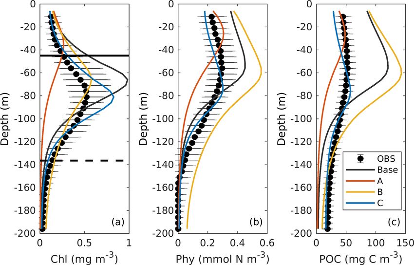
4062                            B. Wang et al.: Values of biogeochemical Argo profiles for biogeochemical model optimization

Table 1. Initial values and ranges of biogeochemical model parameters.

                   Descriptions (unit)                                                          Symbol     Value     Range
                   Radiation threshold for nitrification (W m−2 )                               I0         0.0095a   0.005b –0.01b
                   Half-saturation radiation for nitrification (W m−2 )                         kI         0.1a      0.01b –0.5b
                   Maximum nitrification rate (d−1 )                                            nmax       0.2c      0.01b –0.35b
                   Phytoplankton growth at 0 ◦ C (dimensionless)                                µ0         0.69a     0.1b –3.0b
                   Initial slope of P -I curve (mg C (mg Chl W m−2 d)−1 )                       α          0.125a    0.007a –0.13a
                   Half saturation for NO3 uptake (mmol N m−3 )                                 kNO3       0.5a      0.007a –1.5a
                   Half saturation for NH4 uptake (mmol N m−3 )                                 kNH4       0.5a      0.007a –1.5a
                   Phytoplankton mortality (d−1 )                                               mp         0.075     0.01b –0.2b
                   Aggregation parameter (d−1 )                                                 τ          0.1       0.01b –25b
                   Maximum chlorophyll-to-carbon ratio (mg Chl mg C−1 )                         θmax       0.0535c   0.005a –0.15b
                   Phytoplankton sinking velocity (m d−1 )                                      wPhy       0.1a      0.009a –25a
                   Maximum grazing rate (d−1 )                                                  gmax       0.6a      0.1b –4b
                   Half saturation for phytoplankton ingestion ((mmol N m−3 )2 )                kp         0.5       0.01b –3.5a
                   Zooplankton assimilation efficiency (dimensionless)                          β          0.75a     0.25b –0.75b
                   Zooplankton basal metabolism (d−1 )                                          lBM        0.01      0.01b –0.15b
                   Zooplankton specific excretion (d−1 )                                        lE         0.1a      0.05b –0.35b
                   Zooplankton mortality (d−1 )                                                 mZ         0.2       0.02b –0.35b
                   Small detritus remineralization (d−1 )                                       rSD        0.3c      0.005b –0.25a
                   Large detritus remineralization (d−1 )                                       rLD        0.1       0.005b –0.25a
                   Small detritus sinking velocity (m d−1 )                                     wSDet      0.1a      0.009a –25a
                   Large detritus sinking velocity (m d−1 )                                     wLDet      1a        0.009a –25a
                 a Fennel et al. (2006). b Kuhn et al. (2018). c Yu et al. (2015).

and POC as well as the ratio of chlorophyll to phytoplankton                         Forecast ERA-Interim product with a horizontal resolu-
biomass are reasonable (please see Figs. 4 and 10). This gave                        tion of 0.125◦ (ECMWF reanalysis, https://www.ecmwf.int/
us confidence in our conversion process for float backscatter                        en/forecasts/datasets/reanalysis-datasets/era-interim, last ac-
and our choice of empirical equations relating backscatter to                        cess: 17 August 2018). A bulk parameterization was applied
phytoplankton and POC.                                                               to calculate the surface net heat fluxes and wind stress. The
                                                                                     model was one-way nested inside the 1/12◦ data-assimilative
3.2    Three-dimensional model description                                           global HYCOM/NCODA (https://www.hycom.org, last ac-
                                                                                     cess: 2 November 2017). Tidal constitutes were neglected in
                                                                                     the model.
The physical model was configured based on the Regional
                                                                                        The biogeochemical model used a seven-component
Ocean Modeling System (Haidvogel et al., 2008, ROMS,
                                                                                     model (Fennel et al., 2006) to simulate the nitrogen cycle
https://www.myroms.org, last access: 16 June 2016) for the
                                                                                     in the water column. The model described the dynamics of
Gulf of Mexico (Fig. 1). The model has a horizontal res-
                                                                                     two species of dissolved inorganic nitrogen (nitrate, NO3 ,
olution of ∼ 5 km and 36 terrain-following sigma layers
                                                                                     and ammonium, NH4 ), one function of phytoplankton (Phy),
with refined resolution near the surface and bottom as in
                                                                                     chlorophyll (Chl) as a separate state variable which allowed
Yu et al. (2019). The model solved the horizontal and ver-
                                                                                     photo-acclimation based on the model of Geider et al. (1997),
tical advection of tracers using the multidimensional pos-
                                                                                     one function of zooplankton (Zoo), and two pools of detritus
itive definitive advection transport algorithm (MPDATA,
                                                                                     (i.e., small suspended detritus, SDeN, and large fast-sinking
Smolarkiewicz and Margolin, 1998). Horizontal viscosity
                                                                                     detritus, LDeN). Water–sediment interactions were simpli-
and diffusivity were parameterized by a Smagorinsky-type
                                                                                     fied by an instantaneous remineralization parameterization,
formula (Smagorinsky, 1963), and vertical turbulent mix-
                                                                                     where detritus sinking out of the water column immediately
ing was calculated by the Mellor–Yamada 2.5-level closure
                                                                                     resulted in a corresponding influx of ammonium into the bot-
scheme (Mellor and Yamada, 1982). Bottom friction was
                                                                                     tom layer. Detailed descriptions of the model equations can
specified by a logarithmic drag formulation with a bottom
                                                                                     be found in Fennel et al. (2006) and Laurent et al. (2017).
roughness of 0.02 m. The model was forced by 3-hourly
                                                                                     The biological model parameters are listed in Table 1.
surface heat and freshwater fluxes; 6-hourly air tempera-
                                                                                        The model received freshwater, nutrients (NO3 and NH4 ),
ture, sea level pressure, and relative humidity; and 10 m
                                                                                     and organic matter inputs from major rivers along the Gulf
winds from the European Centre for Medium-Range Weather

Biogeosciences, 17, 4059–4074, 2020                                                                      https://doi.org/10.5194/bg-17-4059-2020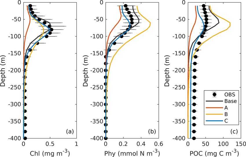
B. Wang et al.: Values of biogeochemical Argo profiles for biogeochemical model optimization                                 4063

Coast. Freshwater and nutrients from the Mississippi and           ature was 5 ◦ C lower than at the surface, and was obtained
Atchafalaya rivers were prescribed based on the daily mea-         from daily outputs of the 3D model. The model was inte-
surements by the US Geological Survey river gauges. River          grated in time using the Crank–Nicolson scheme for vertical
particulate organic nitrogen (PON) was assigned to the small       turbulent mixing and an implicit time-stepping scheme for
detritus pool and determined as the difference between to-         the biogeochemical tracers, which were treated identically
tal Kjeldahl nitrogen and ammonium (Fennel et al., 2011).          to the 3D model. Some of the biogeochemical parameteriza-
Other rivers utilized the climatological estimates of freshwa-     tions required input of temperature and solar radiation, which
ter, nutrients, and PON as in Xue et al. (2013).                   were also taken from the 3D model. As the 1D model did
   Initial and open boundary conditions for NO3 were speci-        not consider horizontal and vertical advection, NO3 below
fied by applying an empirical relationship between NO3 and         100 m was nudged to that from the 3D base simulation with
temperature, derived from the World Ocean Atlas (WOA;              a nudging timescale of 20 d. The 1D model was run for the
Fig. S4a), that was applied to the temperature fields from         year 2010 repeatedly for three cycles, with the first two being
HYCOM/NCODA. Analogously, empirical relationships be-              model spin-up and the last annual cycle used to calculate the
tween chlorophyll and density (Fig. S4b), phytoplankton and        misfit between the model and observations.
density (Fig. S4c), and POC and density (Fig. S4d) were
obtained from the median profiles of the bio-optical floats        3.4   Parameter optimization method
and used to derive initial and boundary conditions for these
variables. Zooplankton and small detritus were assumed to          The evolutionary algorithm described by Kuhn et al. (2015,
amount to 10 % of phytoplankton biomass and the remaining          2018) was used to search for optimal model parameters by
fractions of POC attributed to large detritus. Sensitivity tests   minimizing the misfit between the model and observations.
showed that changing these allocations had little impact on        The misfit was measured by the following cost function:
our model results.                                                        V
                                                                   F (−
                                                                      →     Fv −
                                                                               →
                                                                          X
   A 6-year (5 January 2010–31 December 2015) hindcast                p)=      p ,                                             (4)
was performed that included the period of operation of the                   v=1
bio-optical floats. The first year was considered model spin-                         Nv
                                                                               1 X
                                                                   Fv −
                                                                      →                  ŷi,v − yi,v −
                                                                                                      →
                                                                                                       2
up and the next 5 years are discussed.                                p =                             p ,                      (5)
                                                                              Nv σv2 i=1

3.3   One-dimensional model description                            where − →p represented the parameters vector, V was the num-
                                                                   ber of different observation types, Nv was the number of ob-
As optimizing a 3D biogeochemical model is computation-            servations for each variable, and Fv (−  →p ) was the misfit for
ally expensive, it was more practical to perform the opti-         observation type v measured as the mean-square difference
mization using a reduced-order model surrogate. A surro-           between observations (ŷ) and corresponding model estimates
gate can be a coarser-resolution model, a simplified model,        (y(−→p )). The cost function Fv (− →p ) was normalized by the
or a reduced-dimension model. In this study, a 1D model            standard deviation of each variable type (σv ) in order to re-
was used to optimize the biological parameters of the 3D           move the effect of different units.
model. This approach has been successfully used previously             The algorithm is inspired by the rules of natural selection.
(Hoshiba et al., 2018; Kane et al., 2011; Oschlies and Schar-      Following Kuhn et al. (2015), an initial parameter popula-
tau, 2005).                                                        tion of 30 parameter vectors was randomly generated within
   The 1D model, which is similar to that used by Lagman           a predefined range of parameters (see Table 1). The model
et al. (2014) and Kuhn et al. (2015), covered the upper 200 m      was evaluated for each parameter vector and the resulting
of the ocean with a vertical resolution of 5 m and was con-        cost function was calculated. For this initial generation and
figured at one location in the open gulf (see Fig. 1). This        each of the following generations, the half of the population
relatively fine vertical resolution was used because it was        with the lower misfit survived into the next generation. The
close to that of our BGC-Argo floats (4–6 m in upper 200 m)        other half was regenerated through a recombination of sur-
and was much higher than the 3D model whose vertical res-          vivors in a process analogous to genetic crossover. In addi-
olution varies from a few meters near the surface to about         tion, each newly generated population was subject to ran-
50 m near at 200 m depth around the 1D station. In the verti-      dom mutations by multiplying the parameter values by a ran-
cal direction, the water column was divided into two layers:       dom value between 0 and 2. Parameter values exceeding the
the turbulent surface layer and a quiescent layer below. A         predefined range were replaced by their corresponding min-
higher diffusion coefficient (KZ1 = max(HMLD 2    /400, 10), in    imum or maximum limits to avoid unrealistic values. The
           2  −1
unit of m d ) was applied in the turbulent surface layer,          above procedure was performed iteratively for 300 genera-
and a lower diffusion coefficient (KZ2 = KZ1 /2) was as-           tions to reach the minimum of the cost function, which cor-
signed to the quiescent bottom layer. The interface between        responded to the optimal parameter set.
these two layers was determined by the mixed layer depth               Previous parameter optimization studies have shown that
(HMLD , in unit of m), defined as the depth where the temper-      it is difficult to constrain all model parameters even for very

https://doi.org/10.5194/bg-17-4059-2020                                                   Biogeosciences, 17, 4059–4074, 2020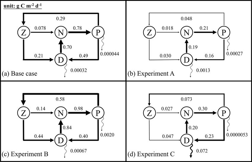
4064                         B. Wang et al.: Values of biogeochemical Argo profiles for biogeochemical model optimization

                                                                       from the BGC-Argo floats were used. For the climatologi-
                                                                       cal profiles, all float profiles in the gulf were averaged be-
                                                                       cause the deep Gulf of Mexico is homogenous horizontally
                                                                       and only few profiles were available in the immediate vicin-
                                                                       ity of the 1D station.
                                                                          To assess the effects of the optimization with respect to
                                                                       the different observation types, we conducted three groups of
                                                                       experiments in which (A) surface satellite chlorophyll only,
                                                                       (B) surface satellite chlorophyll and float profiles of chloro-
                                                                       phyll, and (C) surface satellite chlorophyll and float profiles
                                                                       of chlorophyll, phytoplankton, and POC were used. For each
                                                                       of these three groups, four to five optimizations were con-
                                                                       ducted, starting with the three most sensitive parameters and
                                                                       then adding one more parameter at a time (Table 2) guided
                                                                       by the sensitivity analysis with respect to the observed vari-
                                                                       ables they used. Specifically, groups A and B were based
Figure 2. Parameter sensitivities (unit: dimensionless) with respect   on the sensitivity analysis with respect to chlorophyll, while
to (a) chlorophyll and (b) the sum of chlorophyll, phytoplankton,      group C was based on the sensitivity analysis with respect to
and POC.                                                               the sum of chlorophyll, phytoplankton, and POC. Each op-
                                                                       timization was replicated four times. The optimization with
                                                                       the smallest model–data misfit within each group was then
simple ecosystem models because the information content of             used. Prior tests have shown that the available observations
available observations is typically insufficient (Matear, 1995;        cannot simultaneously constrain the sinking rates of small
Fennel et al., 2001; Ward et al., 2010). Here we conducted             and large detritus (wSDet and wLDet ) because an increase in
sensitivity tests to identify the parameters that were most sen-       one parameter can be counteracted by a decrease in the other.
sitive to the available observations and chose a subset of these       Therefore, a constant ratio of 0.1 between these two parame-
to be optimized. In the base case, all parameters were at their        ters (wSDet = 0.1 × wLDet ) was imposed based on their prior
initial guess values obtained from the previous literature and         values, and only one of the two was optimized. In groups
some initial tuning (Table 1). Then the test cases were run            A and B, the aggregation parameter τ was fixed at 0.05 be-
multiple times by incrementally changing one parameter at              cause prior tests generated unreasonably high values for this
a time to be the minimum; the first, second, and third quar-           parameter.
tile; and the maximum of its corresponding range while set-               We report two different metrics of misfits for these groups
ting the other parameters to their initial guess value (Table 1).      of experiments. The first metric, which we refer to as the
The sensitivity was measured as the sum of a normalized ab-            case-specific cost function value, is based on the optimized
solute difference between the base case (yBase ) and the test          observations in a given experiment and was minimized by
case (yTest ):                                                         the optimization algorithm, i.e.,

        1X m      n
               1X     |yBase − yTest |
Q y, −
     →
                                                                       FA −
                                                                          →
                                                                          p = FsurfCHL −→

     p =                               ,                        (6)                     p ,                                       (7)
         m i=1 n j =1     yBase
                                                                       FB −
                                                                          →
                                                                          p = FsurfCHL −→
                                                                                        p + FChl −→

                                                                                                   p ,                            (8)
                                                                       FC −
                                                                          →
                                                                          p =FsurfCHL − →
                                                                                        p + FChl −
                                                                                                 →

where m is the number of parameter increments (here 5) and                                        p + ...
n is the number of base–test pairs consisting of all 1D model                 F     −
                                                                                    →
                                                                                    p +F      −
                                                                                              →
                                                                                               p .                                (9)
                                                                                   Phy          POC
grid cells throughout the whole simulation period for all vari-
ables to be compared.
   Results of the sensitivity analysis are shown in Fig. 2,               However, the models with lower case-specific misfit do not
where parameters are ranked by sensitivity with respect to             necessarily have better predictive skill in reproducing the un-
chlorophyll (Fig. 2a) and the sum of chlorophyll, phytoplank-          optimized observations because of the so-called overfitting
ton, and POC (Fig. 2b). POC is the sum of phytoplankton,               problem; e.g., the model might be tuned to reproduce opti-
zooplankton, and small and large detritus.                             mized observations through wrong mechanisms (Friedrichs
                                                                       et al., 2006). To account for this, a second metric referred to
3.5    Parameter optimization experiments                              as the total misfit is given by Eq. (9). For group C, the sec-
                                                                       ond metric is the same as the case-specific cost function. For
For the parameter optimization of the 1D model, satellite              groups A and B, the total misfit metric allows us to assess
chlorophyll within a 3 pixel × 3 pixel (12 km × 12 km) area            improvements in the model’s predictive skill to represent un-
around the 1D station and monthly climatological profiles              optimized fields.

Biogeosciences, 17, 4059–4074, 2020                                                      https://doi.org/10.5194/bg-17-4059-2020
B. Wang et al.: Values of biogeochemical Argo profiles for biogeochemical model optimization 4065
Table 2. The best fit of parameter set for each optimization experiment. Dashed lines represent that these parameters are not included in the
parameter optimization and use their prior values. The optimal optimization A4, B2, and C4 which are further discussed and are denoted
simply as experiment A, B, and C are highlighted as bold.
wPhy mP kNH4 τ θmax α wLDet
Base 0.1000 0.0750 0.5000 0.1000 0.0535 0.1250 1.000
A1 0.0608 0.0100 1.5000 – – – –
1D model A2 0.6863 0.0100 0.0195 – 0.0169 – –
A3 1.6567 0.1978 0.1004 – 0.0250 0.0219 –
A4 0.9468 0.0737 0.2454 – 0.0191 0.0101 4.9694
3D model A 0.9468 0.0737 0.0100 – 0.0191 0.0101 4.9694
B1 0.2863 0.0983 1.5000 – – – –
B2 0.4217 0.0130 0.0300 – 0.0158 – –
1D model
B3 2.1016 0.0176 1.5000 – 0.0346 0.0079 –
B4 0.0009 0.0100 1.5000 – 0.0361 0.0405 8.3514
3D model B 0.4217 0.0130 0.0100 – 0.0158 – –
wPhy rLD mP τ kNH4 wLDet θmax
Base 0.1000 0.1000 0.0750 0.1000 0.5000 1.0000 0.0535
C1 1.9231 0.2500 0.1805 – – – –
C2 0.9755 0.2500 0.0100 1.1402 – – –
1D model
C3 0.4071 0.0630 0.0100 1.8531 0.0070 – –
C4 0.0090 0.0050 0.0634 0.0995 0.0431 5.6623 –
C5 0.0090 0.2245 0.0100 0.6451 1.5000 2.5202 0.0614
3D model C 0.0090 0.0050 0.0634 0.0500 0.0100 5.6623 –
4 Optimization of 1D models
4.1 Observations and base case
To provide context for the evaluation of our optimization ex-
periments, the observations and the base case will be de-
scribed first. As shown in Fig. 3a, the observed surface
chlorophyll shows a clear seasonality with the high concen-
trations in winter and low concentrations in summer. In the
base case, the simulated surface chlorophyll fits observations
well. Unlike the surface chlorophyll, the observed integrated
chlorophyll as well as the phytoplankton and POC over the
upper 200 m tend to be more constant with much less sea-
sonality (Fig. 3b–d). This has been reported by Pasqueron
de Fommervault et al. (2017), who attributed the seasonality
Figure 3. Annual cycle of surface chlorophyll (a), vertically inte- of surface chlorophyll to the vertical redistributions of sub-
grated chlorophyll (b), vertically integrated phytoplankton (c), ver- surface chlorophyll and/or photoacclimation rather than real
tically integrated POC (d), and the depth (e) and magnitude (a) changes in biomass.
of the DCM from observations (black dots with error bars); the The DCM is a ubiquitous phenomenon in the oligotrophic
base case (black lines); and experiment A (orange lines; only satel- regions and can form independently of the biomass maxi-
lite surface chlorophyll is used), B (yellow lines; satellite surface mum (Cullen, 2015; Fennel and Boss, 2003). In this study,
chlorophyll and float profiles of chlorophyll are used), and C (blue
we define the DCM depth as where the maximum of subsur-
lines; all available observations are used). Chlorophyll, phytoplank-
ton, and POC are integrated over the top 200 m. Black error bars
face chlorophyll is. Observations detect a predominant DCM
represent the interquartile range of observations. at around 60–100 m depth throughout the whole year, with
a sharp deepening in June and gradual shoaling after July
(Fig. 3e), reflecting the seasonality of the solar radiation. Un-
like the large variability in the depth of the DCM, its magni-
https://doi.org/10.5194/bg-17-4059-2020 Biogeosciences, 17, 4059–4074, 20204066 B. Wang et al.: Values of biogeochemical Argo profiles for biogeochemical model optimization
4.2 Results of the optimizations
4.2.1 Model–data misfits
The case-specific cost function values and total misfits for
the different 1D optimizations are shown in Fig. 5. Not sur-
prisingly, all optimizations result in a reduction of the case-
specific cost function values. The extent of the reductions
depends on the specific subset of parameters that were op-
timized. However, the total misfits are not reduced in all op-
timizations. Optimizations A1 and A2 lead to slightly larger
total misfits than the base case, and optimization B2 leads to
a significantly larger total misfit. The smallest total cost func-
tion values are achieved in A4, B4, and C4, i.e., in the exper-
Figure 4. Observed (black dots with error bars) and simulated (col- iments where a larger subset of parameters was optimized
ored lines) vertical profiles of chlorophyll, phytoplankton, and POC. (six parameters). The optimal parameter sets (A4, B2, and
Black errors represent the interquartile range of observations. The C4), which are selected based on case-specific misfit from
solid and dashed black lines in (a) represent the median values of these three groups, will be used in subsequent analyses and
mixed layer depth from July and December.
hereafter are denoted simply as experiment A, experiment B,
and experiment C. Further comparisons are presented below
tude is relatively constant at around 0.62 mg m−3 (Fig. 3f). In to assess the impact of the different combinations of obser-
the annually averaged profiles, the observed DCM is located vations.
at about 80 m depth with a concentration of 0.52 mg m−3
(Fig. 4a). The base case succeeds in reproducing the DCM 4.2.2 Experiment A: satellite chlorophyll only
at 65 ± 7 m depth. However, it fails to reproduce the deep-
ening of the DCM in June, and the simulated annually av- The optimal parameters (Table 2) from experiment A yield a
eraged depth of DCM is shallower by about 15 m than the 58 % reduction in the misfit for surface chlorophyll (Fig. 5d).
observed. The simulated magnitude of the DCM is about 2- However, the vertical structure of chlorophyll deteriorates
fold larger than the observed (Figs. 3f and 4a), and hence relative to the base case (Fig. 4a) because of inappropriate es-
the base case generally overestimates vertically integrated timates of the initial slope (α = 0.0101; see Table 2) and the
chlorophyll (Fig. 3b). maximum ratio of chlorophyll to carbon (θmax = 0.0191; see
With respect to phytoplankton and POC, the observed Table 2). The annually averaged depth of the DCM is lifted
maximum concentration occurs at about 60 m depth, which is up to around 30 ± 10 m, and the magnitude of DCM strongly
20 m above the DCM (Fig. 4b–c). The observed vertical dis- decreases (Figs. 3a, 4b). Similar to chlorophyll, these deteri-
tributions of phytoplankton and POC are not well captured orations also manifest in the vertical phytoplankton and POC
by the base case. For example, phytoplankton and POC in the distributions (Fig. 4b–c). As a result, experiment A underes-
upper layer are overestimated with the model–data discrep- timates vertically integrated chlorophyll, phytoplankton, and
ancies exceeding the variability of the observations (Fig. 4b– POC (Fig. 3b–d).
c). As a result, the base case yields an overall overestimation
of the vertically integrated phytoplankton and POC (Fig. 3c– 4.2.3 Experiment B: satellite chlorophyll and
d). chlorophyll profiles
Figure 4b also shows that both observed and simulated
phytoplankton approach zero at about 160 m depth. Unlike Due to the addition of observed chlorophyll profiles to the
phytoplankton, the observations show that the POC concen- optimization in experiment B, the misfits for surface and
trations are 19 mg C m−3 at about 200 m depth because of subsurface chlorophyll decrease relative to the base case
the existence of detritus, or zooplankton, or both (Fig. 4b, c). (Fig. 5d), but the reduction in the misfit for surface chloro-
However, the base case fails to reproduce these nonzero POC phyll (38 %) is smaller than that in experiment A (58 %).
concentrations, indicating that the model might be underesti- A straightforward interpretation is that the addition of sub-
mating the carbon export fluxes at 200 m. surface observations reduces the model’s degrees of freedom
to fit one single observation type (surface chlorophyll). The
vertical profile of chlorophyll is reproduced better in exper-
iment B than in the base case and experiment A in that the
magnitude of the DCM is closer to the observations, although
the DCM depth is still too shallow, on average by about 20 m
(Fig. 4a). The improvement in the vertical chlorophyll struc-
Biogeosciences, 17, 4059–4074, 2020 https://doi.org/10.5194/bg-17-4059-2020B. Wang et al.: Values of biogeochemical Argo profiles for biogeochemical model optimization 4067
4.3 Simulated carbon fluxes
Annually averaged carbon fluxes within the upper 200 m are
shown for each experiment in Fig. 6. The primary produc-
tion in the base case amounts to 0.78 g C m−2 d−1 , of which
37 % is consumed by zooplankton, and the remaining 63 %
flows into detritus pools through sloppy feeding, mortality,
and aggregation of phytoplankton. As for the production of
detritus, contributions from the phytoplankton and zooplank-
ton pools account for 70 % and 30 %, respectively. Most of
the produced detritus is recycled into the nutrient pool fu-
eling recycled primary production, and only a small frac-
tion is removed from the upper layer through gravitational
Figure 5. The case-specific cost function values (a–c) and total mis- sinking. As a result, carbon export, which is estimated as
fits (d) of the base case and the different optimizations. the sum of sinking fluxes by phytoplankton and detritus, is
only 0.00032 g C m−2 d−1 and accounts for 0.04 % of pri-
mary production.
ture results in a better model–data fit of vertically integrated Due to the underestimation of phytoplankton in experi-
chlorophyll (Fig. 3b). ment A, primary production is reduced to 0.21 g C m−2 d−1
Despite the improvements in chlorophyll, the vertical pro- in that case. All other fluxes in the top 200 m decrease rela-
files of phytoplankton and POC exhibit a marked deteriora- tive to the base case as well, except for the export flux which
tion relative to the base case and experiment A (Fig. 4b–c) increases to about 0.8 % of primary production. This rela-
because the parameter optimization underestimates the max- tive increase in export is the result of larger sinking rates of
imum chlorophyll-to-carbon ratio (θmax = 0.0158; see Ta- phytoplankton and detritus (wPhy = 0.95, wLDet = 4.97; see
ble 2). Experiment B leads to an overestimation of phy- Table 2) than those used in the base case.
toplankton and POC relative to the base case with misfits In contrast to experiment A, experiment B yields an in-
roughly 2.7 and 1.6 times larger than those of the base case, crease in primary production relative to the base case. The
respectively (Fig. 5d). Although experiment B reproduces the proportion of the grazing flux to primary production and
non-zero POC concentrations at about 200 m depth, the pro- the contribution of zooplankton to the production of detritus
portion of phytoplankton in the POC pool is incorrect. In also increase to about 59 % and 52 %, respectively. Unlike in
contrast to the observations where the phytoplankton’s con- the other three experiments, carbon export in experiment B
tribution is negligible (Fig. 4), the simulated POC at 200 m is is dominated by the sinking of phytoplankton, reflecting its
dominated by phytoplankton (49 %). large contribution to POC at 200 m. Although the simulated
POC concentration at 200 m is very close to the observations,
4.2.4 Experiment C: all available observations the relative contributions of phytoplankton, zooplankton, and
detritus are problematic and likely do not result in a better
Incorporating all observations (i.e., surface chlorophyll and
estimation of carbon export (in this case 0.3 % of primary
profiles of chlorophyll, phytoplankton, and POC) in exper-
production).
iment C improves the model–data misfits for almost all as-
In experiment C, primary production is 0.30 g C m−2 d−1 ,
pects except for surface chlorophyll (Fig. 3). Although a
with 24% flowing to zooplankton. The mortality of zoo-
slight increase in the misfit occurs for the surface chloro-
plankton causes a flux of 0.047 g C m−2 d−1 to detritus,
phyll (∼ 5 %), the total misfit is reduced by 75 % compared
which accounts for 17 % of the production of detritus. Fi-
to the base case. As shown in Fig. 4a, the annually averaged
nally, about 24 % of primary production is removed from the
depth of DCM of 80 m coincides with the observed DCM,
upper 200 m through gravitational sinking. The simulated ex-
primarily because experiment C reproduces the deepening
port ratio of 24 % is within the wide range of reported ex-
of the DCM in summer. The magnitude of the DCM is also
port ratios, from 6 % to 43 %, at 120 m depth in the Gulf of
decreased relative to the base case but remains higher than
Mexico (see Table 3 of Hung et al., 2010). Despite the high
the observed. Phytoplankton and POC profiles exhibit only
degree of uncertainty that exists when estimating export ra-
minor deviations from the observations (Fig. 4b–c). Impor-
tios (e.g., the global mean export ratio varies from ∼ 10 %
tantly, experiment C reproduces the non-zero POC concen-
Henson et al., 2012; Lima et al., 2014; Siegel et al., 2014
trations at 200 m. In contrast to experiment B, phytoplankton
to ∼ 20 % Henson et al., 2015; Laws et al., 2000), it is ob-
in experiment C drops to zero at about 160 m and POC is
vious that only experiment C reproduced an export ratio of
dominated by detritus (85 %), which is more consistent with
a reasonable magnitude. A more detailed validation of pri-
the observations.
mary production and export fluxes will be presented in the
following sections.
https://doi.org/10.5194/bg-17-4059-2020 Biogeosciences, 17, 4059–4074, 20204068 B. Wang et al.: Values of biogeochemical Argo profiles for biogeochemical model optimization
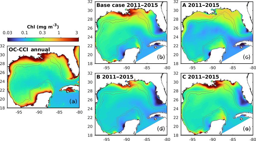
Figure 7. Spatial distributions of the annual mean chlorophyll in
the surface layer from the satellite (OC-CCI) climatology (2011–
Figure 6. Annually averaged carbon fluxes integrated over the up- 2015) and the different model versions. The gray contours mark the
per 200 m (unit: g C m−2 d−1 ) for the base case (a) and optimized bathymetric depths of 200 and 1000 m.
experiments A, B, and C. The N, P, Z, and D stand for the pools
of nutrient, phytoplankton, zooplankton, and the sum of small and
large detritus, respectively. The thickness of arrows scales with the
satellite estimates show high chlorophyll in the coastal re-
magnitude of fluxes. Dashed arrows represent fluxes lower than
0.01 g C m−2 d−1 .
gions and low chlorophyll in the deep ocean (Fig. 7a). This
spatial pattern of surface chlorophyll is well reproduced in all
simulations except in experiment A, which even fails to re-
5 Three-dimensional biogeochemical model produce the relatively high chlorophyll near the Mississippi–
Atchafalaya River systems because of the high sinking rate
The optimal parameter sets from the 1D optimizations of A, of phytoplankton (wPhy = 0.95; see Table 2). The largest
B, and C were applied in the 3D model for the whole GOM model–data differences occur in the coastal regions, where
for 5 years (2011–2015). The performance of the 3D model all simulations underestimate the observed surface chloro-
can be regarded as a cross validation of the parameters op- phyll. Since all BGC-Argo floats operated in the deep ocean
timized in 1D at different times and locations. It is possi- (Fig. 1) and the parameter optimization is performed at one
ble that the optimization algorithm has modified parameters central station without any influence from coastal environ-
to compensate for biases between 1D and 3D simulations, ments, only the model results in the deep ocean (depth >
e.g., the absence of advection in 1D model as well as the 1000 m) will be considered in the following discussion.
differences in the model domain, model period, and model
resolution, that degrade the 3D model performance (Kane 5.2 Subsurface distributions
et al., 2011). Indeed, directly applying the optimal param-
eter sets from the 1D version to the 3D model yields lower Figure 8 shows the seasonal cycles of surface chlorophyll as
model–data agreement than the 1D counterpart but preserves well as the vertically integrated chlorophyll, phytoplankton,
the most important features well. For instance, when the re- and POC within the deep ocean (depth > 1000 m). Analo-
sulting parameters were used in experiment C, chlorophyll gous to the 1D models, chlorophyll, phytoplankton, and POC
concentrations in the upper layer were lower in the 3D model were integrated over the upper 200 m. Here again the whole
and farther away from the observations. However, the DCM deep ocean was averaged because it is homogenous horizon-
depth and the non-zero POC concentrations at 200 m with tally. In addition, we compare surface chlorophyll with satel-
appropriate contributions from each component are well re- lite estimates in two subregions from the Mississippi Delta
produced in the 3D model. We therefore performed a few and the central gulf in Fig. S5.
manual tests and made the following modifications to the op- Comparisons of vertical profiles between observations and
timized parameters to bring the model–data agreement of the model results are given in Fig. 9. In general, the main features
3D model in better alignment with that of the 1D version in the 3D models are very similar to those in 1D. Experi-
(Table 2): the half saturation for NH4 uptake (kNH4 ) was de- ment A cannot constrain the vertical profiles of chlorophyll
creased to 0.01 in experiment B and C, and the aggregation because of the inappropriate estimation of initial slope (α),
parameter (τ ) was decreased to 0.05 in experiment C. experiment B overestimates phytoplankton and its contribu-
tion to POC since the maximum ratio of chlorophyll to car-
5.1 Spatial patterns of surface chlorophyll bon (θmax ) is weakly constrained, and experiment C shows
significant improvements in the model–data agreement.
First, the annual climatological surface chlorophyll from the Additional comparisons of the chlorophyll-to-carbon ra-
satellite and model are compared from 2011 to 2015. The tio, primary production, and carbon export fluxes from 1D
Biogeosciences, 17, 4059–4074, 2020 https://doi.org/10.5194/bg-17-4059-2020B. Wang et al.: Values of biogeochemical Argo profiles for biogeochemical model optimization 4069
Figure 9. Observed and simulated vertical profiles of chlorophyll,
phytoplankton, and POC from each 3D model.
tatively similar to the 1D simulations. Experiment C provides
the best estimates of PP when compared to satellite-based es-
timates from VGPM and CbPM, both in 1D and 3D.
The base case and experiments A and B yield carbon ex-
port fluxes smaller by 1 to 2 orders of magnitude than exper-
iment C. Thus, only experiment C from the 1D and 3D mod-
Figure 8. Observed and simulated seasonal cycles of surface els are shown in Fig. 10c in comparison to observations from
chlorophyll (a), vertically integrated chlorophyll (b), vertically in- sediment traps (see Supplement). The carbon export fluxes
tegrated phytoplankton (c), and vertically integrated POC (d) from at 200 m from the 1D and 3D are similar in magnitude al-
each 3D model. Solid lines represent the median values over the though the 1D model yields higher fluxes and larger variabil-
deep ocean of GOM (depth > 1000 m). Error bars and shades show ity. Despite the scarcity of carbon export observations in the
the 25 % and 75 % percentiles. Chlorophyll, phytoplankton, and GOM, the model estimates are within the range of observa-
POC are integrated over the top 200m.
tions down to ∼ 1600 m and capture the observed declining
trend of carbon export with depth.
In summary, all the results above demonstrate the feasibil-
and 3D models with observations are given in Fig. 10. The ities of using the locally optimized parameters from the 1D
chlorophyll-to-carbon ratio is estimated as the vertically in- model to improve the 3D simulation. In addition, by incor-
tegrated chlorophyll divided by phytoplankton in the up- porating all available observations (i.e., surface chlorophyll
per 200 m (Fig. 10a). As an important indicator of phyto- from satellite estimates, profiles of chlorophyll, phytoplank-
plankton physiological status (Geider, 1987), the observed ton, and POC from bio-optical floats), experiment C cannot
chlorophyll-to-carbon ratio varies considerably in response only simulate the biogeochemical processes well in the up-
to the ambient environment. In general, the ratios derived per 200 m, but also reproduce the carbon export flux and its
from the 3D models are lower than their corresponding 1D associated attenuation in the deep ocean (200–1600 m) of the
values, but the differences are still within the range of vari- GOM.
ability. Without utilizing the observations of phytoplankton
and POC, experiments A and B in both the 1D and the 6 Discussion
3D versions underestimate the chlorophyll-to-carbon ratio.
In experiment C, the simulated chlorophyll-to-carbon ratios 6.1 Trade-offs between different observations for
from 1D and 3D are in good agreement with the observations parameter optimization
although the observed variability is underestimated.
For reference, satellite-based primary production (PP) is The results of the optimization experiments vary dramati-
provided by two algorithms, the Vertically Generalized Pro- cally depending on how many observation types are used.
duction Model (VGPM, Behrenfeld and Falkowski, 1997) Using only satellite surface chlorophyll in experiment A suc-
and the Carbon-based Productivity Model (CbPM, Westberry ceeds in reducing the misfits of surface chlorophyll, but at
et al., 2008). As shown in Fig. 10b, satellite-based PP differs the expense of the vertical structure since the predominant
depending on the algorithm applied. PP results from all 3D DCM disappears in experiment A. Satellite surface chloro-
simulations which were integrated down to 200 m are quali- phyll alone cannot constrain several vital parameters, includ-
https://doi.org/10.5194/bg-17-4059-2020 Biogeosciences, 17, 4059–4074, 20204070 B. Wang et al.: Values of biogeochemical Argo profiles for biogeochemical model optimization
ing the initial slope of the productivity–irradiance curve (α) Although prior knowledge of the parameters allows one to
and the maximum ratio of chlorophyll to carbon (θmax ), with exclude those poorly constrained ones from the optimization
confidence. This result highlights the importance of subsur- and thus can prevent degradation in unoptimized variables,
face observations for parameter optimization and similarly most parameters are poorly known. Thus, the ultimate reso-
for model validation. lution of this issue should be to increase availability of ob-
The floats provide valuable subsurface observations, but servations so that more parameters can be constrained with
chlorophyll profiles alone are not sufficient for parameter confidence. In addition, even if the poorly constrained pa-
optimization. In experiment B, the addition of chlorophyll rameters are well known, a lack of observations hampers our
profiles leads to significant improvements in vertical chloro- ability to recognize improvements in the model’s predictive
phyll distributions; however, the profiles of phytoplankton skill and hence may prevent us from identifying the optimal
and POC deteriorate largely because the maximum ratio of solutions. For example, without the observations of phyto-
chlorophyll to carbon (θmax ) is poorly constrained. Using plankton and POC, we could not have known that optimiza-
estimates of phytoplankton biomass and POC derived from tion B1 improved simulations of phytoplankton and POC, let
backscatter measurements in experiment C yields the best es- alone that the optimization B1 was a better solution than the
timation of plankton-related state variables and carbon fluxes optimization B2 (experiment B) in terms of the lower total
(i.e., primary production and carbon export). Only in this ex- misfit as shown in Fig. 5d.
periment do the improvements obtained from observations in It has been suggested that when performing a parame-
the upper 200 m extend to the deep ocean as reflected in the ter optimization not only parameter values but also param-
improved carbon export estimates below 1000 m. eter uncertainties should be taken into account (Fennel et al.,
It should be noted, however, that degradation of unopti- 2001; Ward et al., 2010; Bagniewski et al., 2011). The pa-
mized variables did not occur in all optimizations within ex- rameter uncertainties can be assessed by performing an un-
periments A and B. In some cases, the unoptimized fields certainty analysis (Fennel et al., 2001; Prunet et al., 1996b,
were improved. For example, the A2 optimization yields a), replicating the parameter optimization (Ward et al., 2010),
a 69 % reduction in the misfit for subsurface chlorophyll and cross validating the resulting parameters (Xiao and
(Fig. 5d) and large improvements of chlorophyll profiles Friedrichs, 2014a). In this study, a cross validation of the pa-
(Fig. S6a) even though no observations of subsurface chloro- rameters was conducted by evaluating the model’s predictive
phyll are used. Another example is that B1 optimization skill with respect to different variables, times, and locations.
improves simulations of phytoplankton and POC (Figs. 5d However, even when cross validation at different times and
and S6b–c) through the correlations between the observed locations produces large misfits, we cannot conclude that the
chlorophyll and phytoplankton (R 2 = 0.69) and POC (R 2 = models reproduce observations through wrong mechanisms.
0.69). Similar findings have been reported in Prunet et al. This is because the large misfit can be a result of intrinsic het-
(1996a), where the improvements of chlorophyll profiles erogeneity of biological parameters at different times (Mat-
within the mixed layer were obtained by using surface tern et al., 2012) and locations (Kidston et al., 2011). There-
chlorophyll in a 1D model. In a more recent study by Xiao fore, it is important to evaluate the predictive skill of unopti-
and Friedrichs (2014a), where satellite data were used, sub- mized variables.
surface fields were improved in addition to surface fields. Collectively, the discussion above highlights the values of
In optimizations A2 and B1, the improvement in unop- BGC float data for parameter optimization and model valida-
timized fields occurred because the poorly constrained pa- tion, not only because of their high spatiotemporal coverage
rameters were not optimized but well defined coincidently but also their ability to measure multiple properties simulta-
(α = 0.125 in the optimization A2 and θmax = 0.0535 in the neously.
optimization B1; see Table 2). Including the poorly con-
strained parameters into the parameter optimization can re- 6.2 Feasibilities of applying the local optimized
turn a lower misfit with respect to the observations used in parameters to 3D models
optimization but increases the risk of overfitting and reduces
the model’s predictive skill, i.e., the ability to simulate un- As the high computational cost makes direct optimization for
optimized observations and those collected at different lo- a 3D biogeochemical model impractical, we performed pa-
cations and times. This is consistent with previous studies rameter optimizations first in a 1D surrogate model with the
(Friedrichs et al., 2006, 2007; Ward et al., 2010). For exam- same biogeochemical component as the 3D model. However,
ple, Friedrichs et al. (2006) optimized three ecosystem mod- there are some difficulties in porting the locally optimized
els of different complexities against three seasons of obser- parameters to the basin-scale model.
vations, and the resulting parameters were used to quantify Firstly, the 1D model necessarily neglects advection and
the predictive skill for the fourth season. Cross validation inevitably differs from the 3D model, e.g., in model domain
showed that exclusion of the poorly constrained parameters and model resolution. The optimized parameters from the 1D
from the optimization increased the predictive skill. model may have been adjusted to compensate for biases be-
tween 1D and 3D models, and, as a result, this may degrade
Biogeosciences, 17, 4059–4074, 2020 https://doi.org/10.5194/bg-17-4059-2020You can also read