Future projections of temperature and mixing regime of European temperate lakes - HESS
←
→
Page content transcription
If your browser does not render page correctly, please read the page content below
Hydrol. Earth Syst. Sci., 23, 1533–1551, 2019
https://doi.org/10.5194/hess-23-1533-2019
© Author(s) 2019. This work is distributed under
the Creative Commons Attribution 4.0 License.

Future projections of temperature and mixing regime of
European temperate lakes
Tom Shatwell1,2 , Wim Thiery3,4 , and Georgiy Kirillin1
1 Leibniz-Institute of Freshwater Ecology and Inland Fisheries (IGB), Department of Ecohydrology,
Müggelseedamm 310, 12587 Berlin, Germany
2 Helmholtz Centre for Environmental Research (UFZ), Department of Lake Research,

Brückstrasse 3a, 39114 Magdeburg, Germany
3 ETH Zurich, Institute for Atmospheric and Climate Science,

Universitaetstrasse 16, 8092 Zurich, Switzerland
4 Vrije Universiteit Brussel, Department of Hydrology and Hydraulic Engineering,

Pleinlaan 2, 1050 Brussels, Belgium

Correspondence: Tom Shatwell (tom.shatwell@ufz.de)

Received: 21 November 2018 – Discussion started: 26 November 2018
Revised: 25 February 2019 – Accepted: 26 February 2019 – Published: 18 March 2019

Abstract. The physical response of lakes to climate warm-        tivity analysis predicted that decreasing transparency would
ing is regionally variable and highly dependent on individ-      dampen the effect of warming on mean temperature but am-
ual lake characteristics, making generalizations about their     plify its effect on stratification. However, this interaction was
development difficult. To qualify the role of individual lake    only predicted to occur in clear lakes, and not in the study
characteristics in their response to regionally homogeneous      lakes at their historical transparency. Not only lake morphol-
warming, we simulated temperature, ice cover, and mixing         ogy, but also mixing regime determines how heat is stored
in four intensively studied German lakes of varying mor-         and ultimately how lakes respond to climate warming. Sea-
phology and mixing regime with a one-dimensional lake            sonal differences in climate warming rates are thus important
model. We forced the model with an ensemble of 12 cli-           and require more attention.
mate projections (RCP4.5) up to 2100. The lakes were pro-
jected to warm at 0.10–0.11 ◦ C decade−1 , which is 75 %–
90 % of the projected air temperature trend. In simulations,
surface temperatures increased strongly in winter and spring,    1   Introduction
but little or not at all in summer and autumn. Mean bot-
tom temperatures were projected to increase in all lakes,        Most lakes in the world tend to warm due to climate change,
with steeper trends in winter and in shallower lakes. Mod-       though the response of lakes to climate change varies among
elled ice thaw and summer stratification advanced by 1.5–        different regions and different lake types (O’Reilly et al.,
2.2 and 1.4–1.8 days decade−1 respectively, whereas autumn       2015). Warming alters lake mixing characteristics and has
turnover and winter freeze timing was less sensitive. The pro-   consequences for lake ecology, metabolism, and biogeo-
jected summer mixed-layer depth was unaffected by warm-          chemistry, yet the broader impacts of lake warming remain
ing but sensitive to changes in water transparency. By mid-      unclear.
century, the frequency of ice and stratification-free winters       Recent studies highlighted that lakes respond quite indi-
was projected to increase by about 20 %, making ice cover        vidually to climate change. Although surface water tempera-
rare and shifting the two deeper dimictic lakes to a pre-        ture (Ts ) is perhaps the most predictable indicator of warm-
dominantly monomictic regime. The polymictic lake was un-        ing (Adrian et al., 2009), trends in Ts remain highly variable
likely to become dimictic by the end of the century. A sensi-    at a global scale (O’Reilly et al., 2015). Deep water temper-
                                                                 atures respond less predictably to warming and have been

Published by Copernicus Publications on behalf of the European Geosciences Union.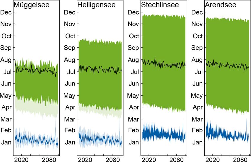
1534                                                T. Shatwell et al.: Future projections of temperature and mixing regime

observed to increase, decrease, or not change with increasing      tion to form) and oligomictic (in lakes too deep for strati-
air temperature (Dokulil et al., 2006; Ficker et al., 2017; Kir-   fication to be destroyed). The fact that climate warming is
illin et al., 2013, 2017; Richardson et al., 2017; Winslow et      likely to shift the mixing regime of some lakes to the right
al., 2017). Stratification strength and duration generally in-     along the polymictic–dimictic–monomictic–oligomictic con-
crease due to warming (Butcher et al., 2015; Kirillin, 2010),      tinuum (Kirillin, 2010; Livingstone, 2008; Shimoda et al.,
but patterns of change may have little regional coherence and      2011) makes understanding the role of the mixing regime
cannot be reliably inferred from surface water trends (Read        all the more important. Still, seasonal warming patterns and
et al., 2014). We know even less about how warming influ-          their role in mediation of the long-term changes remain com-
ences the mixed-layer depth, which is important for instance       paratively unexplored (Winslow et al., 2017).
for light availability for primary production.                         Lake morphology has been identified as a key factor af-
    To better understand the sources of this variability, re-      fecting the seasonal mixing regime (Kraemer et al., 2015;
search has focused on identifying which characteristics mod-       Magee and Wu, 2017) but it cannot explain all the observed
ulate how lakes and particularly lake stratification respond       variance in lake stratification or temperature (Kraemer et al.,
to warming. Recently, a series of modelling studies reported       2015; O’Reilly et al., 2015). Besides morphology, the mix-
the variable regional responses of lakes to projected climate      ing regime depends on climate and water transparency (Kir-
change in the near future (e.g. Boike et al., 2015; Butcher et     illin and Shatwell, 2016) and therefore integrates many of
al., 2015; Dibike et al., 2011; Ladwig et al., 2018; Magee and     the factors that determine how lakes react to climate change.
Wu, 2017; Prats et al., 2018; Woolway et al., 2017). Such          Transparency influences the vertical temperature distribution
regional studies typically focus on the role of lake-specific      by determining how far solar radiation can penetrate into the
factors, such as lake size, morphometry, and water quality         water column. Low transparency generally leads to stronger
in long-term lake trends due to local warming. A consistent        vertical temperature gradients and stratification, a shallower
research extension in this direction could embrace upscal-         mixed-layer depth, and lower deep water and whole-lake
ing to worldwide lake trends in combination with evaluat-          temperatures (Hocking and Straskraba, 1999; Persson and
ing different global change scenarios and (or) different lake      Jones, 2008; Thiery et al., 2014a; Yan, 1983). Decreasing
models. Complementary to this “extensive” approach, lake           transparency (dimming) has been shown to buffer or even
modelling is an efficient tool for generalizing regional stud-     potentially reverse climate-induced trends in mean lake tem-
ies via “intensive” understanding of the energy transport be-      perature (Rose et al., 2016). However, the opposite is true for
tween different temporal scales, which finally produces the        stratification, where warming and dimming effects amplify
integrated effect of slow atmospheric warming on lake dy-          to increase thermal gradients (Kirillin, 2010). The pattern
namics. In this regard, the seasonal variations deserve special    becomes even more complicated with seasonal variations of
attention because they represent the most energetic part of the    the effect of transparency on stratification as well as trans-
entire spectrum both in lakes and in the atmospheric bound-        parency itself (Rinke et al., 2010; Shatwell et al., 2016). A
ary layer. High amplitudes of the seasonal variations involve      major factor determining water transparency is the trophic
the formation of density stratification and ice cover. These       level, which can also experience long-term variations due to
processes are, in turn, governed by different sets of physi-       changing nutrient supply. Thus, the sensitivity of warming to
cal forces at different stages of the seasonal cycle, ensuring     transparency warrants more investigation.
a highly non-linear lake response to atmospheric forcing on            The present study was designed to analyse the effects
longer timescales. In freshwater lakes, the non-linear effects     of seasonality on the response of northern temperate lakes
of seasonality get stronger as the seasonal temperature am-        to projected future warming. We project future changes in
plitudes increase relative to the maximum density value of         thermal characteristics and mixing regime of four temperate
freshwater (∼ 4 ◦ C) and to the freezing point of 0 ◦ C. Hence,    lakes with a thermodynamic model forced by an ensemble of
geographically, seasonality is the strongest in lakes at mid-      climate projections based on a moderate warming scenario,
latitudes, being damped towards tropical and polar regions.        the Representative Concentration Pathway 4.5 (RCP4.5). To
    Seasonal stratification and ice cover prevent certain wa-      differentiate the potential effect of mixing regime on lake re-
ter layers from interacting directly with the atmosphere for       sponse, we simulate two shallow and two deep lakes, where
certain periods of the year, so it follows that the mixing         each pair is similar in terms of morphology but different in
regime should mediate the effect of increasing air temper-         terms of transparency and/or mixing regime. The four lakes
ature on lakes. Major seasonal stratification patterns in fresh-   are located within a distance of ≤ 150 km from each other;
water lakes include dimictic (with lake stratification de-         hence differences in their response to climate change are con-
stroyed twice a year, when lake temperatures cross the max-        ditioned predominantly by lake properties. The aim of our
imum density value) and monomictic (with stratification de-        study is to better understand the internal physical mecha-
stroyed once a year, when surface temperatures decrease to         nisms determining the response of lakes to a future warmer
the maximum density value, but do not reach the freezing           climate by interaction of vertical mixing, ice formation, and
point, so that no stable winter stratification forms), as well     water transparency.
as polymictic (in lakes too shallow for a stable stratifica-

Hydrol. Earth Syst. Sci., 23, 1533–1551, 2019                                   www.hydrol-earth-syst-sci.net/23/1533/2019/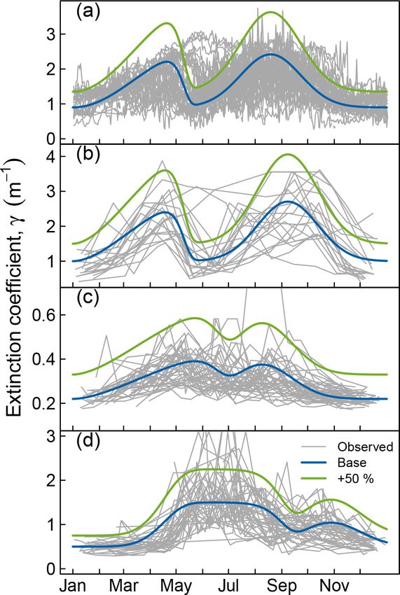
T. Shatwell et al.: Future projections of temperature and mixing regime                                                         1535

Table 1. Characteristics of the four study lakes.

                                                        Müggelsee     Heiligensee    Stechlinsee    Arendsee
                     Mean/max depth (m)                 4.9/8.0       5.9/9.5        23/69          29/51
                     Area (km2 )                        7.3           0.3            4.3            5.1
                     Typical fetch (m)                  4000          1000           2000           4000
                     Secchi depth (m)                   2.0 ± 0.3     1.8 ± 0.4      8.6 ± 0.7      3.0 ± 1.4
                     Mean extinction (m−1 )             1.48 ± 0.31   1.68 ± 0.48    0.29 ± 0.03    0.96 ± 0.55
                     Mean stratification duration (d)   16 ± 7.4      169 ± 17       250 ± 16       232 ± 14
                     Mixing regime                      Polymictic    Dimictic       Dimictic       Di/monomictic
                     Trophic state                      Eutrophic     Hypertrophic   Oligotrophic   Eutrophic

                                                                       able for Müggelsee since 2004. The thermodynamic model
                                                                       was calibrated with long-term temperature measurements
                                                                       from 1979 to 2014 (Müggelsee), 1979 to 2001 (Heiligensee),
                                                                       1991 to 2014 (Stechlinsee), and 1979 to 2010 (Arendsee).
                                                                       Stratification duration measurements in Müggelsee were
                                                                       only based on the high-frequency temperature measurements
                                                                       from 2004 to 2014. Secchi depths (hsecchi ) were measured
                                                                       with a standard 20 cm disk at weekly to monthly inter-
                                                                       vals since at least 1979 in all lakes. Light extinction (γ ) in
                                                                       Müggelsee, Heiligensee, and Stechlinsee was calculated us-
                                                                       ing the Lambert–Beer law from simultaneous light measure-
                                                                       ments at different depths (generally 0.5 m apart) recorded
                                                                       with spherical sensors (Licor, Nebraska). Using regression,
                                                                       we related light extinction to parallel measurements of Sec-
                                                                       chi depth using the relationship γ = c/hsecchi (Poole and
                                                                       Atkins, 1929). We determined the constant c to be 2.05±0.04
                                                                       (mean ± SE, n = 300) for Müggelsee, 2.13 ± 0.10 (n = 52)
Figure 1. Locations of the study lakes in Germany.                     for Heiligensee (Shatwell et al., 2016), and 2.33 ± 0.08 (n =
                                                                       57) for Stechlinsee. In the absence of direct measurements in
                                                                       Arendsee, light extinction was estimated from Secchi depth
2     Methods                                                          measurements as γ = 2.17/hsecchi , where the constant c =
                                                                       2.17 was simply the mean of the estimates from the other
2.1    Study sites                                                     three lakes.

We consider four lakes located in north-eastern Germany in a           2.3   Modelling
temperate continental climate (Fig. 1). Stechlinsee (53.15◦ N,
13.03◦ E) and Arendsee (52.89◦ N, 11.48◦ E) are deep dimic-            Modelling was performed with the lake temperature and mix-
tic groundwater-fed lakes of similar area and depth. Stechlin-         ing model FLake (Kirillin et al., 2011; Mironov, 2008) –
see is oligo-mesotrophic and one of the clearest lakes in the          a bulk model of the lake thermal regime specifically de-
region, whereas Arendsee is eutrophic and turbid (Table 1).            signed to parameterize inland waters in climate models and
Müggelsee (52.44◦ N, 13.65◦ E) is a eutrophic, polymictic              numerical weather prediction systems. FLake is based on a
lake and Heiligensee (52.61◦ N, 13.22◦ E) is a hypertrophic,           two-layer parametric representation of the vertical tempera-
dimictic lake. Both are shallow lakes and located in Berlin.           ture structure. The upper layer is treated as well-mixed and
                                                                       vertically homogeneous. The structure of the lower stably
2.2    Lake data                                                       stratified layer, the lake thermocline, is parameterized us-
                                                                       ing a self-similar representation of the temperature profile.
Long-term water temperature measurements were avail-                   The same self-similarity concept is used to describe the tem-
able at weekly intervals and 0.5 m depth increments for                perature structure of the thermally active upper layer of the
Müggelsee, in bi-weekly to monthly intervals at 1 m depth in-          bottom sediments (Golosov and Kirillin, 2010) and the ice
crements for Heiligensee, and in weekly to monthly intervals           cover (Mironov et al., 2012). The depth of the mixed layer
at varying depth increments in both Stechlinsee and Arend-             is computed from the prognostic entrainment equation in
see. In addition, hourly water temperature profiles were avail-        convective conditions, and from the diagnostic equilibrium

www.hydrol-earth-syst-sci.net/23/1533/2019/                                          Hydrol. Earth Syst. Sci., 23, 1533–1551, 2019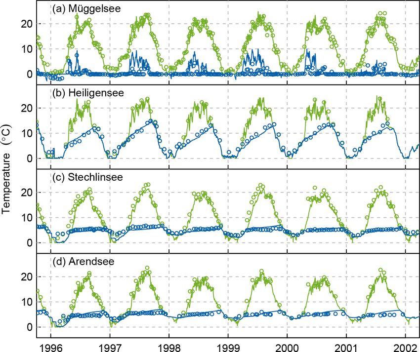
1536                                               T. Shatwell et al.: Future projections of temperature and mixing regime

boundary-layer depth formulation in conditions of wind mix-      increased from 0.04 to 0.22 for the shallow Müggelsee, in
ing against the stabilizing surface buoyancy flux. The inte-     order to mimic the additional vertical mixing produced by
grated approach implemented in FLake allowed high com-           the flow of the River Spree through the lake, which is not
putational efficiency to be combined with a realistic repre-     explicitly accounted for by one-dimensional modelling. The
sentation of the major physics behind turbulent and diffu-       second parameter is the rate of change of the wind-mixed
sive heat exchange in the stratified water column and simi-      layer depth, which is assumed in the model to relax expo-
lar skill compared to other lake models (e.g. Stepanenko et      nentially to the equilibrium depth determined following Zil-
al., 2013, 2014; Thiery et al., 2014b). As a result, FLake is    itinkevich and Mironov (1996). The parameter is suggested
widely used for representing lakes in land schemes of re-        to have the order of magnitude 10−2 (Mironov 2008) and
gional and global climate models, being implemented, for         was set to 0.025 for all lakes based on observed mixed-layer
example, in the surface schemes of the Weather Research          dynamics.
and Forecasting model (WRF, Mallard et al., 2014), Con-
sortium for Small-scale Modelling (COSMO; Mironov et
                                                                 2.4   Climate warming scenarios
al., 2010), HTESSEL (European Centre for Medium-Range
Weather Forecasts, ECMWF; Dutra et al., 2010), SURFEX
(Meteo France; Salgado and Le Moigne, 2010), and JULES           FLake was forced with an ensemble of continuous 21st
(UK Met Office; Rooney and Jones, 2010). Thanks to its ro-       century climate projections from the Coordinated Re-
bustness and computational efficiency, FLake has become the      gional climate Downscaling Experiment for Europe (EURO-
standard choice in climate studies involving the feedbacks       CORDEX; Kotlarski et al., 2014). The climate projections
between inland waters and the atmosphere and is used oper-       were based on an intermediate greenhouse gas concentration
ationally in the NWP models of the German Weather Service        trajectory (RCP4.5), representing a moderate climate warm-
(DWD), the ECMWF, the UK Met Office, the Swedish Me-             ing scenario with an end-of-century, top-of-the-atmosphere
teorological and Hydrological Institute (SMHI), the Finnish      radiative forcing of 4.5 W m−2 compared to the pre-industrial
Meteorological Institute (FMI), and others.                      period (IPCC, 2014). The ensemble was assembled from
   FLake is a process-based model with a high level of pa-       different downscaled global climate models (MPI-ESM-
rameterization, which includes several empirical constants       LR, EC-EARTH, CanESM2, CNRM-CM5, CSIRO-Mk3-6-
estimated from independent observational and numerical           0, GFDL-ESM2M, MIROC5, NorESM1-M) each provid-
data. The model parameterizations have proven reliable in        ing lateral boundary conditions to the RCA4 regional cli-
application to lakes of different morphometry and climatic       mate model. In addition, the MPI-ESM-LR global climate
conditions (Docquier et al., 2016; Kirillin, 2010; Kirillin et   model (GCM) was downscaled by the CCLM4-8-17 and
al., 2013, 2017; Martynov et al., 2010; Shatwell et al., 2016;   REMO2009 regional climate models, and the EC-EARTH
Thiery et al., 2014a, 2015, 2016), so that FLake does not nor-   GCM was downscaled by HIRHAM5 and RACMO22E,
mally require re-tuning for a specific lake. Minor model ad-     yielding an ensemble of 12 climate projections (2006–2100)
justments were performed based on observations. The adjust-      for each lake. The dispersion of mean monthly and annual
ments refer to two model parameters, each of them encom-         air temperature in the ensemble is quite comparable to that
passing multiple effects of lake-specific mechanisms on the      of both the ERA-Interim reanalysis dataset and the observed
thermal stratification.                                          data from a nearby weather station (Fig. 2). The ensemble
   The first parameter is the rate of change of the self-        tended to slightly underestimate the frequency of extremely
similar temperature profile shape under the surface mixed        warm months in the upper 10th percentile (Fig. 2a) but not
layer ϑ(ζ ). It is assumed Rto vary with time, so that the in-   the frequency of warm years (Fig. 2b). All simulations were
                             1
tegral shape factor Cϑ ≡ 0 ϑ(ζ )dζ fluctuates between the        performed at a horizontal resolution of atmospheric forcing
                           max
two asymptotic bounds Cϑ and Cϑmin with a characteristic         data of 0.44◦ . For the analysis we selected the model pixel
timescale t∗ as                                                  containing the lake under consideration.
dCϑ  C max − Cϑmin
    ∝ ϑ            .                                       (1)
 dt        t∗                                                    2.5   Temporal downscaling of meteorology
The parameterization incorporates mixing in the lower strati-
fied layer (hypolimnion) by intermittent shear turbulence and    The FLake forcing variables included solar radiation (IR ),
breaking internal waves. The timescale t∗ is parameterized as    near-surface air temperature (Ta ), 10 m wind speed (U10 ),
a function of the thickness of the hypolimnion, the strength     specific humidity (ea ), and cloud fraction (N ). These vari-
of stratification across it, and the rate of mixing at the top   ables were available at daily resolution in the climate pro-
of the thermocline (see Mironov, 2008, for details). Obser-      jections and were downscaled for model simulations to 6-
vational data on temporal variations of Cϑ in several lakes      hourly resolution with the same daily mean to account for
demonstrated that t∗ tends to vary among them depending on       diurnal forcing. Solar radiation and wind speed were down-
lake depth (Kirillin, unpublished data). This parameter was      scaled assuming a sine course during the day, with a constant

Hydrol. Earth Syst. Sci., 23, 1533–1551, 2019                                 www.hydrol-earth-syst-sci.net/23/1533/2019/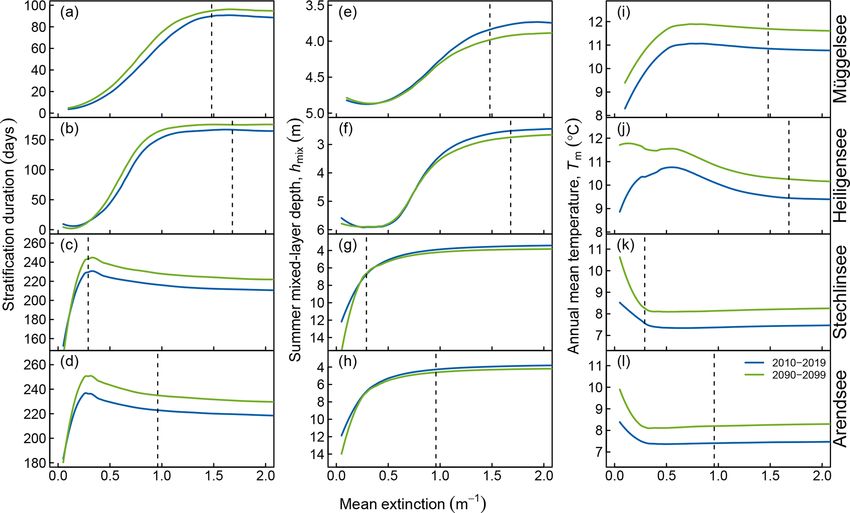
T. Shatwell et al.: Future projections of temperature and mixing regime                                                         1537

                                                                      a prescribed daily mean p from the climate projections is
                                                                      given by calculating pmax with Eq. (3) and substituting it
                                                                      into Eq. (2). For wind speed, the daily course is defined
                                                                      from the daily mean given the daily amplitude pmax − pmin ,
                                                                      which was empirically estimated from the Menz weather data
                                                                      and varied seasonally. Random Gaussian noise was added
                                                                      to wind speeds with the same variability (variance propor-
                                                                      tional to mean) as observed in the Menz station. This method
                                                                      accurately reproduced the complexity of the observed wind
                                                                      speed dynamics: It produced realistic behaviour of day-to-
                                                                      day wind speed (Fig. 3a), as well as the diurnal variation of
                                                                      mean wind speed and associated variance (Fig. 3b, c), and
                                                                      also the seasonal change of this diurnal variation (Fig. 3b, c),
                                                                      while still preserving the given daily mean wind speeds. Sub-
                                                                      daily air temperatures were interpolated between a daytime
                                                                      maximum assumed at 14:00 LT and night-time minimum as-
                                                                      sumed at 02:00 LT using a cubic spline, where the daily tem-
                                                                      perature amplitude 1Ta (K) was estimated from the daily
                                                                      mean temperature Ta (◦ C) using the empirical relationship
                                                                      1Ta = 0.345Ta + 5.5 based on the Menz data. Sub-daily hu-
Figure 2. Cumulative distribution function of centred                 midity and cloud fraction were linearly interpolated between
monthly (a) and annual mean air temperature (b), based on             the daily mean values.
data from 1991 to 2010. The grey lines show the 12 historical
scenarios in the ensemble, the green line shows ERA-Interim           2.6   Extinction scenarios
reanalysis data, and the blue line shows the observed data from the
Menz weather station. All data are for the closest pixel or weather   We performed lake model simulations with different scenar-
station to Stechlinsee.                                               ios of seasonal extinction, which in these lakes is primar-
                                                                      ily determined by phytoplankton chlorophyll (Shatwell et al.,
minimum value during the night, according to the model:               2016). Here the thermodynamic model was modified to ac-
                                                                      count for seasonally variable extinction, following a typical
                      π (t − lag − trise ) m

                                                                      bimodal pattern according to the Plankton Ecology Group
p = pmin + pmax sin                          ,
                          tset − trise                                (PEG) model (Sommer et al., 1986, 2012), as described in
 p ≥ pmin ≥ 0,                                          (2)           detail in Shatwell et al. (2016). A base seasonal extinction
                                                                      pattern was derived from long-term observations of extinc-
where p is the solar radiation or wind speed as a function            tion and/or Secchi depth in each study lake, preserving im-
of time of day (t, in hours); pmin and pmax are the night-            portant seasonal characteristics including long-term annual
time minimum and daytime maximum values, respectively;                mean extinction (see Table 1), minimum extinction, and tim-
trise and tset are the times of sunrise and sunset, respectively;     ing and magnitude of the spring and summer blooms (Fig. 4).
lag is the time lag of the maximum value behind solar noon            The spring and summer blooms were described by Weibull
(halfway between trise and tset ); and m is a shape constant.         and Gauss curves, respectively.
The constant m was empirically determined to be 1.3 based                Using these base extinction patterns as the control sce-
on high-resolution weather data (1 November 1991 to 24 Au-            nario, we simulated the hydrodynamics of the four lakes
gust 2004) from the Menz weather station 5 km from Lake               for the period 2006–2100 forced by the climate projection
Stechlin (Fig. 1). Sunrise and sunset times were determined           ensemble. To test the sensitivity of lake warming response
at the coordinates of each study lake on each day of the year         to water clarity, we then repeated these simulations with a
with a NOAA algorithm using the R package maptools (Bi-               modified mean extinction coefficient. The mean extinction
vand and Lewin-Koh, 2016). The daily mean is given by                 coefficient was varied by scaling the whole seasonal extinc-
                                                                      tion pattern, affecting mean, minimum, and peak extinction
                          (tset − trise )
p = pmin + (pmax − pmin )                 0                           equally. A principal component analysis on long-term extinc-
                             24                                    tion coefficient measurements in Müggelsee and Heiligensee
    m + 1 √ m             −1
                                                                      showed that this method best represented the natural varia-
              π0     +1          .                             (3)
      2            2                                                  tion in the seasonality of extinction (Shatwell et al., 2016).
For solar radiation, lag = 0 and pmin = 0. For wind speed,
lag = 1 h based on empirical observations and pmin is non-
zero. Accordingly, the daily course of solar radiation p for

www.hydrol-earth-syst-sci.net/23/1533/2019/                                        Hydrol. Earth Syst. Sci., 23, 1533–1551, 2019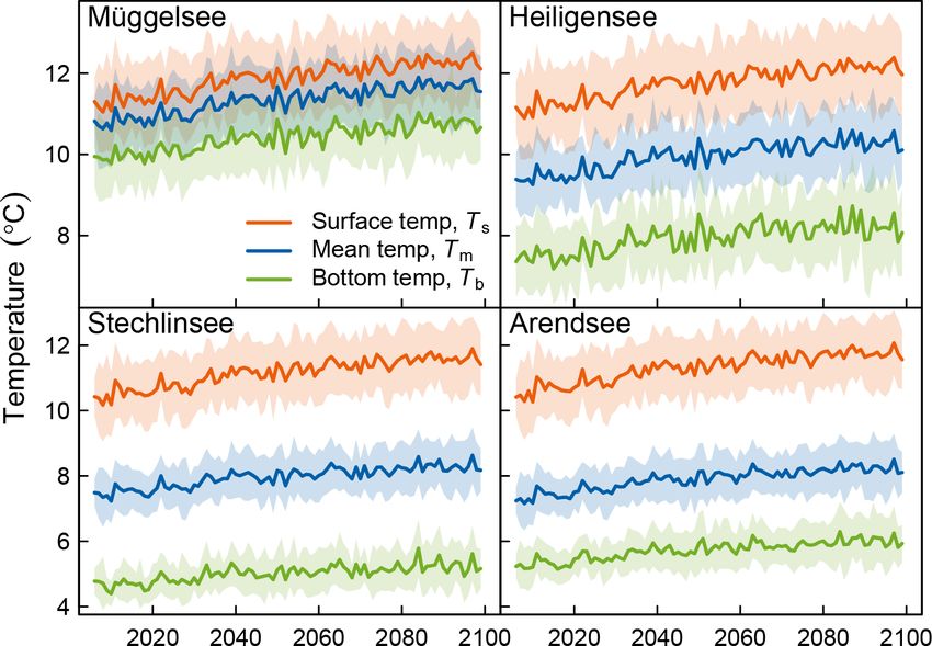
1538                                                  T. Shatwell et al.: Future projections of temperature and mixing regime

                                                                     Figure 4. Seasonal course of extinction (γ ) in Müggelsee (a), Heili-
                                                                     gensee (b), Stechlinsee (c), and Arendsee (d). Grey lines show su-
                                                                     perimposed observed extinction during individual years, thick blue
                                                                     lines show the idealized seasonal course of extinction used in model
                                                                     simulations with FLake (base scenario). Green lines show base
                                                                     extinction increased by 50 %. Panels (a) and (b) modified from
Figure 3. Comparison of disaggregated and observed sub-daily         Shatwell et al. (2016).
wind speeds at the Menz weather station (5 km from Stechlin-
see): sample of observed hourly wind data from 1998 and the dis-
aggregated wind speeds generated from the corresponding daily
means (a); hourly mean and standard deviation of observed (cir-      teorology, as the future projections are obtained by forcing
cles, shaded area) and disaggregated wind speeds (solid and dashed   FLake with a gridded simulation product rather than in situ
lines) in February (b) and July (c).                                 information, and (ii) the EURO-CORDEX reanalysis down-
                                                                     scaling simulations, as calibrated model parameters would in
                                                                     that case differ between model projections. For consistency
2.7    Model set-up and calibration                                  the ERA-Interim-driven simulations were downscaled from
                                                                     daily means to sub-daily values using the same procedure as
FLake was configured for each lake by setting mean lake              for the climate projections described above. Using a model
depth and fetch, the temperature at the bottom of the ther-          calibrated on a different dataset (ERA-Interim) than the cli-
mally active sediment layer (set to the historical long-term         mate projections can introduce bias into the results. Thus we
mean water temperature at the lake bottom), and the extinc-          reran the model calibrated on ERA-Interim data with forcing
tion coefficient as described above. The model was man-              from the historical hindcasts of each of the 12 GCM–RCM
ually calibrated for each lake by adjusting t∗ with a con-           combinations in the ensemble. The mean bias of each vari-
stant. Additionally, in the case of shallow Müggelsee, the           able forced by the ensemble hindcast barely differed from
rate of change of the mixed-layer depth due to wind forc-            the bias obtained using ERA-Interim forcing. In fact, the en-
ing was changed to account for the additional vertical mix-          semble showed on average a smaller absolute bias in bot-
ing produced by the riverine throughflow (see Sect. 2.3 for          tom temperature, mixed-layer depth, stratification duration
details). Hindcast simulations were forced with meteorology          and stratification onset timing and a slightly greater bias only
from ERA-Interim gridded reanalyses produced by the Eu-              in surface temperature and stratification breakdown timing.
ropean Centre for Medium-Range Weather Forecasts (Dee et             Therefore, our simulations are largely unaffected by bias.
al., 2011). Using this meteorological forcing as a basis for            Precipitation, including snow cover on ice, was not in-
the model calibration was preferred over using (i) in situ me-       cluded in modelling. There are several indications suggest-

Hydrol. Earth Syst. Sci., 23, 1533–1551, 2019                                       www.hydrol-earth-syst-sci.net/23/1533/2019/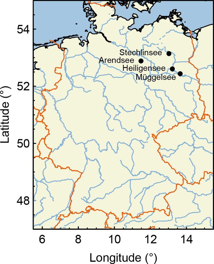
T. Shatwell et al.: Future projections of temperature and mixing regime                                                             1539

Figure 5. Comparison of modelled (lines) and observed temperatures (points) in Müggelsee (a), Heiligensee (b), Stechlinsee (c), and Arend-
see (d). Green lines and symbols show surface temperatures, blue lines and symbols show bottom temperatures (b–d) or surface–bottom
temperature differences (a).

ing that including the snow as model input would not im-               sured weekly, and from 2004 to 2014 hourly), from 1979 to
prove the predictive value of the model outcomes. Firstly,             2001 in Heiligensee (monthly), from 1991 to 2012 in Stech-
the current version of FLake treats the thermal regime under           linsee (weekly to monthly), and from 1979 to 2010 in Arend-
ice in a simplified way, without taking into account the short-        see (weekly to monthly). As different measures of goodness
wave radiation penetrating into the water column under the             of fit, we examined model bias (Eq. 4), centred root mean
ice cover. Therefore including the insulating effect of snow           square error (RMSEc , Eq. 5), normalized root mean square
on the radiation flux would not substantially change the mix-          error (RMSEn , Eq. 6), and normalized standard deviation
ing physics of the ice-covered period. Secondly, in temperate          (σnorm , Eq. 7), where mi and oi are the modelled and ob-
regions, the relatively short ice-covered periods on lakes are         served values, respectively, and (m) and (o) are their means:
weakly affected by the snow cover compared to, for exam-
ple, boreal and arctic lakes. This fact was also supported by          bias = m − o,                                                  (4)
the study of the FLake performance for the ice modelling on
                                                                                 v
                                                                                 u n
                                                                                 u1 X
Lake Müggelsee (Bernhardt et al., 2012). Moreover, we did              RMSEc = t          ((mi − m) − (oi − o))2 ,                    (5)
not account for changes in inflow because our focus was on                          n i=1
lake–atmosphere interactions. Instead we assessed the sen-                       v
                                                                                 u n
                                                                                                      v
                                                                                                      u n
sitivity of the lakes to a change in transparency, which can                     u1 X               2 t1
                                                                                                     u X
                                                                       RMSEn =   t        (oi − mi )             o2 ,                 (6)
be expected if warming alters runoff as well as nutrient and                        n i=1                n i=1 i
carbon export.                                                                 v
   Model performance was assessed by comparing the mod-                        u n
                                                                               uX              X  n
elled and observed surface temperature (Ts ), bottom tempera-          σnorm = t (mi − m)2           (oi − o)2 .                      (7)
ture (Tb ), and, for the seasonally stratified lakes (Heiligensee,                  i=1              i=1
Stechlinsee, and Arendsee), the mean summer mixed-layer
depth (hmix ) and timing and duration of seasonal stratifica-          2.8   Data handling and statistics
tion. Here we assessed model performance using temperature
                                                                       Ts was calculated from field data as the mean temperature in
profiles in the period from 1979 to 2014 in Müggelsee (mea-
                                                                       the 0–1 m layer. Tb was calculated as the mean temperature at

www.hydrol-earth-syst-sci.net/23/1533/2019/                                          Hydrol. Earth Syst. Sci., 23, 1533–1551, 2019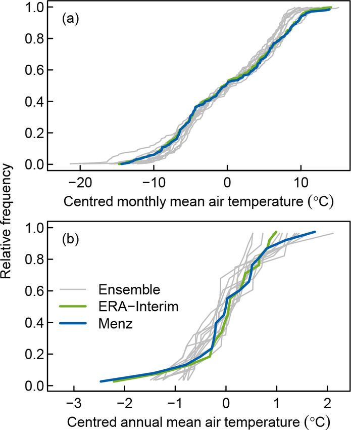
1540                                                 T. Shatwell et al.: Future projections of temperature and mixing regime

                                                                    close to 1, except in bottom temperatures of the two deep
                                                                    lakes Stechlinsee and Arendsee, which are quite invariant
                                                                    with a standard deviation of 0.86 and 0.99 ◦ C respectively.
                                                                    However, the model had a systematic tendency to underesti-
                                                                    mate Ts in all lakes by 0.7–1.8 ◦ C. The model also adequately
                                                                    reproduced the stratification characteristics of the three sea-
                                                                    sonally stratified lakes with a centred error of 1–2 m for hmix
                                                                    and about 2–3 weeks for stratification duration, noting that
                                                                    the sampling interval (and thus measurement error) for strat-
                                                                    ification duration was generally 4 weeks. The model system-
                                                                    atically underestimated the stratification duration by about
                                                                    1 month, probably because the surface temperatures were
Figure 6. Projected changes in over-lake near-surface air temper-   also underestimated.
ature under RCP4.5. Lines show decadal means over all climate
projections and all four locations.                                 3.2   Meteorology trends

                                                                    Air temperatures in the RCP4.5 forcing ensemble in-
the mean depth of each lake. Stratification was inferred when
                                                                    creased on average by 0.16 ◦ C per decade over all
the absolute difference between Ts and Tb exceeded 0.5 ◦ C.
                                                                    lakes. These increases were strongest in winter and
The lake was assumed to be mixed when it was not strati-
                                                                    spring (0.23–0.30 ◦ C decade−1 ) and weakest in summer
fied. The duration of seasonal stratification was defined as the
                                                                    (0.04 ◦ C decade−1 , Fig. 6). Mean annual radiation decreased
length of the longest uninterrupted stratification period each
                                                                    in the ensemble by 0.29 W m−2 decade−1 . The overall de-
season. Similarly, the duration of overturn was defined as the
                                                                    crease was unevenly distributed seasonally, with a strong
length of the longest uninterrupted period of mixing in each
                                                                    decrease projected for summer (1.65–1.70 W m−2 decade−1 )
season following the main stratification events. Winter was
                                                                    but an increase projected for winter (1.1 W m−2 decade−1 ).
defined as January to March, spring as April to June, sum-
                                                                    Annual mean water vapour pressure was projected to in-
mer as July to September, and autumn as October to Decem-
                                                                    crease by 0.1 Pa decade−1 with stronger increases in win-
ber. Trends were assessed using linear regression over time.
                                                                    ter and spring than in summer and autumn. The projected
Differences between transparency treatments were assessed
                                                                    changes in wind speed were negligible.
by comparing decadal means of a particular variable for each
climate projection in the ensemble, yielding 12 means per
decade over 9 decades from 2010 to 2100. Comparisons were           3.3   Lake response to warming
made using ANCOVA with decade as the covariate. Normal-
ity of residuals was assessed with quantile–quantile plots, ho-     In model runs with the historical, baseline extinction, these
mogeneity of variance with plots of residuals versus fitted         projected climate trends resulted in an increase in annual sur-
values, and outliers with plots of Cook’s distances. Increas-       face water temperatures (higher rates of increase in deeper
ing variance with the mean was resolved by log transforma-          lakes) in all lakes for the simulation period 2006–2100
tion. Ice-cover duration was extended by 1 day to avoid zero        (Fig. 7, Table 3). Bottom temperatures increased in all lakes,
values before log transformation. Outliers with a Cook’s dis-       with faster warming rates projected in the two shallower
tance > 1 were excluded from statistical analyses. Small devi-      lakes Müggelsee and Heiligensee. Accordingly, mean lake
ations from normality were tolerated. All statistical analyses      temperatures increased in all lakes at 0.10–0.11 ◦ C decade−1 .
were performed with R version 3.3.0 (R Core Team, 2016).               Ts increased most rapidly during the winter in the two shal-
                                                                    lower lakes and during spring in the two deeper lakes. On
                                                                    the other hand, mean summer Ts increased only marginally
3     Results                                                       in Stechlinsee (0.02 ◦ C decade−1 ) and not at all in the other
                                                                    lakes (Fig. 8). Tb increased most rapidly in winter. Moreover,
3.1    Model validation                                             the higher Tb in April and May, when stratification typically
                                                                    began, persisted until the end of stratification (September in
The thermodynamic model forced by the ERA-Interim re-               Heiligensee and November–December in deeper Stechlin-
analysis data performed well at reproducing the observed            see and Arendsee; Fig. 8). Accordingly, deep water warmed
thermodynamic characteristics of the study lakes (Fig. 5).          faster than surface water during summer (and autumn in the
The model predicted water temperature with good precision           deep lakes), which led to a lower vertical temperature gradi-
as evident in RMSEc values generally less than 1.5 ◦ C for          ent in summer, and consequently weaker stratification. Fur-
surface and bottom temperatures (Table 2). The model also           thermore, annual maximum surface temperature increased
reproduced observed temperature variability well with σn            and occurred earlier in summer (Fig. 9, Table 3).

Hydrol. Earth Syst. Sci., 23, 1533–1551, 2019                                    www.hydrol-earth-syst-sci.net/23/1533/2019/
T. Shatwell et al.: Future projections of temperature and mixing regime 1541
Table 2. Goodness-of-fit statistics of the four study lakes. Stratification statistics not shown for polymictic Müggelsee.
Lake Bias RMSEc RMSEn σn n
Ts Müggelsee −0.67 1.02 0.07 1.13 1335
Heiligensee −1.07 1.04 0.09 1.18 383
Stechlinsee −1.83 1.43 0.13 1.23 482
Arendsee −1.06 1.46 0.11 1.13 445
Tb Müggelsee −1.72 1.94 0.15 1.13 1303
Heiligensee −1.22 1.46 0.17 0.95 383
Stechlinsee −0.29 0.62 0.13 1.93 482
Arendsee 0.22 0.95 0.19 2.45 444
hmix Heiligensee −1.56 0.95 0.43 0.85 113
Stechlinsee 1.20 1.55 0.28 0.66 191
Arendsee −2.1 2.0 0.42 0.36 134
Stratification duration Heiligensee −35.3 17.2 0.16 0.60 21
Stechlinsee −39.4 15.5 0.17 0.73 33
Arendsee −21.2 12.0 0.11 0.74 19
Stratification begin Heiligensee 8.6 10.8 0.14 0.52 21
Stechlinsee 16.9 10.2 0.20 0.63 22
Arendsee 5.8 8.7 0.10 0.93 24
Stratification end Heiligensee −1.9 16.3 0.06 0.69 20
Stechlinsee −18.5 9.6 0.06 0.58 21
Arendsee −15.3 11.5 0.06 0.30 21
Ice duration Müggelsee −29.9 22.8 0.64 0.14 23
Stechlinsee −21.1 24.7 0.81 0.07 13
Figure 7. Projected evolution of surface, mean, and bottom temperatures in the four study lakes. Shading indicates 1 standard deviation
either side of the mean.
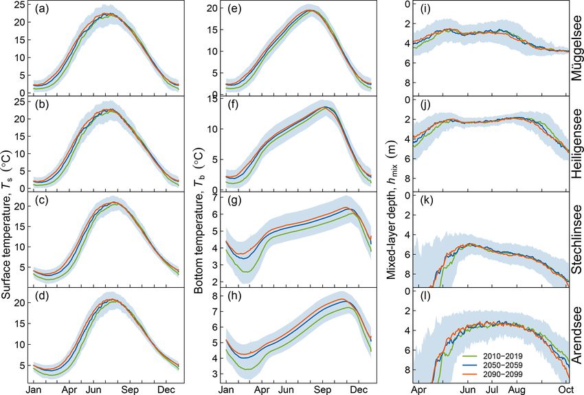
www.hydrol-earth-syst-sci.net/23/1533/2019/ Hydrol. Earth Syst. Sci., 23, 1533–1551, 20191542 T. Shatwell et al.: Future projections of temperature and mixing regime Figure 8. Modelled seasonal cycle of surface (a–d) and bottom temperature (e–h) and mixed-layer depth (i–l) in Müggelsee (a, e, i), Heiligensee (b, f, j), Stechlinsee (c, g, k), and Arendsee (d, h, l). Lines indicate decadal means and shading denotes 1 standard deviation each side of the mean. Figure 9. Projected trends in stratification in the four study lakes. Green shading shows summer stratification, blue shows winter stratification. Lighter shading indicates intermittent stratification. The black line shows the timing of maximum surface temperature. The model was forced with the baseline (historical) transparency. Hydrol. Earth Syst. Sci., 23, 1533–1551, 2019 www.hydrol-earth-syst-sci.net/23/1533/2019/
T. Shatwell et al.: Future projections of temperature and mixing regime                                                                 1543

Table 3. Projected trends (2006–2100) in lake temperature and stratification characteristics, with 95 % confidence intervals in parentheses.
Italics denote trends with 0.01 < p < 0.05; all other trends are significant at p < 0.001; doy: day of the year; ns: not significant.

                       Unit decade−1     Müggelsee                Heiligensee             Stechlinsee             Arendsee
    Surface
    temperature
    Annual             ◦C                0.12 (0.11 to 0.14)      0.13 (0.11 to 0.14)     0.14 (0.12 to 0.15)     0.14 (0.13 to 0.16)
    Winter             ◦C                0.25 (0.23 to 0.27)      0.26 (0.24 to 0.28)     0.21 (0.19 to 0.23)     0.20 (0.18 to 0.23)
    Spring             ◦C                0.22 (0.19 to 0.24)      0.23 (0.20 to 0.25)     0.30 (0.28 to 0.33)     0.31 (0.29 to 0.34)
    Summer             ◦C                ns                       ns                      0.02 (0.00 to 0.05)     ns
    Autumn             ◦C                0.02 (0.00 to 0.05)      0.02 (0.00 to 0.04)     ns                      0.03 (0.01 to 0.04)
    Maximum            ◦C                0.13 (0.09 to 0.17)      0.12 (0.08 to 0.16)     0.14 (0.11 to 0.17)     0.13 (0.10 to 0.16)
    Timing of          doy               −1.0 (−1.4 to −0.6)      −0.8 (−1.2 to −0.4)     −1.1 (−1.5 to −0.7)     −0.9 (−1.3 to −0.6)
    maximum
    Bottom
    temperature
    Annual             ◦C                0.10 (0.09 to 0.12)      0.10 (0.08 to 0.11)     0.07 (0.06 to 0.08)     0.08 (0.07 to 0.10)
    Winter             ◦C                0.20 (0.18 to 0.22)      0.18 (0.16 to 0.20)     0.12 (0.10 to 0.13)     0.11 (0.10 to 0.13)
    Spring             ◦C                0.17 (0.15 to 0.20)      0.12 (0.09 to 0.15)     0.06 (0.05 to 0.08)     0.08 (0.07 to 0.10)
    Summer             ◦C                ns                       0.06 (0.04 to 0.09)     0.05 (0.04 to 0.07)     0.09 (0.08 to 0.10)
    Autumn             ◦C                0.02 (0.002 to 0.04)     0.02 (0.00 to 0.04)     0.04 (0.03 to 0.06)     0.06 (0.04 to 0.07)
    Summer
    stratification
    Duration           d                 0.8 (0.4 to 1.3)         0.9 (0.5 to 1.2)        1.8 (1.4 to 2.1)        1.6 (1.3 to 1.9)
    Start timing       doy               −1.5 (−1.9 to −1.0)      −1.5 (−1.8 to −1.2)     −2.1 (−2.4 to −1.9)     −2.2 (−2.5 to −2.0)
    End timing         doy               ns                       −0.7 (−0.9 to −0.4)     −0.4 (−0.6 to −0.2)     −0.7 (−0.9 to −0.5)
    Summer mixed-      m                 0.02 (0.01 to 0.02)      0.03 (0.02 to 0.04)     ns                      0.04 (0.03 to 0.04)
    layer depth
    Winter
    stratification
    Duration           d                 −0.9 (−1.2 to −0.6)      −1.1 (−1.4 to −0.8)     −1.7 (−2.2 to −1.3)     −2.0 (−2.5 to −1.6)
    Start timing       doy               −0.8 (−1.4 to −0.3)      −1.0 (−1.5 to −0.5)     ns                      −0.7 (−1.2 to −0.1)
    End timing         doy               −1.2 (−1.8 to −0.6)      −1.4 (−1.9 to −0.8)     −1.6 (−2.2 to −1.1)     −2.3 (−3.0 to −1.6)
    Ice cover
    Duration           d                 −0.9 (−1.1 to −0.6)      −1.0 (−1.3 to −0.7)     −0.4 (−0.5 to −0.3)     −0.2 (−0.3 to −0.1)
    First freeze       doy               ns                       ns                      ns                      ns
    Last thaw          doy               −1.4 (−2.1 to −0.6)      −1.4 (−2.1 to −0.7)     −1.8 (−2.8 to −0.9)     ns

   Winter and spring warming caused stratification to begin             Interestingly, most of the changes in winter stratification and
earlier in all lakes in the model simulations (Fig. 9). This was        ice cover were projected to occur in the first half of the 21st
also reflected in a shallower mean hmix during spring in the            century, with little change in the second half.
deep lakes Stechlinsee and Arendsee. The end of stratifica-                The projected increase in stratification duration was in-
tion also advanced slightly due to the slightly smaller ver-            sufficient to cause Müggelsee to stratify continuously from
tical temperature gradients in summer, but not as rapidly as            spring to the end of summer (median duration in the decade
stratification onset, so that overall stratification duration in-       2090–2099: 102 days) and thus shift from a polymictic to
creased. Mean summer hmix increased in three lakes by less              a dimictic regime. On the other hand, the deeper dimictic
than 0.05 m decade−1 , which is practically negligible. Win-            lakes Stechlinsee and Arendsee were projected to be at the
ter stratification and ice cover were more intermittent in the          transition to a monomictic regime by the middle of the 21st
two shallow lakes than in the two deeper lakes. Winter and              century. In the decade 2050–2059, the model projected that
spring warming mainly caused winter stratification and ice              Stechlinsee and Arendsee would have no winter stratifica-
cover to end earlier, reducing the overall duration (Fig. 9).           tion in 33 % and 55 % of winters and be ice-free in 76 % and

www.hydrol-earth-syst-sci.net/23/1533/2019/                                             Hydrol. Earth Syst. Sci., 23, 1533–1551, 2019
1544 T. Shatwell et al.: Future projections of temperature and mixing regime
Figure 10. Interacting effects of extinction and warming on stratification duration (a–d), mean mixed-layer depth in summer (e–h), and
annual mean temperature (i–l) in Müggelsee (a, e, i), Heiligensee (b, f, j), Stechlinsee (c, g, k), and Arendsee (d, h, l). Lines have been loess-
smoothed and show ensemble means for the decades 2010–2019 (blue) and 2090–2099 (green) as a function of extinction. Black vertical
dashed lines show the long-term measured extinction in each lake.
93 % of winters, respectively. By comparison, in the decade to lake type. There were transparency ranges where trans-
2010–2019, Stechlinsee and Arendsee were projected to have parency had a very large effect on thermal structure, and
no winter stratification in 13 % and 24 % of winters and be ranges where it had little effect at all. In general, changes
ice-free in 58 % and 75 % of winters, respectively. The mean in transparency had a strong effect on stratification dura-
winter bottom temperature in the decade 2090–2099 was tion and vertical temperature structure at intermediate ex-
projected to be 3.96 ± 0.93 ◦ C in Stechlinsee (compared to tinction (ca. 0.4–1.1 m−1 ) in the moderately shallow lakes
3.03 ± 0.79 ◦ C in 2010–2019) and 4.48 ± 0.93 ◦ C in Arend- Müggelsee and Heiligensee (Fig. 10a, b) and at very low ex-
see (compared to 3.62 ± 0.73 ◦ C in 2010–2019). tinction (< 0.3 m−1 ) in the deep lakes Stechlinsee and Arend-
Annual mean whole-lake water temperature correlated see (Fig. 10c, d). Outside these ranges, changes in extinc-
with annual mean air temperature. At any given annual mean tion had a much smaller effect: at extinctions above about
air temperature, Müggelsee was warmest, followed by Heili- 1.1 m−1 in the two shallower lakes (or > 0.3 m−1 in Stech-
gensee, Stechlinsee, and Arendsee. Moreover, at a given an- linsee) a further increase in extinction no longer increased
nual mean air temperature, all lakes were colder following stratification duration, but rather decreased it gradually due
winters with ice cover than without ice cover, where the tem- to a very gradual increase in summer bottom temperatures.
perature differences increased with mean lake depth. Accordingly, at extinction values higher than the histori-
cal means in the four study lakes (vertical dashed lines in
3.4 Interaction between warming and transparency Fig. 10; see also Table 1), the trends in stratification dura-
tion due to warming were stable and relatively insensitive
to changes in transparency. Thus, an increase in extinction
To investigate the sensitivity of different lake types to a
combined with warming is unlikely to push Müggelsee from
change in transparency combined with warming, we mod-
a polymictic to a dimictic regime. However, the simulations
elled the projected warming effects (2006–2100) in the given
also suggested that clearer shallow lakes, which are close to
lakes with mean extinction ranging from extremely clear
the transition between polymictic and dimictic regimes, can
(γ = 0.05 m−1 ) to extremely turbid (γ = 3 m−1 ). The ef-
potentially switch mixing regimes because interactions be-
fect of transparency and its interactions with warming were
tween warming and dimming are stronger. Altogether, the
highly non-linear and the responses were very sensitive
Hydrol. Earth Syst. Sci., 23, 1533–1551, 2019 www.hydrol-earth-syst-sci.net/23/1533/2019/T. Shatwell et al.: Future projections of temperature and mixing regime 1545
model suggested that changes in stratification duration due
to changes in transparency can be expected at optically nor-
malized depths γ × hmean < 5 to 8 (Fig. 11). Figure 11 was
derived for the period 2090–2099. Although stratification du-
ration increased over time as indicated in Table 3, the relative
dependence on extinction was similar during the whole pe-
riod covered in the ensemble.
The model predicted that an increase in extinction in the
four study lakes above their historical values would not in-
fluence whole-lake warming rates (Tm ) induced by climate
change (Fig. 10i–l). However, the model did suggest that
there would be an interaction between warming and dimming
at extinctions considerably lower than the historical extinc-
tion values observed in these lakes. In the deep lakes, dim- Figure 11. Stratification duration vs. optically normalized depth
ming was predicted to decrease Tm at extinctions below about (mean extinction (γ , m−1 ) × mean depth (hmean , m), dimension-
0.3 m−1 (Fig. 10c, d). According to simulations, increasing less) in lakes Müggelsee, Heiligensee, Stechlinsee, and Arendsee.
extinction from 0.1 to 0.3 m−1 would approximately cancel The curves are loess-smoothed and are based on ensemble simula-
tions with the baseline extinction in each lake for the 2090–2099
out the expected effect on Tm of 90 years of climate warming.
period.
The shallower lakes behaved differently to the deep lakes at
low extinction. In Müggelsee, Tm increased with increasing
extinction up to about 0.5 m−1 (Fig. 10a). In Heiligensee the
model suggested a strong interaction between warming and other seasons. In fact, our projections suggest that the study
dimming up to an extinction of about 0.5 m−1 , where dim- lakes will warm predominantly in winter and spring, and only
ming would decrease Tm in the warmer climate at the end marginally in summer and autumn. These seasonal patterns
of the 21st century but increase Tm in the cooler climate of largely reflect the seasonality of air temperature trends in the
today (Fig. 10b). warming ensemble. The model may have slightly underesti-
Whereas the model predicted that warming would have a mated the increase in summer peak temperatures and occur-
small (deepening) effect on mixed-layer depth, it predicted rence of extended stratification during heatwaves in polymic-
that an increase in extinction would have a stronger (shoal- tic Müggelsee because the ensemble tended to slightly un-
ing) effect (Fig. 10e–h). Again, a change in extinction would derestimate the frequency of extremely warm months. The
have a much stronger effect on the mixed-layer depth at in- leftward seasonal skew of surface water temperature increase
termediate extinctions in the shallower lakes and at a low towards spring and our estimates that the summer maximum
extinction in the deep lakes. temperature should occur increasingly earlier in the year im-
ply that the number of days per year when the surface tem-
perature exceeds a certain threshold will increase. Accord-
4 Discussion ingly, although summer warming was slow, the length of the
bathing season will likely increase and along with it both the
4.1 Warming trends
recreational value and the recreational pressure on lakes.
Our projections suggest that surface waters in all modelled Stratification and ice cover restrict vertical heat trans-
lakes will warm at about 75 %–90 % of the rate of air temper- port and thus influence heat storage in lakes. Therefore they
ature increase, with surface temperatures in the deeper lakes should modulate how lakes respond to warming. This was ev-
increasing faster than the shallower lakes. This is similar to ident in our simulations because, at the same annual mean air
other modelling studies based on climate projections, which temperature, lakes were colder in years with ice cover (dim-
found warming rates of 70 %–85 % of air temperature trends ictic regime) than in years without ice (monomictic regime).
(Butcher et al., 2015; Schmid et al., 2014). The relatively uni- This can be explained in part by the thermal inertia from the
form results obtained from climate and lake modelling stud- previous season (Crossman et al., 2016), and in part due to
ies are not entirely consistent with empirical evidence, which altered heat accumulation in deep water during mixing pre-
shows that warming rates of surface water relative to air can ceding summer stratification. The latter was demonstrated
be more variable (O’Reilly et al., 2015; Torbick et al., 2016). by the relatively steep trends in bottom temperature during
winter simulated in the four study lakes. These effects were
4.2 Influence of seasonality and stratification also observed empirically in Stechlinsee, which was ther-
mally polluted by a nuclear power plant, preventing ice cover
We found that seasonality of warming played an important and shifting the mixing regime from dimictic to monomic-
role and we concur with Winslow et al. (2017) that sum- tic (Kirillin et al., 2013). Here the waste heat input during
mer lake warming rates are not representative of warming in winter mixing was stored in deep water until the following
www.hydrol-earth-syst-sci.net/23/1533/2019/ Hydrol. Earth Syst. Sci., 23, 1533–1551, 20191546 T. Shatwell et al.: Future projections of temperature and mixing regime
winter and increased the mean lake temperature, whereas the Adrian, 2009). The warming effect on stratification dura-
waste heat input during stratification was confined to the sur- tion and mixed-layer depth was relatively small in compar-
face layer and quickly lost to the atmosphere. The effect of ison with the potential effect of a change in transparency
summer stratification on heat transport and storage explains (Fig. 10a, e). Thus, lakes at the transition between polymic-
why the simulated mean lake temperature increased faster tic and dimictic regimes may shift more due to changes in
in the polymictic lake Müggelsee than in seasonally strati- transparency or water level than due to warming alone.
fied Heiligensee, although these lakes have very similar mean
depths. We conclude that not just morphology, but also mix- 4.4 Mixed-layer depth
ing regime modulates how lakes respond to climate warming.
Moreover, we conclude that seasonal differences in climate An important question that has not been conclusively an-
warming rates combined with the strongly non-linear sen- swered is how climate change will affect the mixed-layer
sitivity of lakes to monthly temperature changes determine depth. Our simulations suggested that climate warming
how lakes react to warming overall. would increase the mixed-layer depth in stratified lakes, but
the projected increase of less than 0.05 m decade−1 should
4.3 Mixing regime shifts be considered negligible. Other lake model simulations have
also predicted that the mixed layer will deepen with warm-
The comparatively rapid increase in winter air temperature ing (Missaghi et al., 2017). In contrast, ocean models have
was projected to strongly affect ice cover and winter strat- consistently projected a shoaling of the mixed layer (Capo-
ification, and push the two deeper dimictic lakes (Stechlin- tondi et al., 2012; Jang et al., 2011; Sen Gupta et al., 2009)
see and Arendsee) towards a monomictic regime. Such shifts but empirical evidence does not confirm this (Somavilla et
have been projected as a consequence of climate warming for al., 2017). In lakes, empirical data show that the mixed layer
temperate stratified lakes (Ficker et al., 2017; Kirillin, 2010; can deepen (Flaim et al., 2016; Kraemer et al., 2015), remain
Livingstone, 2008). Both of these lakes switched regularly relatively constant (Ficker et al., 2017; Kirillin et al., 2013),
between monomixis and dimixis and the climate-induced or possibly shoal (Saros et al., 2016) as a result of warming.
transition between regimes is projected to be gradual. In par- In our simulations, the mixed-layer depth was much more
ticular the slightly deeper Arendsee will rarely be ice cov- sensitive to transparency than warming, which concurs with
ered in the coming decades and will experience a predomi- empirical data (Flaim et al., 2016; Saros et al., 2016). We
nantly monomictic regime and mean winter bottom tempera- conclude that there is little physical evidence that climate
tures generally above 4 ◦ C. Our finding that almost all of the warming causes the mixed layer to become shallower and
change in winter stratification and ice cover will occur in the suggest that observed changes in mixed-layer depth may be
first half of the 21st century is in part because the winter air more due to changes in transparency or wind speed.
temperature in the ensemble is projected to increase twice
as fast then as in the second half of the 21st century, and 4.5 Transparency – warming interactions
also because of the highly non-linear response of ice cover
to air temperature changes. Our model projections suggested A major finding of our study was that interactions between
that lake depth was the most important factor regulating ice global warming and changes in transparency are highly non-
cover duration, as expected (Kirillin et al., 2012). Moreover, linear. Thus, we confirm our initial hypothesis that warming
the timing of ice-off was more sensitive to warming than ice- and dimming act in synergy to increase stratification duration
on, which concurs with several studies (Benson et al., 2012; but oppose each other to stabilize mean lake temperature.
Crossman et al., 2016; Vavrus et al., 1996). The sensitivity However, we add that this only applies within certain extinc-
analysis suggested that transparency would not influence ice tion ranges which vary with lake mixing regime. In general,
cover in the modelled lakes but may have an effect in ex- interactions between a change in transparency and warming
tremely clear lakes. Other modelling studies suggested that occurred at very low to moderate extinction. The reason for
transparency can affect the timing of ice-on (Heiskanen et al., the non-linearity is probably the extent to which transparency
2015) but may have little effect on ice-off timing (Fang and influences the mixed-layer depth and the extent to which the
Stefan, 2009). The disappearance of ice will increase evapo- mixed layer interacts with the lake bottom. Transparency is
ration rates, as well as the exchange of heat and gases with the major determinant of mixed-layer depth in small, wind-
the atmosphere. sheltered lakes but its effect diminishes with increasing lake
According to our simulations, summer stratification du- size and wind speed (Kirillin and Shatwell, 2016).
ration in Müggelsee is likely to increase, but not enough According to the sensitivity analysis, a change in trans-
to switch the lake from a polymictic to a dimictic regime parency was projected to affect mean lake temperature most
within the current century. An increase in the frequency of strongly at very high transparency, where the nature of the
stratification events is likely to increase the occurrence of effect depended on the lake mixing regime. At high trans-
nuisance cyanobacterial blooms and influence nutrient cy- parency (low extinction coefficient), dimming increased lake
cles, as was already demonstrated in this lake (Wagner and temperature in the polymictic Müggelsee because increased
Hydrol. Earth Syst. Sci., 23, 1533–1551, 2019 www.hydrol-earth-syst-sci.net/23/1533/2019/You can also read