Developments in data science solutions for carnivore tooth pit classification
←
→
Page content transcription
If your browser does not render page correctly, please read the page content below
www.nature.com/scientificreports
OPEN Developments in data science
solutions for carnivore tooth pit
classification
1*
Lloyd A. Courtenay , Darío Herranz‑Rodrigo2,3, Diego González‑Aguilera1 &
José Yravedra 2,3
Competition for resources is a key question in the study of our early human evolution. From the first
hominin groups, carnivores have played a fundamental role in the ecosystem. From this perspective,
understanding the trophic pressure between hominins and carnivores can provide valuable insights
into the context in which humans survived, interacted with their surroundings, and consequently
evolved. While numerous techniques already exist for the detection of carnivore activity in
archaeological and palaeontological sites, many of these techniques present important limitations.
The present study builds on a number of advanced data science techniques to confront these issues,
defining methods for the identification of the precise agents involved in carcass consumption and
manipulation. For the purpose of this study, a large sample of 620 carnivore tooth pits is presented,
including samples from bears, hyenas, jaguars, leopards, lions, wolves, foxes and African wild dogs.
Using 3D modelling, geometric morphometrics, robust data modelling, and artificial intelligence
algorithms, the present study obtains between 88 and 98% accuracy, with balanced overall evaluation
metrics across all datasets. From this perspective, and when combined with other sources of
taphonomic evidence, these results show that advanced data science techniques can be considered
a valuable addition to the taphonomist’s toolkit for the identification of precise carnivore agents via
tooth pit morphology.
Throughout history, humans and carnivores have been documented to have complex r elationships1–4. From a
more traditional perspective, competition for resources is the most d ocumented4. Nevertheless, conflict between
these taxonomic orders is also well known, especially in the context of dynamic shifts in who plays the role of
predator and who plays the role of prey1,5–9. Among the many sites of global importance, interactions of these
types have been documented across most continents, including notable cases from the Olduvai Gorge (Tanza-
nia)4,8, Thomas Quarry (Morocco)9, Schöningen (Germany)7,10, Zhoukoudian (China)11, and the classic sites of
Makapansgat (South Africa)1. Moreover, in more recent periods collaboration between these two orders have
also been recorded2.
From multiple perspectives, carnivore–hominin interactions have thus been a topic of great interest, in both
the study of how humans survived and adapted, as well as the contexts in which this occurred. These types
of analyses, however, have not been free of debate. In certain case studies, issues of equifinality have led ana-
lysts to propose problematic interpretations. The famous long bone fragment from Divje Babe (Slovenia) was
originally interpreted as a 43 Ka Middle Palaeolithic flute. Nevertheless, subsequent analyses have discredited
these finds and found the perforations to be product of carnivore bite d amage12,13. Likewise, the sites of Sima
de los Huesos (Atapuerca, Spain) and the Dinaledi Rock Chamber (South Africa), have been interpreted as the
deliberate anthropic accumulations of human remains14,15. Needless to say, not all researchers agree with these
conclusions5,16.
The discipline of taphonomy has frequently been at the forefront of these d ebates4. Taphonomy employs
numerous tools for the detection, documentation, and consequent interpretation of carnivore and human activi-
ties involved in the formation of a s ite2,3. Nevertheless, diagnostic tools are frequently subjective, thus requiring
a search for more empirical and accurate techniques in the identification and interpretation of Bone Surface
1
Department of Cartographic and Terrain Engineering, Higher Polytechnic School of Ávila, University of Salamanca,
Hornos Caleros 50, 05003 Ávila, Spain. 2Department of Prehistory, Complutense University, Prof. Aranguren s/n,
28040 Madrid, Spain. 3C. A. I. Archaeometry and Archaeological Analysis, Complutense University, Professor
Aranguren 2/n, 28040 Madrid, Spain. *email: ladc1995@gmail.com
Scientific Reports | (2021) 11:10209 | https://doi.org/10.1038/s41598-021-89518-4 1
Vol.:(0123456789)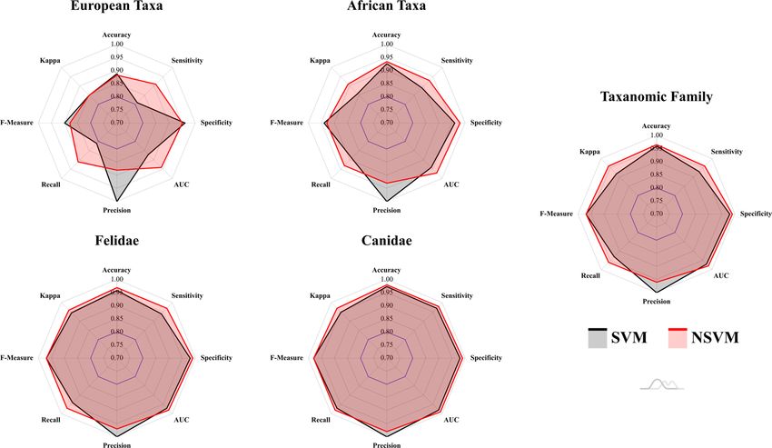
www.nature.com/scientificreports/
Figure 1. Variations in Form and Shape across tooth pits made by different taxa. (a) Variations in mean shape-
size relationships (top-view used for general morphology and front-view for depth). (b) Boxplot diagrams
representing centroid size distributions for each species (See Supplementary Table 1). (c) Mean landmark
configurations for carnivore tooth pits using Delaunay 2.5D Triangulation algorithms for mesh visualisations.
AfWD = Lycaon pictus. Figures created using the ggplot2 and scikit-learn Python and R libraries.
Modifications (BSM)17. This is especially relevant when considering techniques available for discerning of the
precise carnivore agencies involved in site formation processes.
Geometric Morphometrics (GM) are a popular multivariate statistical tool for the analysis of morphological
variance typically in biological s ystems18,19. Recent years, however, have seen an increase in GM applications
outside of anatomy. Applications in taphonomy have yielded impressive results when using GM as a tool for
morphological analyses and visualisation. From this perspective, multiple attempts have been made to use GM
as a diagnostic tool in carnivore taphonomy8,20–25. With the inclusion of Machine Learning (ML) algorithms, data
presented by Courtenay et al.20 present a promising advance for the integration of Artificial Intelligence (AI) and
advanced Data Science techniques with GM. Nevertheless, considering the relatively small sample size, these
results can also be considered optimistic. Likewise, in a recent study the original landmark model proposed24 was
found to present important margins of error product of landmark quality. These observations infer that analyst
experience condition the quality of r esults21.
Under this premise, the present study uses an updated version of the landmark model using semi-landmarks21,
and a much larger sample size to expand on the current referential samples available for taphonomic analyses.
These efforts aim to provide high quality data that can aid in the understanding of modern carnivore taxa that
are frequently found across Eurasia, Africa and the Americas. Samples include three types of felids (Panthera
leo, Panthera onca & Panthera pardus), three types of canids (Canis lupus, Vulpes vulpes & Lycaon pictus), the
spotted hyena (Crocuta crocuta), and the brown bear (Ursus arctos), that have been frequently subject of study
in Pleistocene research1,26–36. This larger sample allows us to conclude that > 90% separation of carnivore taxa is
still possible, with possibilities for even higher classification rates in the future.
Results
Geometric morphometrics. All samples are described by notable allometric patterns (Squared Residuals
= 0.006, F = 4.1, Effect Size = 2.7, p = 0.005, Bayes Factor Bound (BFB) = 13.88 against H0), indicating tooth pit
size to be an important conditioning factor in morphological variation. This is equally reflected when simply
considering Centroid Size values for each of the carnivores (Fig. 1, Table S1), with suggestive to strongly indica-
tive differences detected across most species (χ 2 = [5.08, 85.03], p < 0.007, BFB > 10.59). Exceptions to this
include C. crocuta, L. pictus and P. onca when these taxa are compared together (χ 2 = [0.14, 1.21], p > 0.27, BFB
< 1.04), as well as P. pardus when compared with C. lupus (χ 2 = 0.42, p = 0.51, BFB = 1.07 against Ha).
When considering multivariate morphological tendencies in form, general patterns reveal significant dif-
ferences throughout comparisons, with each of the taxonomic families being clearly separable (p ≈ 0.001, BFB
≈ 53.25). While the statistical separation was weakest when comparing Canidae and Ursidae (p = 0.003, BFB
= 21.11), as well as Ursidae and Hyaenidae (p = 0.006, BFB = 11.98), in both these cases differences remain of
notable interest ( p < 0.05). From a similar perspective, species within the families Canidae and Felidae appear
easily separable (p = 0.001, BFB = 53.25). When describing patterns of variation on a species-specific level, most
carnivores present statistical differences (p ≈ 0.001, BFB ≈ 53.26, Table S2 & S3), nevertheless, exceptions to
this can still be found. From this perspective, some degrees of equifinality are therefore still likely to exist when
Scientific Reports | (2021) 11:10209 | https://doi.org/10.1038/s41598-021-89518-4 2
Vol:.(1234567890)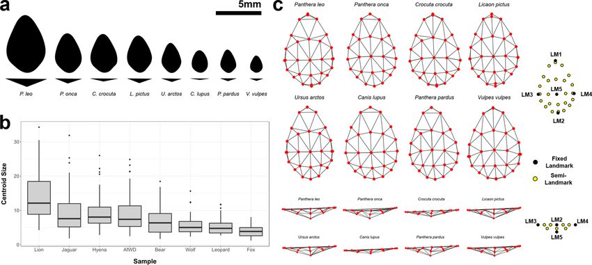
www.nature.com/scientificreports/

                                  Figure 2.  Anomaly detection results using Isolation Forests. Top Left Panel: Density of information within
                                  Principal Components Analysis. Top Right Panel: Distribution of Anomaly Scores; Vertical red line marks the
                                  acceptable threshold. Bottom Left Panel: Scatter plot heat map indicating the anomaly scores for each point.
                                  Bottom Right Panel: Final classifications of points as anomalies (True) or not (False). Figure created using the
                                  ggplot2 R library.

                                  comparing L. pictus, C. crocuta and P. onca (p > 0.8, BFB > 2.06 against Ha), as well as when comparing C. crocuta
                                  and P. onca (p = 0.17, BFB = 1.22).
                                      Exploring morphological variation through visualisations of mean landmark configurations reveal that the
                                  greatest differences appear when considering landmark displacements across the z-axis (Fig. 1). From this it can
                                  be seen that C. lupus tend to leave the most superficial traces, while P. leo leave some of the deepest and largest
                                  tooth pits of the entire sample. Interestingly, V. vulpes and L. pictus appear to leave very deep pits in relation to
                                  their size. Likewise, when considering variations across a horizontal plane (x and y axes), slight variations can
                                  be seen with some of the canids such as C. lupus and V. vulpes leaving more circular marks, while felids appear
                                  to leave more elongated pits (Fig. 1).
                                      When analysing these central morphological tendencies in accordance with taxonomic groupings, very weak
                                  phylogenetic signals are detected, indicating other confounding variables, such as biomechanics, exert a much
                                  stronger influence on tooth pit formation than cuspid morphology (Effect Size = − 0.99, p = 0.81, BFB = 2.16
                                  against Ha . Fig. S1).

                                  Unsupervised computational learning. Dimensionality reduction of datasets through Principal Com-
                                  ponents Analysis (PCA) produced high dimensional, non-homogeneously distributed and noisy datasets on
                                  all accounts. General analyses showed PCA in form space to produce a total of 90 Principal Component (PC)
                                  Scores, of which the first 6 PC Scores represent over 95% of the total sample variance. Analyses of optimal num-
                                  ber of components observed 5 PC scores to be the most representative. Nevertheless high residuals were still
                                  noted across a number of these dimensions.
                                      When preparing datasets for further processing, Isolation Forests (IF) proved effective for the elimination
                                  of anomalies across all 5 dimensions (Fig. 2). Nevertheless, a relatively high anomalous score threshold was
                                  needed for most anomaly detection tasks, considering how species like P. leo and C. lupus presented very high
                                  variability in comparison with other samples. This natural variability consequently produced a global increase
                                  of variance across all dimensions, frequently resulting in the adversarial effect of IFs over-classifying entire spe-
                                  cies as anomalies due to their abnormally large morphological variations. Under this premise, anomaly score
                                  distributions were allowed a slight positive tail, with thresholds in the present study defined between 0.625 and
                                  0.700. Using these thresholds, IFs were seen to remove between 3 and 10 pits for each dataset, with the most
                                  extreme removal of 10 pits occurring in the European Taxa dataset. Nevertheless, upon inspection of anomaly
                                  score distributions (Top right panel; Fig. 2), it can be argued that IFs were still able to preserve the majority of
                                  natural variability, only eliminating the most extreme of cases. In light of this, IFs were only seen to remove at
                                  most 2.3% of the original sample.
                                      Once datasets had been cleaned, data augmentation proved successful on all accounts with the generation of
                                  highly realistic synthetic data by both algorithms. Of the two algorithms tried and tested, Markov Chain Monte
                                  Carlo (MCMC, Fig. 3) algorithms appeared the fastest at generating new data with very high equivalency scores
                                  (Table 1). Experimentation found MCMCs to produce the most realistic data when sampling from robustly
                                  defined gaussian target distributions (|d| = 0.004, p = 1.2e−57, BFB = 2.3e+54), as opposed to the skewed-normal
                                  (|d| = 0.06, p = 1.3e−05, BFB = 2515). This was especially evident when considering the skewed-normal had the

Scientific Reports |   (2021) 11:10209 |               https://doi.org/10.1038/s41598-021-89518-4                                                    3

                                                                                                                                                Vol.:(0123456789)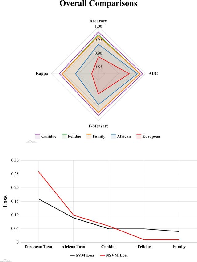
www.nature.com/scientificreports/

                                            Figure 3.  Example of trace figures, target density and histograms of the augmented and original datasets as
                                            generated using Markov Chain Monte Carlo algorithms. Figure created using the ggplot2 R library.

                                            tendency to exaggerate non-Gaussian elements, which may not be a true reflection of the population distribution
                                            (original skew = 0.18, augmented skew = 0.97).
                                                From the perspective of generative neural networks, of the three Generative Adversarial Networks (GANs),
                                            Wasserstein Gradient-Penalty loss GANs (WGAN-GP) produced the best results (|d| = 0.012, p = 2.4e−13, BFB
                                            = 5.3e+10). Nevertheless, while WGAN-GP proved successful on all datasets, the training of GAN models
                                            proved to be computationally expensive, with iterations taking ≈25,000 times longer than MCMC (χ 2 = 5.6, p
                                            = 0.018, BFB = 5.10).
                                                For final data augmentation tasks both MCMC and WGAN-GP were used, with the best performing algo-
                                            rithm being chosen to augment each dataset prior to supervised training (Tables 1, S4-7).

                                            Supervised computational learning. Both supervised models provided high accuracy in the classifica-
                                            tion of carnivore taxa (Tables 2 & S8-12, Figs. 4, 5 and 6), in most cases producing >90% accuracy (Area Under
                                            Curve (AUC) > 0.94, F-Measure > 0.93, κ > 0.86). The only exception to this can be found in the case of the
                                            Pleistocene European Taxa dataset, which only produced >85% accuracy (AUC ≈ 0.90, F ≈ 0.89, κ ≈ 0.85). Upon
                                            analysing the overall performance of each dataset, the greatest results are obtained when differentiating between
                                            taxonomic families (Accuracy > 96%, AUC > 0.97, F > 0.97, κ > 0.92), as well as the specific species within these
                                            families (Table S11 & S12). This can be seen in the cases of the Canidae (Acc. > 97%, AUC > 0.98, F > 0.98, κ >
                                            0.95), and the Felidae datasets (Acc. > 96%, AUC > 0.97, F > 0.97, κ > 0.95).
                                                When pooling many labels, especially with taxa from different families, overall classification rates tend to
                                            drop. Nevertheless, while classification rates may fall below 90% accuracy, miss-classification rates and the fre-
                                            quency of Type I and Type II errors do not rise above 0.2 when considering overall performance (Fig. 4), resulting
                                            in very high AUC, Kappa and F scores as well. Under this premise, both Support Vector Machines (SVM) and
                                            Neural SVMs (NSVM) can be considered highly efficient classifiers of carnivore tooth marks, yet with greater
                                            performance when working with a smaller number of labels. Needless to say, when considering loss values, with
                                            the exception of the Pleistocene European dataset, both SVM and NSVM appear to be confident when making
                                            new predicitons (Fig. 6).
                                                By considering model performance on individual samples (Tables S8-S12), differentiating between taxa
                                            appears to depend on the species being used for comparison. Under this premise, V. vulpes (Tables S8) and P. leo
                                            (Tables S9) appear to be the easiest of the Pleistocene European and African carnivores to identify (SVM Acc. =
                                            {95%, 95%}, NSVM Acc. = {94%, 96%}, respectively). On the scale of taxonomic families, L. pictus can be con-
                                            sidered the easiest canid to identify (SVM Acc. = 98%, NSVM Acc. = 100%), while P. leo remains the felid with
                                            the highest classification rates (SVM Acc. = 96%, NSVM Acc. = 99%). Each of these observations are especially

          Scientific Reports |   (2021) 11:10209 |               https://doi.org/10.1038/s41598-021-89518-4                                                 4

Vol:.(1234567890)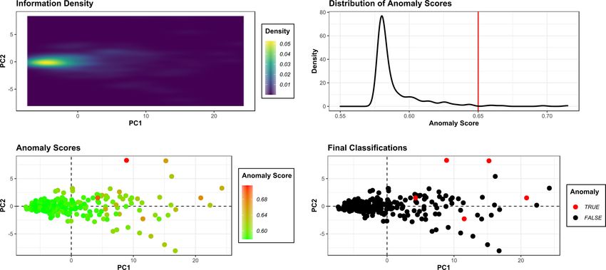
www.nature.com/scientificreports/
Algorithm Animal Measure PC1 PC2 PC3 PC4 PC5 Time (Ms)
|d| 0.007 0.011 0.016 0.115 0.037
C. crocuta p 4.9e−13 2.7e−09 6.8e−16 1.3e−08 8.9e−22 1311
BFB 2.6e+10 6.9e+06 1.5e+13 1.6e+06 8.5e+18
|d| 0.092 0.010 0.022 0.007 0.016
P. pardus p 3.4e−18 3.6e−37 2.9e−32 1.5e−36 1.4e−36 1194
BFB 2.7e+15 1.2e+34 1.7e+29 3.0e+33 3.2e+33
WGAN-GP
|d| 0.034 0.009 0.046 0.001 0.004
L. pictus p 1.2e−08 1.0e−12 1.4e−19 4.8e−33 4.0e−16 1296
BFB 1.7e+06 1.3e+10 6.1e+16 1.0e+30 2.6e+13
|d| 0.097 0.005 0.008 0.043 0.003
P. leo p 6.3e−03 5.5e−10 5.8e−10 1.5e−08 1.6e−15 915
BFB 11.52 3.1e+07 3.0e+07 1.4e+06 6.7e+12
|d| 0.055 0.010 0.010 0.004 0.003
C. crocuta p 5.8e−13 4.3e−40 8.5e−73 6.0e−63 3.6e−62 0.048
BFB 2.3e+10 9.4e+36 2.6e+69 4.3e+59 7.2e+58
|d| 0.004 0.007 0.004 0.003 0.007
P. pardus p 6.9e−29 4.8e−70 1.5e−104 2.8e−75 1.0e−85 0.048
BFB 8.2e+25 4.8e+66 1.0e+101 7.7e+71 1.9e+82
MCMC
|d| 0.007 0.010 0.003 0.004 0.003
L . pictus p 9.6e−12 3.3e−42 4.5e−83 1.7e−67 2.5e−57 0.047
BFB 1.5e+09 1.2e+39 4.3e+79 1.4e+64 1.1e+54
|d| 0.023 0.010 0.002 0.004 0.001
P. leo p 1.1e−05 1.0e−32 3.4e−54 8.6e−39 1.5e−50 0.048
BFB 2.9e+03 5.0e+29 8.8e+50 4.9+e35 2.1e+47
Table 1. Examples of absolute difference (|d|), p-Values and Bayes Factor Bounds (BFB) obtained when
assessing the robust equivalency of synthetic data and real data using Gradient Penalty Wasserstein Loss
Generative Adversarial Networks (WGAN-GP) and Markov Chain Monte Carlo (MCMC) Algorithms for
data augmentation of the African Taxa dataset. Time values reported represent the number of miliseconds per
epoch or iteration of the algorithm.
Sample Algorithm Acc. Sens. Spec. Prec. Rec. AUC F κ Loss
SVM 0.89 0.81 0.96 1.00 0.81 0.87 0.90 0.85 0.16
Pleistocene European Taxa
NSVM 0.88 0.91 0.95 0.88 0.91 0.94 0.88 0.85 0.26
SVM 0.93 0.89 0.96 1.00 0.89 0.94 0.94 0.86 0.09
African Taxa
NSVM 0.93 0.93 0.98 0.93 0.93 0.97 0.93 0.91 0.10
SVM 0.96 0.93 0.98 1.00 0.93 0.97 0.97 0.92 0.05
Taxonomic family
NSVM 0.97 0.96 0.99 0.96 0.96 0.98 0.97 0.96 0.06
SVM 0.97 0.97 0.98 1.00 0.97 0.98 0.98 0.95 0.05
Canidae
NSVM 0.98 0.98 0.99 0.98 0.98 0.99 0.98 0.97 0.01
SVM 0.96 0.94 0.98 1.00 0.94 0.97 0.97 0.95 0.04
Felidae
NSVM 0.97 0.97 0.99 0.97 0.97 0.98 0.97 0.96 0.01
Table 2. Overall classification results obtained for all samples using Support Vector Machines (SVM) and
Neural Support Vector Machines (NSVM). Reported values include; Accuracy (Acc.), Sensitivity (Sens.),
Specificity (Spec.), Precision (Prec.), Recall (Rec.), Area Under Curve (AUC), F-Measure (F), Kappa (κ) and
Loss. All evaluation metrics (with the exception of loss) are recorded as values between 0 and 1, with 1 being
the highest obtainable value. Values reported over 0.8 are considered an acceptable threshold for powerful
classification models. Loss considers values closer to 0 as the most confident models.
interesting considering these species have been associated with either the largest or the smallest centroid sizes
respectively (Fig. 1, Table S1).
While P. pardus presents the lowest recorded individual classification rates across all datasets (NSVM Acc. =
0.79, Table S8), this does not have a significant impact on overall model performance (Fig. 4). Even when con-
sidering the poorer classification rates presented by P. pardus, all algorithms achieve evaluation metrics above
Scientific Reports | (2021) 11:10209 | https://doi.org/10.1038/s41598-021-89518-4 5
Vol.:(0123456789)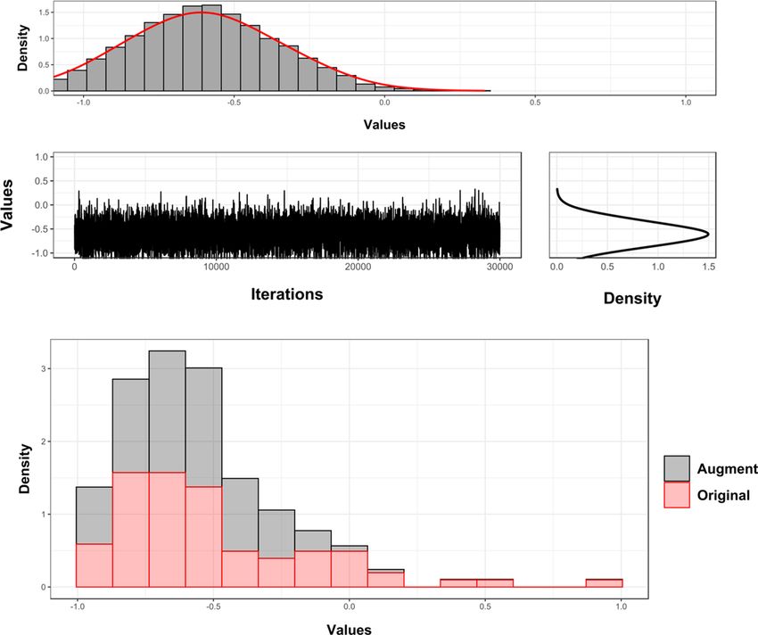
www.nature.com/scientificreports/
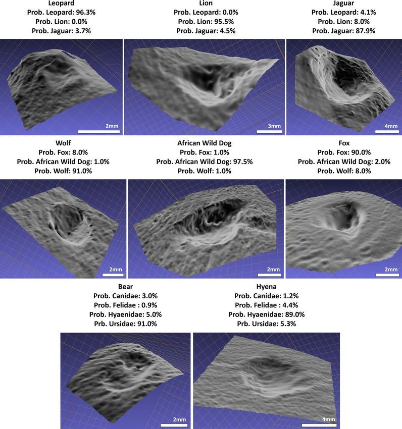
Figure 4. Radar plots representing supervised classification results for each of the datasets. Evaluation
metrics were calculated on test sets when using both Support Vector Machines (SVM) and Neural Support
Vector Machines (NSVM). The blue line marking 0.8 across all graphs represents a standard threshold for the
evaluation of good performance for each of the metrics used. Figure created using the amCharts4 JavaScript
library.
the acceptable 0.8 threshold. Likewise, a 97% to 99% accuracy has still been obtained when comparing P. pardus
with other felids (Fig. 5), and a 92% to 93% accuracy when compared with other African species.
Although an element of equifinality is still present, as detected through inconclusive statistical differences in
some tooth pit morphologies, both SVM and NSVM are still able to accurately differentiate between L. pictus
and C. crocuta with over 90% success. Nevertheless, algorithm confidence when performing classifications on
these species drops, as seen through a large increase in loss values (Table S9). This results in the overall rise in
loss and decrease in other performance metrics when these two species are included in a dataset (Table 2, Fig. 6).
Observations comparing SVM with NSVM prove both algorithms to be equally powerful when discerning
between carnivore taxa. While NSVM may be seen to have a slight advantage over SVM in some evaluation
metrics (Fig. 4), SVM loss rates are generally lower (Fig. 6). Similiarly, NSVM can be seen in some datasets to
have very low loss rates for some groups (e.g. Table S10, Canidae loss = 0.001), while especially high loss rates
for others (e.g. Table S10, Hyaenidae loss = 0.19). In sum, both SVM and NSVM are valid options for carnivore
differentiation, while choice of one or the other must be dependent on the specific case study at hand as well as
the analyst’s needs.
When observing general performance in model loss (Fig. 6), algorithms produce powerful predictions, with
very confident decision boundaries in many cases (Fig. 5).
Finally, when training algorithms without the use of data augmentation (Sup. Appendix 7), it can be seen
how the average accuracy slightly drops, with SVM performing 4% worse on non-augmented datasets and
NSVM performing 6% worse. While this change is minute, the greatest differences between augmented and
non-augmented datasets can be found across loss values, with both SVM and NSVM loosing an average of
10% confidence with each prediction made. As would be expected, algorithms also appear to perform worse on
unbalanced datasets, with the Taxonomic Family dataset presenting F-Measure values 0.25 lower, especially in
the case of NSVM (Sup. Appendix 7).
Discussion
In recent years, GM have been applied to a wide array of different applications outside of biology. Among these
applications, these tools have shown promising results when applied to the study of B SMs8,20–25,37. While subse-
quent analyses have identified some issues with these techniques for carnivore BSM applications21, the present
study has shown that high quality results are still realistically obtainable (Accuracy > 90 %, AUC > 0.8, κ > 0.8,
Fig. 6). Likewise, the results reported here are supported by considerably larger sample sizes20,22,24.
Here we have shown how a number of different data science tools can be employed for GM analyses. From one
perspective, unsupervised computational learning approaches were able to produce highly realistic augmented
Scientific Reports | (2021) 11:10209 | https://doi.org/10.1038/s41598-021-89518-4 6
Vol:.(1234567890)www.nature.com/scientificreports/
Figure 5. Example of tooth pit classifications using Neural Support Vector Machines (NSVM). The select tooth
pits were chosen randomly and excluded from the training data so as to avoid bias. NSVMs were then trained
on the remaining data and used to classify the present tooth marks, taking note of the algorithms confidence
when making predictions. 3D visualisations were created using MeshLab.
datasets, using both neural network based a pproaches38–41, as well as Bayesian Inference E ngines42–45. While the
use of Graphics Processing Units (GPUs) are likely to speed up GAN performance, MCMC can still be consid-
ered the fastest approach to modelling these datasets with exceptional synthetic-data quality. From a Bayesian
perspective, considering how the use of Gaussian distributions is usually seen as a “crude approximation” to the
problem solving questions at h and45, most of the times this also allows models greater generalization capabili-
ties. In addition, this theoretically reduces chance of overfitting supervised models on one particular skewed
distribution that may not be a true reflection of the population distribution (Sup. Appendix 4). Moreover, to
ensure the present study does not fall into the trap of over-generalising the Gaussian nature of the population,
the precise definitions of our target probability distributions were robustly defined41,46,47.
Scientific Reports | (2021) 11:10209 | https://doi.org/10.1038/s41598-021-89518-4 7
Vol.:(0123456789)www.nature.com/scientificreports/
Figure 6. Top Panel: Radar plot summarising and comparing performance of the best computational learning
models for each of the datasets. Bottom panel: Line graph representing the mean reported loss for both Support
Vector Machines (SVM) and Neural Support Vector Machines (NSVM) on each of the datasets. Figure created
using the amCharts4 JavaScript library.
From the perspective of supervised learning, the present study reveals the capabilities of computational learn-
ing algorithms for the differentiation of carnivore taxa based on the morphology of carnivore tooth pits. Firstly,
prior augmentation of each dataset provided both algorithms with enough information to learn from, obtaining
above average accuracy when used to classify the original samples. While the present datasets are unable to reach
the 100% accuracy reported originally using SVMs20, this is likely due to the use of bootstrapping in the original
study41. Here, more robust data augmentation techniques produced completely new synthetic data from which
to learn from, providing a more general overview of the target domain. Under this premise, while 100% accu-
racy was not obtained, our reported >90% can be considered much more reliable. From a similar perspective,
while the changes to the original landmark model have shown a reduction in inter-analyst error by 164µm21, the
inclusion of semi-landmark patches has been observed to substantially increase the dimensionality of these GM
datasets. In light of this, the new datasets are likely to be harder to model from. Needless to say, considering the
increased precision of the landmark model, alongside more robust augmentation techniques, it can be argued
that the present results are not only more reliable, but also worth the slight drop in accuracy.
Despite the increase in landmark model complexity, both Radial kernel functions and Laplacian fourier
mappings were able to provide SVMs with an appropriate transformed feature space to learn from. Neverthe-
less, both SVM and NSVM have their advantages and disadvantages. NSVM, for example, can be considered a
complex model, with the additional requirement of fine tuning a neural network architecture for feature map-
pings. NSVM thus presents a large number of parameters and hyperparametrs that have to be adjusted by both
the analyst and the model itself. SVM, on the other hand, has the distinct advantage of being easier to tune and
train, yet, when using Bayesian algorithms for SVM hyperparameter optimization, training time can increase
significantly (Table S13), while NSVMs still perform better on some datasets.
From the perspective of combining supervised and unsupervised learning approaches, the present study can
be considered another example of how powerful data augmentation can be for improving classification model
performance. Data augmentation is a very popular technique in computer vision, nevertheless, not all of these
algorithms are readily applicable to numeric data of this t ype48. Here augmentation has been shown to not only
improve the accuracy of most models (Tables 2, S8-S12 & S23-S28, Supplementary Appendix 7), but also improve
the generalization capabilities of both SVMs and N SVMs41,49. This is mostly seen through the decrease in loss
values across taxa (Tables S8-S12 & S23-S28), thus supporting observations made by Courtenay and González-
Aguilera41 when applied to other GM datasets of palaeoanthropological and primatological origin. Similarly,
the impact dataset imbalance has on algorithm performance is clearly evident, as seen through great drops in
Scientific Reports | (2021) 11:10209 | https://doi.org/10.1038/s41598-021-89518-4 8
Vol:.(1234567890)www.nature.com/scientificreports/
precision, recall and F values (Supplementary Appendix 6, Tables S8-S12 & S23-S28). In light of each of these
observations, it can be seen how data augmentation can be a valuable tool for archaeological and palaeontological
applications41, especially in cases where obtaining large sample sizes is difficult.
In the general context of new technologies applied to the field of taphonomy, it can be noted how the inclusion
of some carnivore species within the samples have created notable statistical noise. This can be seen through drops
in performance when increasing the number of target labels used in classification (e.g. the Pleistocene European
Taxa dataset). From this perspective, it is important to point out that highly sophisticated techniques are not the
all-encompassing solution that many analysts are looking for. When considering how carnivores can usually
be described by the t ype2,3,30, ratio27,34,36,50 and size of bite d
amage51–53, alongside the location54–56 and extent of
damage57, it can be seen how modelling carnivore behaviour should also take into account a wide range of dif-
ferent factors beyond BSMs. While neither one of these techniques can exclusively answer these questions, when
combined, taphonomists currently have a very powerful toolkit at their disposal for discerning precise carnivore
intervention. From a similar perspective, techniques in remote sensing, photogrammetry and microscopy also
provide distinct advantages for the collection of different types of data, supported in many cases by the use of
high resolution metric d ata37,58–60. Likewise, the use of computational learning has also proven a useful diagnostic
tool for the analysis of fracture plane patterns61, obtaining high classification rates when applied to archaeological
samples as well62. From another perspective, computer vision applications can also be considered an interesting
development in the field of taphonomy63. In sum, and wherever possible, rather than commingling multiple spe-
cies together into one large group, prior processes of elimination based on general taphonomic evidence should
be performed in order to remove the least likely animals to have intervened. Algorithms will then be much easier
to train, obtaining state of the art classification rates.
“Occam’s Razor” suggests that a more complex model is not always a better one. As seen here, without the
use of large kernel machines, SVMs are equally likely to produce high level results. Likewise, while GANs are
powerful non-parametric generative models, Bayesian inference is still a valuable tool for distribution model-
ling, as seen through better and faster performance in some of the reported cases. From this perspective, data
science applications and AI can be considered both a very promising field of research, as well as a complex and
challenging “pandoras box” of algorithms which analysts must take into consideration before planning a study.
Nevertheless, and in combination with multiple other sources of data, advanced data science techniques can be
considered a significant contribution to a taphonomist’s arsenal.
Material and methods
Sample. A total of 620 carnivore tooth pits were included in the present study. These samples included tooth
marks produced by;
• Brown Bears (Ursus arctos, Ursidae, 69 pits)
• Spotted Hyenas (Crocuta crocuta, Hyaenidae, 86 pits)
• Wolves (Canis lupus, Canidae, 80 pits)
• African Wild Dogs (Lycaon pictus, Canidae, 89 pits)
• Foxes (Vulpes vulpes, Canidae, 53 pits)
• Jaguars (Panthera onca, Felidae, 77 pits)
• Leopards (Panthera pardus, Felidae, 84 pits)
• Lions (Panthera leo, Felidae, 82 pits)
Samples originated from a number of different sources, including animals kept in parks as well as wild animals.
Samples obtained from wild animals included those produced by foxes as well as wolves. The only sample contain-
ing both wild and captive animals was the wolf sample. Preliminary data from these tooth pits revealed animals
in captivity to have highly equivalent tooth pit morphologies to wild animals (|d| = 0.125, p = 9.0e−14, BFB =
1.4e+11), while tooth scores revealed otherwise (|d| = 0.152, p = 0.99, BFB = 3.7e+01 against Ha ). Under this
premise, and so as to avoid the influence of confounding variables that go beyond the scope of the present study,
tooth scores were excluded from the present samples and are under current investigation (data in preperation).
Nevertheless, other research have shown tooth pits to be more informative than tooth scores when considering
morphology20,23.
When working with tooth mark morphologies, preference is usually given to marks found on long bone
diaphyses. This is preferred considering how diaphyses are denser than epiphyses, and are thus more likely to
survive during carnivore feeding. Nevertheless, when working with captive or semi-captive animals, controlling
the bones that carnivores are fed is not always possible. This is due to the rules and regulations established by the
institution where these animals are k ept64. While this was not an issue for the majority of the animals used within
the present study, in the case of P. pardus, animals were only fed ribs in articulation with other axial elements.
In light of this, a careful evaluation on the effects this may have on the analogy of our samples was performed
(Supplementary Appendix 2). These reflections concluded that in order to maintain a plausible analogy with
tooth marks produced by other animals on diaphyses, tooth marks could only be used if found on the shaft of
bovine ribs closest to the tuburcle, coinciding with the posterior and posterior-lateral portions of the rib, and
farthest away from the costochondral junction65. This area of the rib corresponds to label RI3 described by Lam
et al.65. Moreover, with a reported average cortical thickness of 2.3mm (± 0.13 mm) and Bone Mineral Density
of 4490kg/m3 [213.5, 334.6]66, bovine ribs are frequently employed in most bone simulation experiments used in
agricultural as well as general surgical sciences. Finally, considering the grease, muscle and fat content of typi-
cal domestic bovine individuals67, alongside the general size of P. pardus teeth, it was concluded that the use of
rib elements for this sample was the closest possible analogy to the tooth marks collected from other animals.
Scientific Reports | (2021) 11:10209 | https://doi.org/10.1038/s41598-021-89518-4 9
Vol.:(0123456789)www.nature.com/scientificreports/
Carnivores were fed a number of different sized animals, also dependent in most cases on the regulations
established by the institution where these animals are k ept64. Nevertheless, recent research has found statistical
similarities between tooth marks found on different a nimals25, with the greatest differences occurring between
large and small sized animals. Needless to say, considering the typical size of prey some of these carnivores
typically consume, this factor was not considered of notable importance for the present s tudy25 (Supplementary
Appendix 1).
For the purpose of comparisons, animals were split into 5 groups according to ecosystem as well as taxonomic
family. From an ecological perspective, two datasets were defined; (1) the Pleistocene European Taxa dataset con-
taining U. arctos, V. vulpes, C. crocuta, P. pardus, P. leo and C. lupus; and (2) the African Taxa dataset containing
C. crocuta, P. pardus, L. pictus and P. leo. When considering taxonomic groupings, animals were separated into
3 groups, including; (1) the Canidae dataset, including V. vulpes, L. pictus and C. lupus; (2) the Felidae dataset,
including P. pardus, P. onca and P. leo; and (3) a general Taxonomic Family dataset, including all Canidae in the
same group, all Felidae in the same group, followed by Hyaenidae and Ursidae. Some complementary details on
each of these carnivores have been included in Supplementary Appendix 1.
All experiments involving carnivores were performed in accordance with the relevant ethical guidelines as
set forth by park keepers and general park regulations. No animals were sacrificed specifically for the purpose
of these experiments. Likewise, carnivores were not manipulated or handled at any point during the collection
of samples. Collection of chewed bones were performed directly by park staff and assisted by one of the authors
(JY). The present study followed the guidelines set forth by ARRIVE (https://arriveguidelines.org/) wherever
necessary. No licenses or permits were required in order to perform these experiments. Finally, in the case of
animals in parks, bone samples were provided by the park according to normal feeding protocols. More details
can be consulted in the Extended Samples section of the supplementary files.
3D modelling and landmark digitisation. Digital reconstructions of tooth marks were performed using
Structured Light Surface Scanning (SLSS)68. The equipment used in the present study was the DAVID SLS-2
Structured Light Surface Scanner located in the C.A.I. Archaeometry and Archaeological Analysis lab of the
Complutense University of Madrid (Spain). This equipment consists of a DAVID USB CMOS Monochrome
2-Megapixel camera and ACER K11 LED projector. Both the camera and the projector were connected to a
portable ASUS X550VX personal laptop (8 GB RAM, I ntel® CoreTM i5 6300HQ CPU (2.3 GHz), NVIDIA GTX
950 GPU) via USB and HDMI respectively. The DAVID’s Laser Scanner Professional Edition software is stored
in a USB Flash Drive. Equipment were calibrated using a 15 mm markerboard, using additional macro lenses
attached to both the projector and the camera in order to obtain optimal resolution at this scale. Once calibrated
the DAVID SLS-2 produces a point cloud density of up to 1.2 million points which can be exported for further
processing via external software.
The landmark configuration used for this study consists of a total of 30 landmarks (LMs)21; 5 fixed Type II
landmarks18 and a 5 × 5 patch of semilandmarks69 (Fig. S2). Of the 5 fixed landmarks, LM1 and LM2 mark the
maximal length (l) of each pit. For the correct orientation of the pit, LM1 can be considered to be the point along
the maximum length furthest away from the perpendicular axis marking the maximum width (w). LM2 would
therefore be the point closest to said perpendicular axis (see variables d1 and d2 in Fig. S2 for clarification). LM3
and LM4 mark the extremities of the perpendicular axis (w) with LM3 being the left-most extremity and LM4
being the right-most extremity. LM5 is the deepest point of the pit. The semilandmark patch is then positioned
over the entirety of the pit, so as to capture the internal morphology of the mark.
Landmark collection was performed using the free Landmark Editor software (v.3.0.0.6.) by a single expe-
rienced analyst. Inter-analyst experiments prior to landmark collection revealed the landmark model to have
a robustly defined human-induced margin of error of 0.14 ± 0.09 mm (Median ± Square Root of the Biweight
Midvariance). Detailed explanations as well as an instructional video on how to place both landmarks and sem-
ilandmarks can be consulted in the Supplementary Appendix and main text of Courtenay et al.21.
Geometric morphometrics. Once collected, landmarks were formatted as morphologika files and
imported into the R free software environment (v.3.5.3, https://www.r-project.org/). Initial processing of these
files consisted in the orthogonal tangent projection into a new normalized feature space. This process, frequently
referred to as Generalized Procrustes Analysis (GPA), is a valuable tool that allows for the direct comparison
of landmark configurations18,19,70. GPA utilises different superimposition procedures (translation, rotation and
scaling) to quantify minute displacements of individual landmarks in s pace71. This in turn facilitates the com-
parison of landmark configurations, as well as hypothesis testing, using multivariate statistical analyses. Never-
theless, considering observations made by Courtenay et al.20,21,25 revealed tooth mark size to be an important
conditioning factor in their morphology, prior analyses in allometry were also performed72. From this perspec-
tive, allometric analyses first considered the calculation of centroid sizes across all individuals; the square root of
the sum of squared distances of all landmarks of an object from their centroid18. These calculations were then fol-
lowed by multiple regressions to assess the significance of shape-size relationships. For regression, the logarithm
of centroid sizes were used. In cases where shape-size relationships proved significant, final superimposition
procedures were performed excluding the scaling step of GPA (form).
In addition to these analyses, preliminary tests were performed to check for the strength of phylogenetic
signals73. This was used as a means of testing whether groups of carnivores produced similar tooth pits to other
members of the same taxonomic family. For details on the phylogenies used during these tests, consult Fig. S1
and Supplementary Appendix 1.
For the visualisation of morphological trends and variations, Thin Plate Splines (TPS) and central morpho-
logical tendencies were calculated19,71. From each of these mean landmark configurations, for ease of pattern
Scientific Reports | (2021) 11:10209 | https://doi.org/10.1038/s41598-021-89518-4 10
Vol:.(1234567890)www.nature.com/scientificreports/
visualisation across so many landmarks, final calculations were performed using Delaunay 2.5D Triangulation
algorithms74 creating visual meshes of these configurations in Python (v.3.7.4, https://www.python.org/).
Once normalised, landmark coordinates were processed using dimensionality reduction via Principal Com-
ponents Analyses (PCA). In order to identify the optimal number of Principal Component Scores (PC Scores)
that best represented morphological variance, permutation tests were performed calculating the observed vari-
ance explained by each PC with the permuted variance over 50 randomized iterations75. Multivariate Analysis
of Variance (MANOVA) tests were then performed on these select PCs to assess the significance of multivariate
morphological variance among samples.
Geometric Morphometric applications were programmed in the R programming language (Sup. Appendix 8).
Robust statistics. While GPA is known to normalize data76, this does not always hold true. Under this
premise, caution must be taken when performing statistical analyses on these datasets. Taking this into consid-
eration, prior to all hypothesis testing, normality tests were also performed. These included Shapiro tests and
the inspection of Quantile–Quantile graphs. In cases where normality was detected, univariate hypothesis tests
were performed using traditional parametric Analysis of Variance (ANOVA). For multivariate tests, such as
MANOVA, calculations were derived using the Hotelling-Lawley test-statistic. When normality was rejected,
robust alternatives to each of these tests were chosen. In the case of univariate testing, the Kruskal–Wallis non-
parametric rank test was prefered, while for MANOVA calculations, Wilk’s Lambda was used.
Finally, in light of some of the recommendations presented by The American Statistical Association (ASA), as
debated in Volume 73, Issue Sup1 of The American Statistician77,78, the present study considers p-values of > 2σ
from the mean to indicate only suggestive support for the alternative hypothesis ( Ha ). p > 0.005, or where
possible, 3σ was therefore used as a threshold to conclude that Ha is “significant”. In addition, Bayes Factor Bound
(BFB) values (Eq. 1) have also been included alongside all corresponding p-Values79. Unless stated otherwise,
BFBs are reported as the odds in favor of the alternative hypothesis (BFB:1). More details on BFB, Bayes Fac-
tors and the p > 3σ threshold have been included in Supplementary Appendix 3. General BFB calibrations in
accordance with Benjamin and Berger’s Recommendation 0.379, as well as False Positive Risk values according
to Colquhoun’s p roposals80, have also been included in Table S20 of Supplementary Appendix 3.
1
BFB = (1)
−e p log(p)
All statistical applications were programmed in the R programming language (Sup. Appendix 8).
Computational learning. Computational Learning employed in this study consisted of two main types
of algorithm; Unsupervised and Supervised algorithms. The concept of “learning” in AI refers primarily to the
creation of algorithms that are able to extract patterns from raw data (i.e. “learn”), based on their “experience”
through the construction of mathematical functions38,81. The basis of all AI learning activities include the com-
bination of multiple components, including; linear algebra, calculus, probability theory and statistics. From this,
algorithms can create complex mathematical functions using many simpler concepts as building b locks38. Here
we use the term “Computational Learning” to refer to a very large group of sub-disciplines and sub-sub-disci-
plines within AI. Deep Learning and Machine Learning are terms frequently used (and often debated), however,
many more branches and types of learning exist. Under this premise, and so as to avoid complication, the present
study has chosen to summarise these algorithms using the term “Computational”.
Similar to the concepts of Deep and Machine Learning, many different types of supervision exist. The terms
supervised and unsupervised refer to the way raw data is fed into the algorithm. In most literature, data will
be referred to via the algebraic symbol x, whether this be a vector, scalar or matrix. The objective of algorithms
are to find patterns among a group of x. In an unsupervised context, x is directly fed into the algorithm without
further explanation. Algorithms are then forced to search for patterns that best explain the data. In the case of
supervised contexts, x is associated with a label or target usually denominated as y. Here the algorithm
will try
and find the best means of mapping x to y. From a statistical perspective, this can be explained as p y|x . In sum,
unsupervised algorithms are typically used for clustering tasks, dimensionality reduction or anomaly detection,
while supervised learning is typically associated with classification tasks or regression.
The workflow used in the present study begins with dimensionality reduction, as explained earlier with the
use of PCA. While preliminary experiments were performed using non-linear dimensionality reduction algo-
rithms, such as t-distributed Stochastic Neighbor Embedding (t-SNE)82 and Uniform Manifold Approximation
and Projection (UMAP)83, PCA was found to be the most consistent across all datasets, a point which should be
developed in detailed further research. Once dimensionality reduction had been performed, and prior to any
advanced computational modelling, datasets were cleaned using unsupervised Isolation Forests (IFs)84. Once
anomalies had been removed, data augmentation was performed using two different unsupervised approaches;
Generative Adversarial Networks (GANs)38–41 and Markov Chain Monte Carlo (MCMC) s ampling44. Data aug-
mentation was performed for two primary reasons; (1) the simulation of larger datasets to ensure supervised
algorithms have enough information to train from, and (2) to balance datasets so each sample has the same size.
Both MCMCs and GANs were trialed and tested using robust statistics to evaluate quality of augmented d ata41.
Once the best model had been determined, each of the datasets were augmented so they had a total sample size
of n = 100. In the case of the Taxonomic Family dataset, augmentation was performed until all samples had the
same size as the largest sample.
Once augmented, samples were used for the training of supervised classification models. Two classifica-
tion models were tried and tested; Support Vector Machines (SVM)85 and Neural Support Vector Machines
(NSVM)86,87. NSVMs are an extension of SVM using Neural Networks (NNs)38 as feature extractors, in
Scientific Reports | (2021) 11:10209 | https://doi.org/10.1038/s41598-021-89518-4 11
Vol.:(0123456789)www.nature.com/scientificreports/
substituting the kernel functions typically used in SVMs. Hyperparameter optimization for both SVMs and
NSVMs were performed using Bayesian Optimization Algorithms (BOAs)88.
Supervised computational applications were performed in both the R and Python programming languages
(Sup. Appendix 8). For full details on both unsupervised and supervised computational algorithms, consult the
Extended Methods section of the Supplementary Materials.
Evaluation of supervised learning algorithms took into account a wide array of different popular evaluation
metrics in machine and deep learning. These included; Accuracy, Sensitivity, Specificity, Precision, Recall, Area
Under the receiver operator characteristic Curve (AUC), the F-Measure (also known as the F1 Score), Cohen’s
Kappa (κ) statistic, and model Loss. Each of these metrics, with the exception of loss, are calculated using confu-
sion matrices, measuring the ratio of correctly classified individuals (True Positive & True Negative) as well as
miss-classified individuals (False Positive & False Negative). For more details see Supplementary Appendix 6.
Accuracy is simply reported as either a decimal [0, 1] or a percentage. Accuracy is a metric often misinter-
preted, as explained in Supplementary Appendix 6, and should always be considered in combination with other
values, such as Sensitivity or Specificity. Both Sensitivity and Specificity are values reported as decimals [0, 1],
and are used to evaluate the proportion of correct classifications and miss-classifications. AUC values are derived
from receiver operator characteristic curves, a method used to balance and graphically represent the rate of cor-
rectly and incorrectly classified individuals. The closest the curve gets to reaching the top left corner of the graph,
the better the classifier, while diagonal lines in the graph represent a random classifier (poor model). In order
to quantify the curvature of the graph, the area under the curve can be calculated (AUC), with AUC = 1 being
a perfect classifier and AUC = 0.5 being a random classifier. The κ statistic is a measure of observer reliability,
usually employed to test the agreement between two systems. When applied to confusion matrix evaluations, κ
can be used to assess the probability that a model will produce an output ŷ that coincides with the real output y.
κ values typically range between [0, 1], with κ = 1 meaning perfect agreement, κ = 0 being random agreement,
and κ = 0.8 typically used as a threshold to define a near-perfect or perfect algorithm.
While in the authors’ opinion, AUC, Sensitivity and Specificity values are the most reliable evaluation metrics
for studies of this type (Supp. Appendix 6), for ease of comparison with other papers or authors who choose to
use other metrics, we have also included Precision, Recall and F-Measure values. Precision and Recall values
play a similar role to sensitivity and specificity, with recall being equivalent to sensitivity, and precision being the
calculation of the number of correct positive predictions made. Precision and Recall, however, differ from their
counterparts in being more robust to imbalance in datasets. F-Measures are a combined evaluation of these two
measures. For more details consult Supplementary Appendix 6.
Loss metrics were reported using the Mean Squared Error (Eq. 2);
n
1
2
MSE = yi − ŷi (2)
n
i=1
Loss values are interpreted considering values closest to 0 as an indicator of greater confidence when using
the model to make new predictions.
Final evaluation metrics were reported when using algorithms to classify only the original samples, without
augmented data. Augmented data was, therefore, solely used for training and validation. Finally, so as to assess
the impact data augmentation has on supervised learning algorithms, algorithms were also trained on the raw
data. This was performed using 70% of the raw data for training, while the remaining 30% was used as a test set.
Data availability
All the relevant data and code used for the present study have been made readily available online via the cor-
responding author’s GitHub page: https://github.com/LACourtenay/Carnivore_Tooth_Pit_Classification. Any
queries or issues regarding data or code should be directed to L.A. Courtenay (ladc1995@gmail.com).
Received: 16 February 2021; Accepted: 27 April 2021
References
1. Brain, C. K. Hunters or the Hunted? An introduction to African cave taphonomy (University of Chicago Press, 1981).
2. Binford, L. R. Bones: Ancient Men and Modern Myths (Academic Press Inc., 1981).
3. Blumenschine, R. Percussion marks, tooth marks and experimental determinations of the timing of hominid and carnivore access
to long bones at FLK Zinjanthropus, Olduvai Gorge, Tanzania. J. Hum. Evol. 29(1), 21–51 (1995).
4. Domínguez-Rodrigo, M., Barba, R. & Egeland, C. P. Deconstructing Olduvai (Springer, 2007).
5. Andrews, P. & Fernandez-Jalvo, Y. Surface modifications of the Sima de los Huesos fossil humans. J. Hum. Evol. 33, 191–217 (1997).
6. Cueto, M., Camarós, E., Castaños, P., Ontañón, R. & Arias, P. Under the skin of a lion: unique evidence of Upper Paleolithic
exploitation and use of cave lion (Panthera spelaea) from the Lower Gallery of La Garma (Spain). PLoS ONE 11(10), e0163591.
https://doi.org/10.1371/journal.pone.0163591 (2016).
7. Serangeli, J., Kolfschoten, T. V., Starkovich, B. M. & Conard, N. J. The European saber-tooth cat (Homotehrium latidens) found in
the “Spear Horizon’’ at Schöningen (Germany). J. Hum. Evol. 89, 172–180. https://doi.org/10.1016/j.jhevol.2015.08.005 (2015).
8. Aramendi, J. et al. Who ate OH80 (Olduvai Gorge, Tanzania)? A geometric morphometric analysis of surface bone modifications
of a Paranthropus boisei skeleton. Quatern. Int. 517, 118–130. https://doi.org/10.1016/j.quaint.2019.05.029 (2019).
9. Daujeard, C. et al. Plesitocene hominins as a resource for carnivores: a c. 500,000-year-old human femur bearing tooth-marks in
North Africa (Thomas Quarry I, Morocco). PLoS ONE 11(4), e0152284. https://doi.org/10.1371/journal.pone.0152284 (2016).
10. Starkovich, B. M. & Conard, N. J. Bone taphonomy of the Schöningen “Spear Horizon South’’ and its implications for site formation
and hominin meat provisioning. J. Hum. Evol. 89, 154–171. https://doi.org/10.1016/j.jhevol.2015.09.015 (2015).
11. Boaz, N. T., Ciochon, R. L., Xu, Q. & Liu, J. Mapping and taphonomic analysis of the Homo erectus loci at Locality 1 Zhoukoudian,
China. J. Hum. Evol. 46, 519–549. https://doi.org/10.1016/j.jhevol.2004.01.007 (2004).
Scientific Reports | (2021) 11:10209 | https://doi.org/10.1038/s41598-021-89518-4 12
Vol:.(1234567890)www.nature.com/scientificreports/
12. D’Errico, F., Villa, P., Pinto Llona, A. . C. & Idarraga, R. . R. A middle palaeolithic origin of music? Using cave-bear bone accumula-
tions to assess the Divje Babe I bone “flute’’. Antiquity 72(275), 65–79. https://doi.org/10.1017/s0003598x00086282 (1998).
13. Diedrich, C. G. “Neanderthal bone flutes’’: simply products of Ice Age spotted hyena scavenging activities on cave bear cubs in
European cave bear dens. R. Soc. Open Sci. 2(4), 140022. https://doi.org/10.1098/rsos.140022 (2015).
14. Arsuaga, J. L. et al. Sima de los Huesos (Sierra de Atapuerca, Spain). The site. J. Hum. Evol. 2–3, 109–127. https://doi.org/10.1006/
jhev.1997.0132 (1997).
15. Dirks, P. N. et al. Geological and taphonomic context from the new hominin species Homo naledi from the Dinaledi Chamber,
South Africa. eLife 4, e09561. https://doi.org/10.7554/eLife.09561 (2015).
16. Egeland, C. P., Domínguez-Rodrigo, M., Pickering, T. R., Menter, C. G. & Heaton, J. L. Hominin skeletal part abundances and
claims of deliberate disposal of corpses in the Middle Pleistocene. Proc. Natl. Acad. Sci. 115(18), 4601–4606. https://doi.org/10.
1073/pnas.1718678115 (2018).
17. Domínguez-Rodrigo, M. et al. Use and abuse of cut mark analyses: the Rorsach effect. J. Archaeol. Sci. 86, 14–23. https://doi.org/
10.1016/j.jas.2017.08.001 (2017).
18. Dryden, I. & Mardia, K. Statistical Shape Analysis (Wiley, 1998).
19. Bookstein, F. L. Morphometric Tools for Landmark Data (Cambridge University Press, 1991).
20. Courtenay, L. A. et al. Combining machine learning algorithms and geometric morphometrics: a study of carnivore tooth marks.
Palaeogeogr. Palaeoclimatol. Palaeoecol. 522, 28–29. https://doi.org/10.1016/j.palaeo.2019.03.007 (2019).
21. Courtenay, L. A. et al. Obtaining new resolutions in carnivore tooth pit morphological analyses: a methodological update for digital
taphonomy. PLoS ONE 15(10), e0240328. https://doi.org/10.1371/journal.pone.0240328 (2020).
22. Yravedra, J. et al. The use of micro-photogrammetry and geometric morphometrics for identifying carnivore agency in bone
assemblages. J. Archaeol. Sci. Rep. 14, 106–115. https://doi.org/10.1016/j.jasrep.2017.05.043 (2017).
23. Yravedra, J., Maté-González, M. Á., Courtenay, L. A., González-Aguilera, D. & Fernández-Fernández, M. The use of canid tooth
marks on bone for the identification of livestock predation. Sci. Rep.https://doi.org/10.1038/s41598-019-52807-0 (2019).
24. Aramendi, J. et al. Discerning carnivore agency through the three-dimensional study of tooth pits: Revisiting crocodile feeding
behaviour at FLK-Zinj and FLK NN3 (Olduvai Gorge, Tanzania). Palaeogeogr. Palaeoclimatol. Palaeoecol. 488, 93–102. https://
doi.org/10.1016/j.palaeo.2017.05.021 (2017).
25. Courtenay, L. A. et al. The effects of prey size on carnivore tooth mark morphologies on bone; the case study of Canis lupus signatus.
Hist. Biol.https://doi.org/10.1080/08912963.2020.1827239 (2020).
26. Marean, C. W. & Kim, S. Y. Mousterian large-mammal remains from Kobeh Cave. Curr. Anthropol. 39, S79–S113. https://doi.org/
10.1086/204691 (1998).
27. Arriaza, M. C., Domínguez-Rodrigo, M., Yravedra, J. & Baquedano, E. Lions as bone accumulators? Palaeontological and ecologi-
cal implications of a modern bone assemblage from Olduvai Gorge. PLoS ONE 11(5), e0153797. https://doi.org/10.1371/journal.
pone.0153797 (2016).
28. Gidna, A. O., Kusui, B., Mabulla, A., Musiba, C. & Domínguez-Rodrigo, M. An ecological neo-taphonomic study of carcass con-
sumption by lions in Tarangire National Park (Tanzania) and its relevance for human evolutionary biology. Quatern. Int. 322–323,
167–180. https://doi.org/10.1016/j.quaint.2013.08.059 (2014).
29. Pickering, T. R., Heaton, J. L., Zwodeski, S. E. & Kuman, K. Taphonomy of bones from baboons killed and eaten by wild leaopards
in Mapungubwe National Park, South Africa. J. Taphon. 9(2), 117–159 (2011).
30. Haynes, G. A guide for differentiating mammalian carnivore taxa responsible for gnaw damage to herbivore limb bones. Paleobiol-
ogy 9(2), 164–172 (1983).
31. Yravedra, J., Lagos, L. & Bárcena, F. A taphonomic study of wild wolf Canis lupus modifications of horse bones in Northwestern
Spain. J. Taphon. 9(1), 37–65 (2011).
32. Yravedra, J., Andrés, M. & Domínguez-Rodrigo, M. A taphonomic study of the African wild dog (Lycaon pictus). Archaeol. Anthro-
pol. Sci. 6, 113–124. https://doi.org/10.1007/s12520-013-0164-1 (2014).
33. Yravedra, J., Andrés, M., Fosse, P. & Besson, J. P. Taphonomic analysis of small ungulates modified by fox (Vulpes vulpes) in South-
western Europe. J. Taphom. 12(1), 37–67 (2014).
34. Rodríguez-Alba, J. J., Linares-Matás, G. & Yravedra, J. First assessments of the taphonomic behaviour of jaguar (Panthera onca).
Quatern. Int. 517, 88–96. https://doi.org/10.1016/j.quaint.2019.05.004 (2019).
35. Saladié, P., Huguet, R., Díez, C., Rodríguez-Hidalgo, A. & Carbonell, E. Taphonomic modifications produced by modern brown
bears (Ursus arctos). Int. J. Osteoarchaeol. 23(1), 13–33. https://doi.org/10.1002/oa.1237 (2013).
36. Gidna, A., Yravedra, J. & Domínguez-Rodrigo, M. A cautionary note on the use of captive carnivores to model wild predator
behavior: a comparison of bone modification patterns on long bones by captive and wild lions. J. Archaeol. Sci. 40, 1903–1910
(2013).
37. Courtenay, L. A., Huguet, R., González-Aguilera, D. & Yravedra, J. A hybrid geometric morphometric deep learning approach for
cut and trampling mark classification. Appl. Sci.https://doi.org/10.3390/app10010150 (2020).
38. Goodfellow, I., Bengio, Y. & Courville, A. Deep Learning (MIT Press, 2016).
39. Goodfellow, I. et al. Generative adversarial nets. In Proc. Int. Conf. Neur. Inf. Process. Syst. 2672–2680. arXiv:1406.2661v1 (2014).
40. Lucic, M., Kurasch, K., Michalski, M., Bousquet, O. & Gelly, S. Are GANs created equal? A large scale study. In Proc. Int. Conf.
Neur. Inf. Process. Syst. 698–707. arXiv:1406.2661v1 (2018).
41. Courtenay, L. A. & González-Aguilera, D. Geometric morphometric data augmentation using generative computational learning
algorithms. Appl. Sci.https://doi.org/10.3390/app10249133 (2020).
42. Metropolis, N., Rosenbluth, A., Teller, A. & Teller, E. Equations of state calculations by fast computing machines. J. Chem. Phys.
21, 1087–1092 (1953).
43. Hastings, W. Monte Carlo sampling methods using Markov chains and their application. Biometrika 57, 97–109 (1970).
44. Gamerman, D. & Lopes, H. F. Markov Chain Monte Carlo (Chapman & Hall, 2006).
45. Martin, O. Bayesian Analysis with Python (Packt, 2018).
46. Höhle, J. & Höhle, M. Accuracy assessment of digital elevation models by means of robust statistical methods. ISPRS J. Photogram.
Remote Sens. 64, 398–406 (2009).
47. Rodríguez-Martín, M., Rodríguez-Gonzálvez, P., Ruiz de Oña Crespo, E. & González-Aguilera, D. Validation of portable mobile
mapping system for inspection tasks in thermal and fluid-mechanical facilities. Remote Sens. 11(19), 2205. https://d oi.o
rg/1 0.3 390/
rs11192205 (2019).
48. Shorten, C. & Khoshgoftaar, T. M. A survey on image data augmentation for deep learning. J. Big Data 6, 60. https://doi.org/10.
1186/s40537-019-0197-0 (2019).
49. Such, F. P., Rawal, A., Lehman, J., Stanley, K. O. & Clune, J. Generative teaching networks: accelerating neural architecture search
by learning to generate synthetic training data. Uber AI Labs. arXiv:1912.07768v1 (2019).
50. Domínguez-Rodrigo, M., Gidna, A. O., Yravedra, J. & Musiba, C. A comparative neo-taphonomic study of felids, hyaenids and
canids: an analogical framework based on long bone modification patterns. J. Taphon. 10(3), 147–164 (2012).
51. Andrés, M., Gidna, A. O., Yravedra, J. & Domínguez-Rodrigo, M. A study of dimensional differences of tooth marks (pits and
scores) on bones modified by small and large carnivores. Archaeol. Anthropol. Sci. 4(3), 209–219. https://doi.org/10.1007/s12520-
012-0093-4 (2012).
Scientific Reports | (2021) 11:10209 | https://doi.org/10.1038/s41598-021-89518-4 13
Vol.:(0123456789)You can also read