Results from the Ice Thickness Models Intercomparison eXperiment Phase 2 - (ITMIX2) - Frontiers
←
→
Page content transcription
If your browser does not render page correctly, please read the page content below
ORIGINAL RESEARCH
                                                                                                                                                 published: 21 January 2021
                                                                                                                                             doi: 10.3389/feart.2020.571923

                                            Results from the Ice Thickness Models
                                            Intercomparison eXperiment Phase 2
                                            (ITMIX2)
                                            Daniel Farinotti 1,2*, Douglas J. Brinkerhoff 3, Johannes J. Fürst 4, Prateek Gantayat 5,
                                            Fabien Gillet-Chaulet 6, Matthias Huss 1,2,7, Paul W. Leclercq 8, Hansruedi Maurer 9,
                                            Mathieu Morlighem 10, Ankur Pandit 11,12, Antoine Rabatel 6, RAAJ Ramsankaran 13,
                                            Thomas J. Reerink 14, Ellen Robo 15,10, Emmanuel Rouges 1,2†, Erik Tamre 16,
                          Edited by:
                                            Ward J. J. van Pelt 17, Mauro A. Werder 1,2, Mohod Farooq Azam 18, Huilin Li 19 and
                       Alun Hubbard,
                                            Liss M. Andreassen 20
 Arctic University of Norway, Norway
                                            1
                         Reviewed by:         Laboratory of Hydraulics, Hydrology and Glaciology (VAW), ETH Zurich, Zurich, Switzerland, 2Swiss Federal Institute for Forest,
               Donald Alexander Slater,     Snow and Landscape Research (WSL), Birmensdorf, Switzerland, 3Department of Computer Science, University of Montana,
                University of Edinburgh,    Missoula, MT, United States, 4Institute of Geography, Friedrich-Alexander-University Erlangen-Nuremberg (FAU), Erlangen,
                       United Kingdom       Germany, 5Divecha Centre for Climate Change, Indian Institute of Science, Bangalore, India, 6Université Grenoble Alpes, CNRS,
                         Ann V. Rowan,      IRD, Institut des Géosciences de l’Environnement (IGE UMR 5001), Grenoble, France, 7Department of Geosciences, University of
            The University of Sheffield,     Fribourg, Fribourg, Switzerland, 8Department of Geosciences, University of Oslo, Oslo, Norway, 9Institute of Geophysics, ETH
                       United Kingdom       Zurich, Zurich, Switzerland, 10Department of Earth System Science, University of California Irvine, Irvine, CA, United States,
                                            11
                Jonathan Lee Carrivick,        Interdisciplinary Programme (IDP) in Climate Studies, Indian Institute of Technology Bombay, Mumbai, India, 12Tata
 University of Leeds, United Kingdom        Consultancy Services (TCS) Research and Innovation, Thane, India, 13Department of Civil Engineering, Indian Institute of
         William Henry Meurig James,        Technology Bombay, Mumbai, India, 14Royal Netherlands Meteorological Institute (KNMI), De Bilt, Netherlands, 15California
 University of Leeds, United Kingdom        Institute of Technology, Pasadena, CA, United States, 16Department of Earth, Atmospheric, and Planetary Sciences,
                                            Massachusetts Institute of Technology, Cambridge, MA, United States, 17Department of Earth Sciences, Uppsala University,
                  *Correspondence:
                                            Uppsala, Sweden, 18Discipline of Civil Engineering, Indian Institute of Technology Indore, Simrol, India, 19State Key Laboratory of
                         Daniel Farinotti
                                            Cryospheric Science, Tian Shan Glaciological Station, Northwest Institute of Eco-Environment and Resources, Chinese Academy
                daniel.farinotti@ethz.ch
                                            of Sciences, Lanzhou, China, 20Norwegian Water Resources and Energy Directorate (NVE), Oslo, Norway
                  †
                 Present Address:
                Emmanuel Rouges,
 European Centre for Medium-Range           Knowing the ice thickness distribution of a glacier is of fundamental importance for a
       Weather Forecasts, Reading,          number of applications, ranging from the planning of glaciological fieldwork to the
                    United Kingdom
                                            assessments of future sea-level change. Across spatial scales, however, this
                    Specialty section:      knowledge is limited by the paucity and discrete character of available thickness
         This article was submitted to      observations. To obtain a spatially coherent distribution of the glacier ice thickness,
                Cryospheric Sciences,
               a section of the journal
                                            interpolation or numerical models have to be used. Whilst the first phase of the Ice
            Frontiers in Earth Science      Thickness Models Intercomparison eXperiment (ITMIX) focused on approaches that
          Received: 12 June 2020            estimate such spatial information from characteristics of the glacier surface alone,
     Accepted: 28 September 2020            ITMIX2 sought insights for the capability of the models to extract information from a
       Published: 21 January 2021
                                            limited number of thickness observations. The analyses were designed around 23 test
                               Citation:
  Farinotti D, Brinkerhoff DJ, Fürst JJ,    cases comprising both real-world and synthetic glaciers, with each test case comprising a
Gantayat P, Gillet-Chaulet F, Huss M,       set of 16 different experiments mimicking possible scenarios of data availability. A total of
Leclercq PW, Maurer H, Morlighem M,
   Pandit A, Rabatel A, Ramsankaran
                                            13 models participated in the experiments. The results show that the inter-model variability
RAAJ, Reerink TJ, Robo E, Rouges E,         in the calculated local thickness is high, and that for unmeasured locations, deviations of
 Tamre E, van Pelt WJ J, Werder MA,         16% of the mean glacier thickness are typical (median estimate, three-quarters of the
  Azam MF, Li H and Andreassen LM
(2021) Results from the Ice Thickness       deviations within 37% of the mean glacier thickness). This notwithstanding, limited sets of
               Models Intercomparison       ice thickness observations are shown to be effective in constraining the mean glacier
        eXperiment Phase 2 (ITMIX2).
            Front. Earth Sci. 8:571923.
                                            thickness, demonstrating the value of even partial surveys. Whilst the results are only
      doi: 10.3389/feart.2020.571923        weakly affected by the spatial distribution of the observations, surveys that preferentially

Frontiers in Earth Science | www.frontiersin.org                                     1                                             January 2021 | Volume 8 | Article 571923
Farinotti et al. Results of ITMIX2
sample the lowest glacier elevations are found to cause a systematic underestimation of
the thickness in several models. Conversely, a preferential sampling of the thickest glacier
parts proves effective in reducing the deviations. The response to the availability of ice
thickness observations is characteristic to each approach and varies across models. On
average across models, the deviation between modeled and observed thickness increase
by 8.5% of the mean ice thickness every time the distance to the closest observation
increases by a factor of 10. No single best model emerges from the analyses, confirming
the added value of using model ensembles.
Keywords: glaciers, ice caps, ice thickness, modeling, intercomparison
1 INTRODUCTION of ice flow dynamics and mass conservation, and make use of
additional information observable at the glacier surface, such as
The ice thickness distribution of a glacier is one of its fundamental surface topography or ice flow speeds. Models that estimate the
properties. By defining the glacier’s morphology and total ice thickness distribution of mountain glaciers and ice caps from
volume, ice thickness controls the ice dynamics, defines the characteristics of the surface were recently compared in the frame
amount of water stored, and determines the glacier’s lifetime of ITMIX–the Ice Thickness Model Intercomparison eXperiment
in a changing climate. Knowing the ice thickness distribution is, (Farinotti et al., 2017). The experiment (ITMIX1 from now on),
thus, not only necessary for most glaciological investigations, but however, only addressed the situation in which no ice thickness
is also paramount for assessing long-term glacier changes, observations are available at all, i.e., the typical situation for most
hydrological impacts, or contributions to sea-level change glaciers on Earth. Apart from showing that the performance of
(IPCC, 2020). individual models can be highly variable, ITMIX1 also left open
In the past decades, a number of initiatives have been ongoing the question if some models are better capable of extracting
to better characterize the thickness of Earth’s ice masses. With information from sparse ice thickness observations than other
Bedmap (Lythe et al., 2001), Bedmap2 (Fretwell et al., 2013), the models.
datasets by Bamber et al. (2003) and Bamber et al. (2013) or Here, we present the results of ITMIX2, the second phase of
BedMachine (Morlighem et al., 2017, 2020), standard ice ITMIX, which aimed at comparing the capability of individual
thickness products had been established for Antarctica and models to extract information from limited subsets of ice
Greenland, and similar datasets now exist also for glaciers and thickness observations. With a set of dedicated experiments,
ice caps around the globe (Huss and Farinotti, 2012; Farinotti ITMIX2 also investigated whether the spatial distribution of
et al., 2019). The advances have been spurred by both the these observations has a discernible influence on the model
increased capability of measuring glacier ice thickness at large results, possibly leading to recommendations for the
scales and the development of models inferring thickness from configuration of future data acquisitions.
characteristics of the surface. ITMIX2 was based on an updated set of both real-world and
To be efficient, large-scale ice thickness mapping requires synthetic test cases addressed in ITMIX1, and includes glaciers
airborne platforms. Whilst such platforms have been used for and ice caps in different climatic regimes for which information
surveying ice sheets and other large, cold ice masses for almost on both surface characteristics and ice thickness is available. The
70 years (for reviews, see, e.g., Plewes and Hubbard, 2001; general idea was to perform a set of experiments in which
Schroeder et al., 2020), airborne systems capable of operating different subsets of the thickness observations are available for
in mountain environments have emerged only more recently model calibration, and in which the ice thickness of the remaining
(Blindow et al., 2012; Rutishauser et al., 2016; Zamora et al., 2017; profiles had to be estimated. As in ITMIX1, ITMIX2 was an
Langhammer et al., 2019b; Pritchard et al., 2020). Data of such ice experiment open to any published or unpublished model. In total,
thickness surveys outside the ice sheets have been collected in the ITMIX2 considered 23 test cases with 16 experiments each, and
Glacier Thickness database (GlaThiDa) (Gärtner-Roer et al., attracted the participation of 13 different approaches that
2014), now at its third release (Welty et al., 2020). Hosted and submitted an ensemble of 2,544 solutions.
curated by the World Glacier Monitoring Service, the database
now collects a total of nearly four million airborne and ground-
based point observations. Still, GlaThiDa v3 only covers about 2 ITMIX2 SETUP
1,100 glaciers, corresponding to ∼6% of the glacierized surface
outside the ice sheets (RGI Consortium, 2017). ITMIX2 built upon the dataset used in ITMIX1. Individual test
The relative data sparseness requires the use of model-based cases and specific additions to this dataset are described hereafter
interpolation approaches to derive glacier-wide ice thickness (Section 2.1). The experimental design of ITMIX2 included 16
distributions from discrete observations (e.g., Farinotti et al., experiments per test case, aimed at mimicking different possible
2009a; Morlighem et al., 2011; Fürst et al., 2017; Langhammer layouts for the ice thickness data available for model calibration
et al., 2019a). Such approaches are often based on considerations (Section 2.2). A description on how ITMIX2 was organized from
Frontiers in Earth Science | www.frontiersin.org 2 January 2021 | Volume 8 | Article 571923Farinotti et al. Results of ITMIX2
TABLE 1 | Overview of the ITMIX2 test cases and data available for each glacier.
Glacier Type Pr. A (km2) cs (m) SMB dh/dt vel. Npts Nprf
ACD Academy of Sciences Ice cap 2 5,587.2 500 − − − 2,153 22
AQQ Aqqutikitsoq SB valley gl. 3 2.9 10 − − − 693 21
ASF Austfonna Ice cap 1 7,802.9 300 x x x 5,411 31
AGB Austre Grønfjordbreen SB mnt. gl. 2 8.4 20 x x − 1,692 47
BRW Brewster SB mnt. gl. 3 2.5 15 x − p 163 5
CHS Chhota Shigri CB valley gl. 2 15.5 20 − x − 141 6
CLB Columbia CB valley gl. 4 935.0 50 − − − 1,007 7
DVN Devon Ice cap 3 12,116.0 1,000 − − x 2,086 37
ELB Elbrus Crater mnt. gl. 3 120.7 30 x x – 3,806 28
FRY Freya SB valley gl. 2 5.3 10 x − − 1,155 25
HLS Hellstugubreen CB valley gl. 3 2.8 10 x x p 406 13
KWF Kesselwandferner SB mnt. gl. 3 4.1 10 x − − 164 9
MCH Mocho Crater mnt. gl. 4 15.2 30 x − − 925 15
NGL North Glacier SB valley gl. 3 7.0 20 − − p 1,119 30
SGL South Glacier SB valley gl. 2 5.3 20 x − p 1,454 55
STB Starbuck CB outlet gl. 2 259.2 100 − − − 712 39
TSM Tasman CB valley gl. 4 100.3 50 x − x 30 3
UAA Unteraar CB valley gl. 1 22.7 25 x x x 1,187 45
URQ Urumqi Glacier No. 1 SB mnt. gl. 2 1.6 5 x − − 856 16
WSM Washmawapta Cirque mnt. gl. 4 0.9 5 − − − 193 13
SY1 Synthetic 1 CB valley gl. 1 10.3 32 x x x 562 13
SY2 Synthetic 2 CB mnt. gl. 2 35.3 50 x x x 588 9
SY3 Synthetic 3 Ice cap 3 89.9 50 x x x 795 10
Glaciers are sorted alphabetically, with synthetic cases at the end of the list. “Pr.” is the priority by which each glacier was asked to be considered (cf. Section 2.3), with “1” indicating
compulsory cases. “Type” follows the GLIMS classification guidance by Rau et al. (2005) (SB, simple basin; CB, compound basin; mtn.: mountain). “A” and “cs” are the glacier area and
horizontal resolution of the provided gridded datasets, respectively. “SMB,” “dh/dt,” and “vel.” indicate whether gridded information on surface mass balance, rate of ice thickness change,
and ice flow velocity at the surface were provided (x) or not (−). For velocity, “p” indicates that only punctual information from repeated stake positions was available. Npts is the number of
available point ice thickness measurements after gridding. Nprf is the number of individual measurement profiles. The source of the individual datasets is provided in Supplementary
Table S1.
the practical side, including the terms for ITMIX2 admission, is Grønfjordbreen and Chhota Shigri) were explicitly added for
given in Section 2.3. ITMIX2. In a nutshell, the real-world test cases were selected to
cover a wide range of morphological characteristics and climatic
2.1 Considered Test Cases and Data regions, whilst the synthetic cases were included to ensure perfect
ITMIX2 considered a total of 23 test cases, comprising 20 real- knowledge of any relevant quantity. The geographic distribution
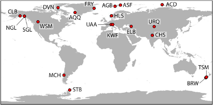
world glaciers and ice caps, and three synthetically generated of the real-world test cases is given in Figure 1.
glacier geometries (Table 1). Eighteen of the 20 real-world cases For every test case, glacier outlines, a digital elevation model
and all of the synthetic cases were identical to the ones used (DEM) of the glacier surface, and a set of ice thickness
within ITMIX1, whilst two additional test cases (Austre observations were available. These data were retrieved from a
FIGURE 1 | Overview of the real-world test cases considered in the frame of ITMIX2. Abbreviation keys as well as basic information for each glacier and data
avialability are given in Table 1.
Frontiers in Earth Science | www.frontiersin.org 3 January 2021 | Volume 8 | Article 571923Farinotti et al. Results of ITMIX2
variety of sources (see Supplementary Table S1). For 15 of the Experiment 03 (“flat-part bias”) is a configuration in which the
real-world cases, additional data were available for characterizing available profiles are preferentially located in the flat parts of the
the glaciers. Depending on the case, these included information of glacier. Logistics and accessibility make such a situation common
the surface mass balance, rate of ice thickness change, or surface for ground-based ice thickness surveys. The experiment was
ice flow speed and direction. Where available, the information constructed by using the available DEMs to determine the
was provided as a gridded product, with a horizontal resolution local surface slope at every measurement point of a given
ranging between 5 m (e.g., Washmawapta Glacier) and 1 km profile, calculating an average slope per profile, ranking the
(Devon Ice Cap) depending on the test case. An overview of profiles with respect to this average slope, and selecting the
the main characteristics and of the information available for each quarter of profiles with the lowest slopes. As for experiment
test case is given in Table 1. 02, the longitudinal profile was excluded.
Of particular relevance for ITMIX2 were the available ice Experiment 04 (“longitudinal profile only”) only provided the
thickness observations. As is virtually always the case when longitudinal profile for calibration. This configuration is
acquiring such observations in the field, these data were sometimes encountered for airborne surveys of valley glaciers
aligned along a series of individual transects. For ITMIX2, (e.g., Conway et al., 2009; Gourlet et al., 2016), when aircraft
these transects were segmented into individual profiles and manoeuvrability prevents across-flow profiles to be acquired.
numbered, giving rise to between 3 (Tasman Glacier) and 55 Experiments 05–08 (“80% of profiles retained”) are four
(South Glacier) individual profiles per test case. To ensure different layouts in which 80% of the available profiles are
compatibility with the provided gridded products, and to retained for calibration. The four realizations are generated by
avoid over-weighting of very densely sampled profiles in randomly selecting a corresponding number of profiles. Similarly,
particular, the data along these profiles were spatially re- Experiments 09–12 (“50% of profiles retained”) and 13–16 (“20%
sampled. This was done by moving along the defined profiles of profiles retained”) are, each, four random realizations of
at incremental steps of one cell size (e.g., 5 m in the case of layouts including 50% and 20% of the available profiles,
Washmawapta Glacier, or 1 km in the case of Devon Ice Cap), respectively.
and averaging any ice thickness observation within a radius of
half the cell size. The averaging was performed for both the 2.3 Call for Participation and Provided
observed thickness and the observed coordinates. This procedure Instructions
resulted in a thinning of the available observation, with between An open call for participation to ITMIX2 was posted on “cryolist”
30 (Tasman Glacier) and 5,411 (Austfonna Ice Cap) point (http://cryolist.org/) on May 07, 2018. Modellers that had
observations per test case (see Table 1). The thinned profiles participated in ITMIX1 (see Section 4 in Farinotti et al., 2017)
were at the basis of the IMTIX2 experiments described hereafter. were additionally contacted on a bilateral basis and encouraged to
participate. ITMIX2 instructions were provided on a dedicated
2.2 Experimental Design web-page and data access was granted upon email-registration.
For every ITMIX2 test case, 16 experiments were defined. In each Participants were asked to use the provided data to produce an
of these experiments, the available profiles were split into two estimate of the ice thickness distribution for as many test cases as
different subsets; one was made available for model calibration possible and for each of the 16 experiments. Any approach
(“calibration profiles”), and the other was used for validation of capable of estimating glacier ice thickness from the provided
the results (“test profiles”). The 16 experiments aimed at input data was admitted to participation, independently of
investigating both the effect of some peculiar layouts for the whether the approach was previously published in the
spatial distribution of the calibration profiles (experiments literature or not.
01–04), as well as the effect of the amount of data available Registered participants were provided access to all available
for calibration (experiments 05–16). Figure 2 visualizes the data at once, notably including all available ice thickness
different layouts for the example of Freya Glacier. measurements as well. The requirement of only using a given
Experiment 01 (“low-elevation bias”) mimics the situation in subset of the measurements for model calibration during the
which the available profiles are clustered toward the glacier’s individual experiments was, thus, not controlled further but relied
lowermost elevations. Such a configuration is sometimes on the honesty of each participant.
encountered for ground-based ice thickness surveys (e.g., Hagg To gauge the participants’ efforts and to ensure that a given
et al., 2013; Feiger et al., 2018) when the access to higher elevations subset of test cases would be considered by all participants, a
is hampered by logistics or safety constraints. For any glacier, the priority was assigned to every test case (cf. Table 1). Three cases
experiment was produced by selecting those profiles that are (Austfonna, Unteraar, Synthetic1) were defined as “compulsory”
located in the lowest quarter of the glacier’s elevation range. (priority “1”), meaning that a given approach had to provide
Experiment 02 (“thickest-parts bias”) represents the situation results for at least these three cases for being considered within
in which the available profiles preferentially capture the thickest ITMIX2. The other test cases were assigned priorities “2” (high
parts of the glacier. To do so, all profiles were ranked according to priority), “3” (to be considered if possible), or “4” (low priority).
the maximal ice thickness measured within each profile, and the The three test cases with priority “1” include a mountain glacier,
first quarter of the profiles was chosen. The longitudinal profile an ice cap, and a synthetic glacier. “Priority 4” was assigned to test
was excluded to avoid producing results similar to experiment 04 cases with comparatively sparse data availability. Priorities “2”
(see below).
Frontiers in Earth Science | www.frontiersin.org 4 January 2021 | Volume 8 | Article 571923Farinotti et al. Results of ITMIX2 FIGURE 2 | Profile layout for the 16 experiments considered within ITMIX2. Profiles indicate locations for which measured ice thickness is available. For each experiment (exp01 to exp16), a given subset of profiles was available for model calibration (red) whilst the remaining subset was used for validation (gray). Experiments 01–04 refer to peculiar configurations (see note within each panel) whilst experiments 05–16 consist of random selections of a given subset of profiles. The example refers to Freya Glacier, which is the non-compulsory test case considered by the largest number of modellers (cf. Table 2). Note the scalebar in the bottom right panel. and “3” roughly follow data availability (higher priority for better considered to be completed if results for all 16 experiments were data coverage) and aimed at having a mixture of test-case types submitted. (mountain glaciers, ice caps, synthetic cases). A test case was Frontiers in Earth Science | www.frontiersin.org 5 January 2021 | Volume 8 | Article 571923
Farinotti et al.                                                                                                                    Results of ITMIX2

3 PARTICIPATING MODELS AND                                                  additional term in the cost function that penalizes the misfit
SUBMITTED RESULTS                                                           between modeled and observed bedrock elevation. Thus, the
                                                                            procedure iteratively adjusts bedrock elevation, effective mass
A total of 13 models participated in the experiment, providing an           balance, ice hardness, and basal traction such that both mass and
ensemble of 2,544 individual solutions (159 test cases with 16              momentum are conserved while adjusting free parameters to
experiments each) in total (Table 2). The individual models are             most closely match observations of bedrock elevation, surface
briefly described hereafter, whilst an overview of the submitted             elevation, and surface velocity. This minimization is performed
results is given in Section 3.2. Within the set of models, three            using a simple gradient-descent procedure, with gradients
clusters can be discerned—the clusters being defined by the                  computed through the adjoint method.
similarity between individual approaches and their origin.
Providing a quantitative metric for the degree of similarity                3.1.2 Farinotti
between approaches would be difficult but Figure 3 visualizes                Sometimes referred to as Ice Thickness Estimation Method
the genealogy of the individual models. In principle, most models           (ITEM), this model is fully described in Farinotti et al.
descend from the approaches presented by (1) Linsbauer et al.               (2009b). In it, the considered glacier is subdivided into
(2009), which applies the shallow ice approximation and an                  individual ice-flow catchments, and an estimate of the ice
empirical relation between glacier elevation range and basal                volume flux across transects aligned along manually-defined
shear stress (Haeberli and Hoelzle, 1995) at the local scale, (2)           flow lines is solved for ice thickness by using a rearranged
Farinotti et al. (2009b), which is a flowline-based approach                 form of Glen’s flow law (Glen, 1955). The ice volume flux is
considering mass conservation and Glen’s ice flow law (Glen,                 obtained by integrating the glacier’s surface mass balance
1955), or (3) Morlighem et al. (2011), which is based on a two-             distribution, which itself is derived from the glacier’s the
dimensional consideration of the continuity equation. The                   surface topography.
ensemble-approach GilletChaulet is of different nature, as it                  For calibration, the procedure described in Farinotti et al.
uses the composite result that emerged from ITMIX1 as a                     (2009a) was used. In a nutshell, the correction factor C (see Eq. 7
prior for estimating the ice thickness at locations far away                in Farinotti et al., 2009b) was adjusted to minimize the misfit
from measurements (see Section 3.1.5 for details). To provide               between observed and modeled ice thickness at every profile with
context to the performance of individual models, a trivial estimate         observations. The factor C accounts for a number of assumptions,
based on the average thickness of the thickness measurements                including i) the linear shear stress distribution, ii) the
available during calibration is considered as well (Section 3.1.14).        approximation of the ice volume flux at the center of the
                                                                            profile with the average volume flux, and iii) the linear
3.1 Description of Individual Models and                                    relation between basal sliding and surface flow speed. In any
Calibration Strategy                                                        ITMIX2 experiment, C was adjusted independently for every
Nine of the 13 models participating to ITMIX2 already                       profile available for calibration. Between profiles, the values were
participated in ITMIX1, whilst four (the ensemble-approach                  linearly interpolated, whilst the average value was used at the start
GilletChaulet, and the models Maurer, TamreBraun, and                       and end of each flow line. Since C was adjusted on a profile-by-
Werder) joined anew. Hereafter, the models are briefly                       profile basis, deviations between measured and observed point
described in alphabetical order, with an emphasis on the                    thicknesses still occurred. These deviations were bi-linearly
calibration strategy chosen in the frame of ITMIX2. For                     interpolated in space, and the so-obtained field of differences
further details, the reader is referred to the original publications.       was subtracted from the estimated ice thickness distribution. This
                                                                            ensured a close match between modeled an observed thickness at
3.1.1 Brinkerhoff                                                           every observational point.
This model was labeled Brinkerhoff-v2 in ITMIX1 and is a further
development of the approach described in Brinkerhoff et al.                 3.1.3 Fuerst
(2016). In brief, the approach consists of a forward model                  This model was presented in Fürst et al. (2017), and consists of a
based on the Blatter-Pattyn approximation to the Stokes                     two-step inverse approach solving for mass conservation. In the
equations (Pattyn, 2003), and minimizes a cost-function                     first step, a geometrically controlled, non-local flux solution is
including three terms penalizing i) differences between                     converted into ice thickness by relying on the shallow ice
modeled and observed surface elevations, ii) strong spatial                 approximation (Hutter, 1983). When available, observations of
variations in bedrock elevations, and iii) non-zero ice                     ice flow velocities are then used in a second step to adjust the ice
thickness outside the glacier margin with respect to bedrock                thickness distribution. To solve for mass conservation, the model
elevation and effective surface mass balance. As an optional                uses Elmer/Ice, an open source finite element software (Gillet-
additional step, a spatially-varying basal traction and/or ice              Chaulet et al., 2012; Gagliardini et al., 2013).
hardness field is adjusted such that the misfit between                           For the individual ITMIX2 experiments, the model’s standard
modeled and observed velocity is minimized. Further details                 iterative inversion procedure was used. In the first step, ice
are found in Supplementary Section S1.2 of Farinotti et al. (2017).         velocities were ignored and the flux solution was directly
   For the different ITMIX2 experiments, calibration was                    translated into thickness values via the shallow ice
performed as for ITMIX1, but with the addition of an                        approximation. In this case, the unconstrained viscosity

Frontiers in Earth Science | www.frontiersin.org                        6                                    January 2021 | Volume 8 | Article 571923
Frontiers in Earth Science | www.frontiersin.org
Farinotti et al.
TABLE 2 | Overview of the submitted model results.
Glacier h Brinkerhoff Farinotti Fuerst Gantayat GilletChaulet Huss Maurer Morlighem Rabatel Ramsankaran TamreBraun VanPeltLeclercq Werder Total
(m)
ASF Austfonna 372.9 x x x x x x x x x x x x x 13
UAA Unteraar 142.5 x x x x x x x x x x x x x 13
SY1 Synthetic 1 96.3 x x x x x x x x x x x x x 13
SY2 Synthetic 2 125.3 x x x − x x x x − − x x x 10
SY3 Synthetic 3 126.4 x x x − x x x − − − x x x 9
FRY Freya 93.2 x x x − x x x − − x − − x 8
KWF Kesselwandferner 82.3 x x x − − x x − − x − x x 8
BRW Brewster 74.5 x x x − − x x − − − − x x 7
HLS Hellstugubreen 75.5 x x x − − x x − − − − x x 7
SGL South Glacier 60.9 x x x − x x x − − − − − x 7
ACD Academy of Sciences 395.0 − x − − x x x − − − − x x 6
− − − − − − −
7
MCH Mocho 79.6 x x x x x x 6
TSM Tasman 163.1 − x − x − x x − − x − − x 6
URQ Urumqi Glacier No. 1 45.2 x x x − x x − − − − − − x 6
AGB Austre Grønfjordbreen 86.2 x x x − − x x − − − − − − 5
CHS Chhota Shigri 102.7 − x − − − x x − − x − − x 5
ELB Elbrus 52.1 x x x − − x x − − − − − − 5
STB Starbuck 328.4 − x − − x x x − − − − − x 5
AQQ Aqqutikitsoq 59.4 − x − − − x x − − − − − x 4
CLB Columbia 195.2 − x − − − x x − − − − − x 4
DVN Devon 329.8 − x − − − x x − − − − − x 4
NGL North Glacier 78.0 − x − − − x x − − − − − x 4
WSM Washmawapta 72.7 − x − − − x x − − − − − x 4
Total 13 23 14 4 10 23 22 4 3 7 5 10 21 159
Glaciers are sorted according to the number of models by which they were considered. For any glacier, “x” indicates that all 16 experiments were performed by the corresponding model (columns). h is the mean ice thickness as obtained by
January 2021 | Volume 8 | Article 571923
averaging all model results submitted for a given glacier.
Results of ITMIX2Farinotti et al. Results of ITMIX2
FIGURE 3 | Overview of the models participating to ITMIX and their genealogy. Models are organized by their main setup (given to the left) and descendances are
indicated by solid lines. The setup distinguishes between i) local, point-based methods, ii) methods that are based on ice flowlines, elevation bands, or cross-sections,
and iii) methods based on two-dimensional considerations. The method GilletChaulet is a special case, as it is based on an ensemble of methods that have any of the
three setups. The color of each box indicates whether a given model participated in ITMIX1, ITMIX2, or both (see legend). The “velocity flag” indicates whether an
approach strictly requires ice flow velocities (asterisk) or whether it is able to use them when available (asterisk in brackets).
parameter was directly calibrated to reproduce each point Model calibration for individual ITMIX2 experiments was
measurement of ice thickness. After inserting the average performed by determining a specific shape factor f (see Eq. 2 in
viscosity as inferred from all available measurements, the Gantayat et al., 2014) at the points of intersection between
sparse viscosity information was linearly interpolated over the branchlines and profiles with ice thickness observations. For
drainage basin. If 2D information on ice velocity was available, any of these points (step 1), the value of f was chosen as to
the inversion directly solved for the ice thickness field. In this minimize the difference between modeled and observed ice
second step, the resulting thickness mismatch was an additional thickness. For branchline-points in the vicinity of available
term in the cost function that is iteratively minimized. profiles (step 2), the average f-value of these profiles was
assigned. For branchline-points farther apart, f was taken as
3.1.4 Gantayat the average of all values determined in the previous two steps.
This model, described in Gantayat et al. (2014), relies on the
equation of laminar flow (Cuffey and Paterson, 2010) and 3.1.5 GilletChaulet (Ensemble-Approach)
requires distributed information of the ice flow velocity at the This approach differs from the other models as it relies on the
glacier surface. A constant relation is assumed between surface ice results that were submitted to ITMIX1. In a nutshell, an optimal
flow velocity and basal sliding, whilst the basal shear stress is interpolation scheme is used to combine the multi-model
computed on the basis of surface slope (Haeberli and Hoelzle, ensemble from ITMIX1 with the observations available for
1995). For ITMIX2, discrete points along manually digitized calibration. Close to the observations, the measured ice
branchlines were considered, and the resulting ice thickness thickness is returned; in the far field (i.e., ca. 10 times the
was spatially interpolated by using the ANUDEM algorithm maximal thickness away), the approach returns the ensemble-
Hutchinson (1989) and assuming zero ice thickness at the mean thickness of ITMIX1.
glacier margin. The branchlines were generated requiring i) a More specifically, the approach is based on the Best Linear
lateral spacing of ca. 200 m between adjacent lines, ii) a minimal Unbiased Estimator (BLUE) (e.g., Goldberger, 1962). Assuming a
distance of 100 m from the glacier margin, and (iii branchlines linear relation between a prior estimate hb (referred to as to the
from individual glacier tributaries gradually merging into the background) and the observations ho , the BLUE estimator ha is
main tributary. the one that minimises the error variances, and is given by
Frontiers in Earth Science | www.frontiersin.org 8 January 2021 | Volume 8 | Article 571923Farinotti et al. Results of ITMIX2
ha hb + K ho − H hb (1) thickness distribution after smoothing. Finally, the thickness
distribution was spatially interpolated based on the available
where H is the observation operator, and K is a function of the thickness observations, the adjusted model results in
background error covariance matrix B and the observation error unmeasured regions, and the condition of zero thickness on
covariance matrix R: the glacier margin.
−1
K B HT H B HT + R . (2) 3.1.7 Maurer
The assumptions are that the background and the This model was presented as the Glacier Thickness Estimation
observations are unbiased, and that both have independent (GlaTE) framework in Langhammer et al. (2019a). It was
errors. HT is the matrix transpose of H. specifically designed for combining the modeling results with
The individual ITMIX2 experiments were addressed by taking measured ice thickness in an inversion procedure. This inversion
ho as the set of observations available for calibration. Observation follows the bed-stress approach by Clarke et al. (2013), which
errors were assumed to be uncorrelated and to have a standard subdivides a glacier into individual ice flow sheds and uses an
deviation of 5 m (note that no information was provided on the estimate of the glacier ice volume flux to invert for ice thickness
actual accuracy of these observations within ITMIX2). H was based on Glen’s flow law. The strength of the GlaTE framework is
chosen to be an operator that interpolates the ice thickness from the capability of both modularly adding further observational
the uniform grids used in ITMIX1 to the locations of the available constraints—such as observed ice flow velocities or rates of ice
thickness observations. For the background, the ITMIX1 average thickness change for example—and accounting for observational
composite solution (cf. Farinotti et al., 2017) was used, with the uncertainties when available. GlaTE is open-access software and
covariance matrix B being estimated from the ITMIX1 ensemble. it is available at https://gitlab.com/hmaurer/glate.
The ITMIX1 ensemble comprises between 4 (Starbuck) and 16 The calibration procedure used for ITMIX2 followed the
(Synthetic1) individual model members, with an average of 10 original approach (Langhammer et al., 2019a). In a nutshell,
members. Since covariance matrices estimated from small GlaTE sets up a system of equations comprising 1) constraints
ensembles can exhibit spurious long-range correlations, a that force observed and predicted ice thickness data to match
domain localization technique was used. This technique within a prescribed accuracy, 2) glaciological modeling
ensured that the thickness at a given location was updated constraints that force the ice thicknesses to comply with the
using only observations that are within 10 times the maximum model of Clarke et al. (2013), supplemented by longitudinal
ice thickness of the background field. For locations farther apart, averaging as proposed by Kamb and Echelmeyer (1986), 3)
the ITMIX1 composite solution remains unchanged. The boundary constraints that force the ice thickness to be zero
procedure was implemented by using the Localized Ensemble outside of the glacier outlines, and 4) smoothness constraints
Transform Kalman Filter (Hunt et al., 2007) as provided in the that force the ice thickness distribution to vary smoothly. The
Parallel Data Assimilation Framework by Nerger et al. (2005). For contributions of the individual constraints can be controlled by
further details and an application of the ensemble Kalman Filter weighting factors. Since the smoothness constraints are the least
in the context of ice flow modeling, see Gillet-Chaulet (2020). physical ones, GlaTE attempts to minimize the corresponding
weighting factor. More specifically, a relatively high factor is
3.1.6 Huss chosen at the start and then gradually decreased until the
Sometimes referred to as HF-model, the approach was originally observed and predicted thicknesses match within the
presented for a global-scale ice thickness reconstruction in Huss prescribed error bounds. For ITMIX2, the consistency of the
and Farinotti (2012). The model is based on the concepts of individual inversion runs was maximized by using the same
Farinotti et al. (2009b) but avoids the necessity of defining ice flow control parameters for all experiments. This also allowed the
lines and catchments by performing all computations for 10 m computations to be performed in an automated fashion.
elevation bands. Variations in the valley shape and basal shear
stress along the glacier’s longitudinal profile are taken into 3.1.8 Morlighem
account, as are the temperature-dependence of Glen’s flow This model was originally presented in Morlighem et al. (2011)
rate factor (Glen, 1955) and the variability in basal sliding. and is now also known as BedMachine (Morlighem et al., 2017;
Average elevation-band ice thickness is extrapolated on a Morlighem et al., 2020). It is specifically designed to provide
regular grid by considering both local surface slope and estimates of ice thickness between transects surveyed by radio-
distance from the glacier margin. echo soundings, and was developed for applications over ice
For ITMIX2, calibration of individual experiments was sheets, rather than mountain glaciers. The model is cast as an
performed by a three-step procedure including (i model optimization problem minimizing the misfit between observed
optimization, (ii longitudinal bias correction, and (iii spatial and modeled thicknesses. Being based on mass conservation, the
interpolation. First, the apparent mass balance gradient (Huss ice thickness is computed by requiring the ice flux divergence to
and Farinotti, 2012) was calibrated to minimize the average misfit be balanced by the rate of thickness change and the net mass
with the available ice thickness observations. Second, the relative balances. When surface ice velocities were not provided, the
deviation of the modeled thickness was evaluated in 50 m shallow ice approximation was applied by assuming that
elevation bands, and superimposed over the computed ice internal deformation was about half of the total surface speed.
Frontiers in Earth Science | www.frontiersin.org 9 January 2021 | Volume 8 | Article 571923Farinotti et al. Results of ITMIX2
The ice thickness was then determined by solving the resulting 3.1.11 TamreBraun
polynomial. This model has not been published so far. It is based on mass
The ITMIX2 experiments were addressed by using the model’s conservation, requiring ice flux divergence to be matched by mass
standard framework (Morlighem et al., 2011) and did not require balance and rate of ice thickness change. Ice thickness at any
any specific amendment. point on the glacier is directly computed by integration of mass
balance over its catchment area. The latter is determined by
3.1.9 Rabatel repurposing the FastScape algorithm (Braun and Willett, 2013)
This model was first presented in the frame of ITMIX1, and is from its use in geomorphology. Ice flow parameters in the model
now fully described in Rabatel et al. (2018). In brief, the ice are optimized for the smallest misfit between modeled and
volume flux across individual cross-sections is quantified from observed ice thicknesses where such observations are available.
information of the glacier’s surface mass balance and observed A more comprehensive description of the model is found in
surface flow velocities. Using Glen’s flow law, this information is Supplementary Section S1.
translated in an average ice thickness for each cross-section. This For ITMIX 2, the model parameters fd (i.e., the pre-factor for
thickness is then first distributed along each cross-section by the deformation velocity) and fs (i.e., the pre-factor for the sliding
assuming a constant relation between local thickness and surface velocity) were optimized to minimize the misfit (hmod − hobs )2 .
velocity, and then interpolated between cross-section by using Here, hmod and hobs are the modeled and observed ice thickness at
universal Kriging with anisotropy in the main glacier flow a give location, respectively. The sum was computed over all
direction. Note that the model requires information about thickness data points available in a given experiment, and the
surface ice flow speeds, thus reducing the set of test cases that results of the run with the lowest misfit were submitted. The
can considered. parameter space was explored using the neighborhood algorithm
Model calibration for individual ITMIX2 experiments (Sambridge, 1999a; Sambridge, 1999b). Note that the algorithm is
followed the procedure described in Rabatel et al. (2018). For versatile enough to deal with larger parameter spaces—such as
each experiment, the ratio between local ice thickness h and local when mass balance data is not available and needs to be inferred
surface ice flow speed v is quantified for every grid cell. This ratio as well—although such cases were not considered.
is then plotted against the surface elevation z, and a regression of
the form h/v f (z) is performed. The type of regression (linear 3.1.12 VanPeltLeclercq
or polynomial) is chosen using the profiles available for This model is an adaptation of the approach by van Pelt et al.
calibration in order to minimize the difference between (2013), as described in Supplementary Section S1.17 of Farinotti
observed and modeled thickness when computing h v · f (z). et al. (2017). Following the concepts laid out in Leclercq et al.
This inverse relation is then applied to the entire glacier by (2012), the model derives an ice thickness distribution by
making use of the distributed information of both z (from the iteratively minimizing the misfit between modeled and
DEM) and v (from the maps of ice flow speed). Note that the form observed elevations of the glacier surface. SIADYN—an ice
of the relation between h and v could be extended to include dynamics model relying on the vertically integrated shallow ice
additional morphologic variables (such as surface slope or approximation—is used as a forward model (SIADYN is part of
distance to the glacier margin, for example) or to be non- the ICEDYN package; for more details, see Section 3.3 in Reerink
linear (Bolibar et al., 2020). et al., 2010) whilst basal sliding is included through a Weertman-
type formulation (Huybrechts, 1991). In absence of time-
3.1.10 Ramsankaran dependent mass balance information, every forward model run
This model was labeled RAAJglabtop2 in ITMIX1, is known as uses a fixed surface forcing, and continues until a steady state is
GlabTop2_IITB version (Ramsankaran et al., 2018; Pandit and reached.
Ramsankaran, 2020), and is an independent re-implementation For the ITMIX2 experiments, an extensive 2D parameter
of the approach described in Frey et al. (2014). The approach itself exploration was performed. In particular, the model was set
is based on the concepts presented in Linsbauer et al. (2012) with up for every test case with a varying number of iterations
the difference of being entirely grid-based. The local ice thickness (that is the number of iterative steps in which the subglacial
is first calculated for a set of randomly selected grid cells, which is topography is adjusted) and a range of flow enhancement factors.
done from an estimate of both the basal shear stress and the All combinations were run, and the combination that minimized
surface slope. This thickness is then spatially interpolated by the root mean square error between observed and modeled ice
assigning a minimum, non-zero thickness to grid cells directly thicknesses was selected. Typically, a few hundred combinations
adjacent to the glacier margin. were tested before selecting the optimal ones. Within ITMIX2, 16
For the individual ITMIX2 experiments, the model was different combinations were chosen for every test case, depending
calibrated by varying the dimensionless shape factor f (see on the configuration of the ice thickness data available for
Eq. 1 in Ramsankaran et al., 2018) over four levels, calibration within each experiment.
i.e., f 0.6, 0.7, 0.8, and 0.9. By doing so, f was assumed to
be identical for all profiles, and the value resulting in the lowest 3.1.13 Werder
root mean square error between modeled and observed ice This approach was presented as the Bayesian Ice Thickness
thickness was chosen. Estimation (BITE) model in Werder et al. (2020), where it is
Frontiers in Earth Science | www.frontiersin.org 10 January 2021 | Volume 8 | Article 571923Farinotti et al. Results of ITMIX2
described in full detail. In brief, the approach consists of a forward cases. In some instances, the time required for model set up was a
model based on the approach by Huss (cf. Section 3.1.6) deterrent for considering more cases (note that both ITMIX1 and
augmented with the capability of calculating surface flow ITMIX2 were community efforts run without funding and purely
speeds consistent with mass conservation. The mass based on voluntary commitment). In the end, every test case was
conservation and shallow ice calculations are first conduced on considered by at least four different models, and ten test cases
elevation bands, with the resulting ice thicknesses and flow speeds were considered by more than half of the models.
being then extrapolated to the map plane. The model is fitted to
ice thickness and flow speed observations (when available) using
a Bayesian approach. When observational uncertainties are 4 EVALUATION PROCEDURE
known, the Bayesian formulation allows for this information
to be taken into account. 4.1 Consistency Checks and Adjustments
The individual ITMIX2 experiments were addressed by using Prior to further evaluation, the submitted results were checked for
a calibration procedure similar to the one described in Werder consistency and adjusted if necessary. First, any non-zero ice
et al. (2020): for each experiment, the model is fitted to the thickness outside of the provided glacier margins was discarded,
available profiles with ice thickness observations and to the meaning that all further evaluations refer to the area within that
distributed surface flow speeds; unlike in the original margins; negative or missing thicknesses within the margin
procedure, however, the glacier length is not used for fitting. (which affect roughly 1% of all submitted grid cells and arise
The error between observations and model predictions—used in for some models when the velocity input fields have data gaps)
the likelihood calculation—are assumed to be normally were set to a no-data value and were discarded from further
distributed with a standard deviation of 15 m for ice thickness analysis. Second, the extent and resolution of the results were
and 30 m a−1 for flow speed. Fitted model parameters include the adjusted as to match the originally-provided gridded data (cf.
apparent mass balance, the sliding factor, the ice temperature, and Section 2.1). Trimming of the spatial extent was necessary for
two parameters affecting the extrapolation from elevation bands some submissions of Gantayat and Fuerst, whilst a re-sampling of
to the map plane. The prior distributions of the parameters are the resolution from 50 m grid spacing to 300 m spacing was
determined by the available data or, if unavailable, by expert necessary for GilletChaulet’s Austfonna results. The trimming of
guesses. The fitting procedure is implemented with a Markov the extents did not require any interaction with the provided ice
chain Monte Carlo method with 105 steps. thickness estimates (since only the far, non-glacierized margins
were affected), whilst the re-sampling in the case of Austfonna
3.1.14 The Simplest Model as a Benchmark was performed by computing averages of the 36 cells with 50 m
To provide context to the performance of the above models, an resolution contained within each 300-m cell. The cause of these
additional, trivial estimate of the ice thickness distribution was discrepancies can be traced back to the affected models using the
computed. For any test case and experiment, this estimate simply topography-data distributed within ITMIX1, rather than
consisted of the average ice thickness of the profiles available for ITMIX2. We stress that both the trimming and the re-
calibration. The estimate is assumed to be valid at any location sampling do not alter the ice thickness estimates, and note
(homogeneous thickness). We refer to this simplest possible that the no-data values introduced through the first
estimate as to the benchmark, indicating that any model with adjustment step only potentially affect the results when they
a performance lower than this can be considered as virtually skill- concern grid-cells that are intersected by measurement profiles
free. (i.e.,Farinotti et al. Results of ITMIX2
field campaign, and systematic interpretation errors are thus median σ n of 17.2%. Low values, instead, are found for
difficult to exclude. Brinkerhoff, Gantayat, the ensemble-approach GilletChaulet,
To enable direct comparison between modeled thicknesses Rabatel, VanPeltLeclerq and Werder, which all have σ n
(which are gridded) and observed thicknesses (which refer to medians below 13%. A remarkable exception is the model
multiple profiles and can be available at any location), the Ramsankaran, for which the median σ n is close to zero. This
observed thicknesses are first rasterized on the modeling grid. means that the model provides the same solution independently
For every grid-cell, this is done by computing the arithmetic of the profiles used for model calibration, and indicates that the
average of all observations that fall within that cell. To allow for chosen calibration procedure (cf. Section 3.1.9) tended to select
comparability between test cases of different size and thickness, the same shape factor for all experiments. We note that this could
deviations are further expressed as percent-deviations from the be resolved by following a calibration procedure such as the one
mean ice thickness of the corresponding test case. Since the “true” adopted in Ramsankaran et al. (2018), who defined a variable
mean ice thickness is unknown, it is computed by averaging all shape factor depending on elevation and other topographical
model results submitted for a given test case; that is, the average properties.
thickness is the result of averaging over all models, all The above model behavior is confirmed by the indicator Δhc ,
experiments, and all grid-cells of that particular case (the i.e., by the deviation of the modeled ice thickness at the
resulting values are given in Table 2). This evaluation strategy calibration profiles (again, the quantity is first computed
follows the one used during ITMIX1, and ensures that average individually for every location and model, and then pooled
percent-deviations are not skewed by large relative deviations that across test cases and experiments). Whilst most models show
may occur when local thickness is small. For a hypothetical a distribution of Δhc centered around zero (Figure 4C),
glacier that is 50 m thick on average, for example, Ramsankaran shows median deviations in the order of +50%,
overestimating the thickness of a 1 m-thick marginal grid-cell thus indicating a systematic overestimation of the actual
by say, 10 m, results in a deviation of +20%, and not +1, 000% as if thickness. Slight biases are also found for Gantayat and
point-thickness were considered. TamreBraun, with median Δhc in the order of −15%. The
distribution of Δhc also reveals that some models aim at
matching the calibration data exactly (e.g., Farinotti, Fuerst,
5 RESULTS AND DISCUSSION the ensemble-approach GilletChaulet and Maurer have
interquartile ranges below 10%) whilst other approaches allow
5.1 Characteristics of Results Submitted by the modeled thickness to fluctuate around the measured thickness
Individual Models (the interquartile range for Brinkerhoff, TamreBraun and
The results submitted by individual models can be characterized VanPeltLeclerq, for example, is in the order of 30–40%). The
by three indicators: 1) the standard deviation σ n between latter is the expression of a compromise between agreement with
individual solutions at profiles that were not used for observations—which can be affected by unknown uncertainties
calibration (“test profiles”), 2) the deviation Δhn between and biases—and internal model consistency—which is governed
modeled and observed ice thickness at the test profiles, and 3) by the conservation of mass and/or momentum in the mentioned
the deviation Δhc between modeled and observed ice thickness for models. Again for comparison, the benchmark model shows an
profiles that were available for calibration. interquartile range of 60% whilst it is unbiased (Δhc ≈ 0%) by
The first indicator, σ n, quantifies the degree to which similar design.
solutions are produced when different calibration data are The indicator Δhn , finally, quantifies the models’ capabilities of
provided. High values suggest that a given model is very correctly predicting the ice thickness at unmeasured locations.
sensitive to these data, with very different results being The distribution of Δhn is shown in Figure 4B, and reveals that
provided depending on which subset of profiles was used for whilst the median deviations remain virtually unaltered and
calibration. Extremely low values, instead, indicate that the centered around zero in most cases, the difference between
calibration procedure is insensitive to the input. Moderate modeled and observed thickness increases significantly when
values might thus be preferential as they hint at a compromise compared to locations with thickness observations (cf.
between model robustness and sensitivity. To compute σ n for a indicator Δhc ). The first observation can be interpreted as a
given location, we determine the difference between modeled hm confirmation that the implemented calibration procedures are
and observed ho ice thickness for all experiments during which unbiased (pooled across models but excluding the results by
that point was part of the test profiles (that is a set of up to 16 Ramsankaran, the median deviation is −2.3% and −1.3% of
values), divide by the mean ice thickness h of the considered the mean ice thickness for the compulsory and all cases,
glacier, and compute the standard deviation of the so-obtained respectively). The second observation is expected, and is
differences (that is one value per location): expressed in a change of the interquartile ranges and
σ n stdev((hm − ho )/h). Figure 4A shows the distribution of confidence intervals, for example. On average over the 13
σ n when the quantity is pooled across all test cases and is stratified considered models, the two quantities increase by 10% and
by model. Large values of σ n are found for the models Morlighem 30% of the mean ice thickness, respectively. Of particular
and Farinotti, which show median σ n values of ∼ 30% the mean notice are the models that displayed a bias in Δhc . In those
ice thickness. For comparison, the benchmark model shows a cases, the distribution of Δhn is skewed. Such skewness is
particularly prominent in the model Ramsankaran (biased
Frontiers in Earth Science | www.frontiersin.org 12 January 2021 | Volume 8 | Article 571923You can also read