Identifying the sources of uncertainty in climate model simulations of solar radiation modification with the G6sulfur and G6solar Geoengineering ...
←
→
Page content transcription
If your browser does not render page correctly, please read the page content below
Atmos. Chem. Phys., 21, 10039–10063, 2021
https://doi.org/10.5194/acp-21-10039-2021
© Author(s) 2021. This work is distributed under
the Creative Commons Attribution 4.0 License.

Identifying the sources of uncertainty in climate model simulations
of solar radiation modification with the G6sulfur and G6solar
Geoengineering Model Intercomparison Project
(GeoMIP) simulations
Daniele Visioni1 , Douglas G. MacMartin1 , Ben Kravitz2,3 , Olivier Boucher4 , Andy Jones5 , Thibaut Lurton4 ,
Michou Martine6 , Michael J. Mills7 , Pierre Nabat6 , Ulrike Niemeier8 , Roland Séférian6 , and Simone Tilmes7
1 Sibley  School for Mechanical and Aerospace Engineering, Cornell University, Ithaca, NY, USA
2 Department    of Earth and Atmospheric Science, Indiana University, Bloomington, IN, USA
3 Atmospheric Sciences and Global Change Division, Pacific Northwest National Laboratory, Richland, WA, USA
4 Institut Pierre-Simon Laplace, Sorbonne Université/CNRS, Paris, France
5 Met Office Hadley Centre, Exeter, EX1 3PB, UK
6 CNRM, Université de Toulouse, Météo-France, CNRS, Toulouse, France
7 Atmospheric Chemistry, Observations, and Modeling Laboratory, National Center for Atmospheric Research,

Boulder, CO, USA
8 Max Planck Institute for Meteorology, Hamburg, Germany

Correspondence: Daniele Visioni (dv224@cornell.edu)

Received: 15 February 2021 – Discussion started: 9 March 2021
Revised: 12 May 2021 – Accepted: 4 June 2021 – Published: 6 July 2021

Abstract. We present here results from the Geoengineer-          temperature target (1.91 ± 0.44 %). The analyzed models al-
ing Model Intercomparison Project (GeoMIP) simulations           ready show significant differences in the response to the
for the experiments G6sulfur and G6solar for six Earth sys-      increasing CO2 concentrations for global mean tempera-
tem models participating in the Climate Model Intercompar-       tures and global mean precipitation (2.05 K ± 0.42 K and
ison Project (CMIP) Phase 6. The aim of the experiments          2.28 ± 0.80 %, respectively, for SSP5-8.5 minus SSP2-4.5
is to reduce the warming that results from a high-tier emis-     averaged over 2081–2100). With aerosol injection, the dif-
sion scenario (Shared Socioeconomic Pathways SSP5-8.5) to        ferences in how the aerosols spread further change some of
that resulting from a medium-tier emission scenario (SSP2-       the underlying uncertainties, such as the global mean precip-
4.5). These simulations aim to analyze the response of cli-      itation response (−3.79 ± 0.76 % for G6sulfur compared to
mate models to a reduction in incoming surface radiation as      −2.07 ± 0.40 % for G6solar against SSP2-4.5 between 2081
a means to reduce global surface temperatures, and they do       and 2100). These differences in the behavior of the aerosols
so either by simulating a stratospheric sulfate aerosol layer    also result in a larger uncertainty in the regional surface tem-
or, in a more idealized way, through a uniform reduction         perature response among models in the case of the G6sulfur
in the solar constant in the model. We find that over the fi-    simulations, suggesting the need to devise various, more spe-
nal two decades of this century there are considerable inter-    cific experiments to single out and resolve particular sources
model spreads in the needed injection amounts of sulfate         of uncertainty. The spread in the modeled response suggests
(29 ± 9 Tg-SO2 /yr between 2081 and 2100), in the latitudi-      that a degree of caution is necessary when using these results
nal distribution of the aerosol cloud and in the stratospheric   for assessing specific impacts of geoengineering in various
temperature changes resulting from the added aerosol layer.      aspects of the Earth system. However, all models agree that
Even in the simpler G6solar experiment, there is a spread        compared to a scenario with unmitigated warming, strato-
in the needed solar dimming to achieve the same global

Published by Copernicus Publications on behalf of the European Geosciences Union.
10040                                   D. Visioni et al.: Identifying the sources of uncertainty in climate model simulations

spheric aerosol geoengineering has the potential to both glob-       CO2 but no geoengineering. Two new experiments have been
ally and locally reduce the increase in surface temperatures.        proposed as part of the GeoMIP Phase 6 (Kravitz et al.,
                                                                     2013b) where geoengineering is aimed at lowering global
                                                                     mean surface temperatures from those in a high-tier emission
                                                                     scenario (Shared Socioeconomic Pathway; SSP5-8.5; Mein-
1   Introduction                                                     shausen et al., 2020) to those in a medium-tier emission sce-
                                                                     nario (SSP2-4.5). G6sulfur aims to achieve this temperature
Solar radiation modification (SRM) is defined as the pro-            goal by increasing the simulated stratospheric aerosol optical
posed artificial altering of the radiative balance of the planet     depth (AOD). In models with an interactive sulfur cycle and
in order to temporarily counteract some of the imbalance             stratospheric aerosol microphysics this is done by simulating
produced by the increase in atmospheric greenhouse gases             the injection of SO2 between 10◦ N and 10◦ S between 18
(GHGs). This might be achieved in multiple ways, but the             and 20 km, whereas in other models this is done by impos-
most studied one, originally proposed by Budyko (1977) and           ing a sulfate distribution calculated offline. G6solar, on the
Crutzen (2006), would consist of the injection of SO2 into           other hand, decreases total incoming solar irradiance. While
the stratosphere in order to produce a layer of sulfate aerosols     the latter does not aim to reproduce the effects of an actual
capable of partially reflecting incoming solar radiation; this       sulfate aerosol intervention, comparisons of its results with
is usually defined as stratospheric aerosol intervention (SAI)       simulations of stratospheric aerosols in the same model may
or sulfate geoengineering. Simulating such a technique in            help understand the contributions to inter-model differences
climate models is the main way to understand the possible            in the response to aerosols (Niemeier et al., 2013; Visioni
impacts on the composition of the atmosphere and on the              et al., 2021). Both reductions of incoming solar radiation at
surface climate to determine its eventual feasibility, under-        the surface (directly, by turning down the Sun, or indirectly,
stand its possible impacts on ecosystems and populations             by having the aerosols reflect the solar radiation) are adjusted
(Zarnetske et al., 2021) and inform policymakers and stake-          at least every decade to ensure that the target temperature is
holders.                                                             being met.
   The Geoengineering Model Intercomparison Project                     There are multiple uncertainties that can be investigated
(GeoMIP) was proposed initially in Kravitz et al. (2011)             with a multi-model intercomparison when considering the
as a way to standardize SRM modeling experiments,                    climate models’ responses to an artificial, deliberate mod-
allowing for a more robust comparison between model                  ification of surface temperatures by means of stratospheric
responses and determination of sources of uncertainties              aerosols (Kravitz and MacMartin, 2020). In the stratosphere,
and areas for improvement. Whereas the term “geo-                    these include the conversion of injected SO2 into strato-
engineering”, “climate engineering” or, more recently,               spheric aerosol and the subsequent large-scale distribution
“climate intervention” (https://www.silverlining.ngo/us-             of the aerosols by stratospheric circulation (not dissimilar to
national-survey-terminology-for-approaches-for-directly-             multi-model analyses of simulations of explosive volcanic
influencing-climate, last access: 28 June 2021) are also             eruptions; Marshall et al., 2018; Clyne et al., 2021), the
usually used to consider methods of carbon dioxide removal           chemical response of key stratospheric components (ozone,
(CDR), in the original intention of GeoMIP (and this work)           methane) to the aerosol layer (Pitari et al., 2014; Visioni
it was only considered as a more colloquial term for SRM.            et al., 2017b), the magnitude of the produced local heating
   Two previous experiments in particular have been widely           (Niemeier et al., 2020) and the dynamical response. At the
analyzed and discussed: G1, where the solar constant is re-          surface, uncertainties include the magnitude of the result-
duced in order to offset the temperature increase produced by        ing global cooling per Tg-SO2 injected or per unit of opti-
a 4× increase in CO2 compared to pre-industrial concentra-           cal depth produced, the regional patterns of change in tem-
tions (Kravitz et al., 2013b; Tilmes et al., 2013; Glienke et al.,   perature (Kravitz et al., 2013a), precipitation (Kravitz et al.,
2015; Russotto and Ackerman, 2018b; Kravitz et al., 2021),           2013b; Tilmes et al., 2013) and extreme events (Aswathy
and G4, where a constant amount of SO2 is injected into the          et al., 2015; Ji et al., 2018) as well as other variables that
equatorial stratosphere under emissions from the Representa-         might affect ecosystems and populations (Zarnetske et al.,
tive Concentration Pathway 4.5 (RCP4.5) (Pitari et al., 2014;        2021), such as tropospheric ozone (Xia et al., 2017) or cloud
Kashimura et al., 2017; Visioni et al., 2017b; Plazzotta et al.,     changes (Russotto and Ackerman, 2018a).
2019. However, previously performed GeoMIP experiments                  In this work we analyze the response to the two proposed
were not intended to be “realistic” deployments of geoengi-          experiments in six global climate models, all part of the Cli-
neering, either because they were performed under idealized          mate Model Intercomparison Project, Phase 6 (CMIP6), in
conditions (such as 4×CO2 concentrations) or because they            order to explore some of the described uncertainties in these
considered a fixed, constant amount of injected SO2 with an          state-of-the-art models. After briefly describing the partici-
abrupt beginning and ending. Furthermore, in the case of the         pating models and the experimental setups in Sect. 3.1, we
G4 experiment, there was no scenario to compare in which             first confirm that all models successfully manage to lower
similar global mean temperatures were achieved with lower            globally averaged surface temperatures from those of the un-

Atmos. Chem. Phys., 21, 10039–10063, 2021                                            https://doi.org/10.5194/acp-21-10039-2021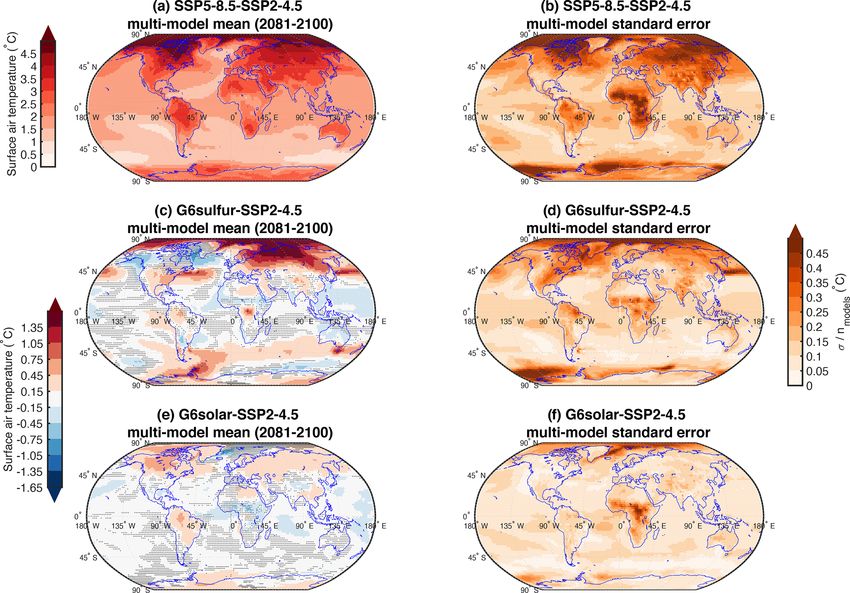
D. Visioni et al.: Identifying the sources of uncertainty in climate model simulations                                      10041

derlying high emission scenario to those of the medium one.         UKESM1-0-LL) injected SO2 uniformly between 10◦ N and
While in the case of a broad solar reduction there is no con-       10◦ S between 18 and 20 km of altitude and across a sin-
straint on the maximum achievable cooling, previous work            gle longitudinal band (◦ 0). CESM2(WACCM) injected SO2
has suggested a non-linear behavior between injected SO2            at the Equator and at 25 km of altitude. The others pre-
and aerosol burden at high amounts of injections (Pierce            scribed an already-calculated aerosol optical depth distri-
et al., 2010; Niemeier and Timmreck, 2015), resulting in a          bution: CNRM-ESM2-1 used an input dataset provided by
reduced efficiency. Therefore we also try to evaluate the pres-     GeoMIP (the aerosol distribution the G4SSA experiment;
ence of a similar non-linearity in the participating models (if     Tilmes et al., 2015), while MPI-ESM prescribed their own
it occurs in the range of forcing needed in our experiment).        aerosol distribution derived from the simulations described
We then analyze in Sect. 3.2 the differences in the latitudinal     in Niemeier and Schmidt (2017) and Niemeier et al. (2020).
spread of the stratospheric aerosols cloud despite the consis-      In both cases, the prescribed aerosols are fully integrated in
tent injection location. Even when pursuing the same global         the radiative transfer calculations. Therefore, the response
mean temperature-oriented goal, it has been shown in simu-          of direct and diffuse radiation at the surface and the local-
lations with CESM1(WACCM) that differences in the latitu-           ized stratospheric warming due to radiative heating are fully
dinal (Kravitz et al., 2019 and seasonal (Visioni et al., 2020b)    consistent with those from the other models where the full
distribution of the aerosols can result in significant differ-      aerosol production from SO2 is simulated (see, for instance,
ences in surface climate. If different models simulate differ-      Laakso et al., 2020). However, previous studies have shown
ent distributions of the aerosols (as for the G4 experiment;        the presence of non-linearities at higher injection loads.
Pitari et al., 2014) due to different stratospheric processes       These can be microphysical in nature, with aerosol particles
(both dynamical and chemical; Niemeier et al., 2020; Franke         growing to larger sizes with larger loads of SO2 (Niemeier
et al., 2021), the simulated surface climate would also be          and Timmreck, 2015), or dynamical, with the stratospheric
different. Furthermore, even given similar simulated aerosol        heating producing changes in stratospheric circulation result-
distribution, the stratospheric response might differ due to        ing in a different aerosol distribution in the tropics (Visioni
differences in aerosol optics and in the radiative transfer cal-    et al., 2018b) or at high latitudes (Visioni et al., 2020a). If
culation and in the representation of chemical processes in         the same aerosol distribution is simply scaled up, these effect
the stratosphere (i.e., if interactive chemistry is considered in   would not be present in those models.
the stratosphere; Franke et al., 2021) resulting in a different        A summary of the participating models, ensemble size and
dynamical and ultimately surface response (Simpson et al.,          notes related to the implementation of G6sulfur is provided
2019; Jiang et al., 2019; Banerjee et al., 2021), which we          in Table 1. Further information on the models’ components
discuss in Sect. 3.3 for annual mean temperature and precip-        can be found in the references provided for each model and
itation.                                                            a summary is given in Table S1 in the Supplement. More
                                                                    detailed information for CMIP6 models can also be found
                                                                    in Séférian et al. (2020) for marine biogeochemistry, Arora
2   Description of simulations                                      et al. (2020) for carbon-climate feedbacks and Thornhill et al.
                                                                    (2021) for atmospheric chemistry.
We analyze four sets of simulations from 2020 to 2100: two             Two modeling teams, IPSL-CM6A-LR and UKESM1-0-
baseline scenarios without geoengineering that follow two           LL, determined for every decade by how much to reduce
Shared Socioeconomic Pathways, SSP2-4.5 and SSP5-8.5                the solar constant or how much more SO2 or prescribed
(O’Neill et al., 2016), and two scenarios with geoengineer-         aerosols to have in the stratosphere in order to reduce surface
ing, G6solar and G6sulfur (Kravitz et al., 2015). Overall, six      temperatures of the forthcoming decade to SSP2-4.5 levels,
models participated in all experiments (Table 1).                   whereas four teams, CESM2(WACCM), MPI-ESM1.2-LR,
   In the SSP2-4.5 and SSP5-8.5, GHG emissions follow a             MPI-ESM1.2-HR and CNRM-ESM2-1, did so every year.
medium and high trajectory, respectively, resulting by the          For CESM2(WACCM), the determination of injected SO2
end of the century in a radiative forcing indicated by the          or reduction of the solar constant is done by a feedback al-
last two numbers in the name (i.e., 4.5 and 8.5 W/m2 , simi-        gorithm described in Kravitz et al. (2017) and also used in
lar to the Representative Concentration Pathways in CMIP5).         Tilmes et al. (2018a, 2020).
The G6 simulations start in 2020 with the same emissions as
SSP5-8.5 and, on top of that, have either the solar constant re-
duced by a certain fraction or produce a sulfate aerosol opti-      3     Results
cal depth with the aim of reducing the globally averaged sur-
face temperature down to the SSP2-4.5 level. While the solar        3.1    Magnitude of geoengineering required
reduction is performed in the same way in all G6solar exper-
iments, reducing the solar constant uniformly at all latitudes,     All models successfully reduce global mean surface air tem-
not all participating models included stratospheric aerosols        peratures to within 0.2 ◦ C of SSP2-4.5 levels on average
by directly injecting SO2 . Two models (IPSL-CM6A-LR and            throughout the century with both geoengineering methods

https://doi.org/10.5194/acp-21-10039-2021                                           Atmos. Chem. Phys., 21, 10039–10063, 2021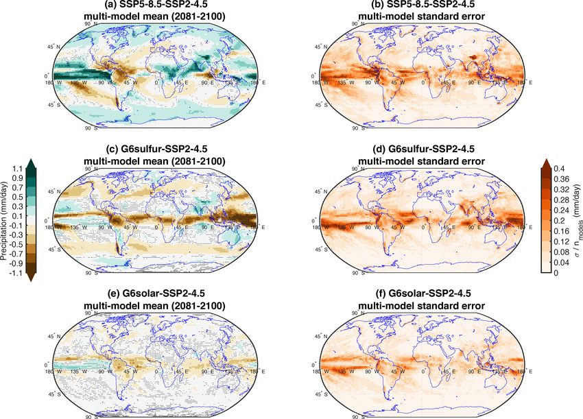
D. Visioni et al.: Identifying the sources of uncertainty in climate model simulations

                                                                                                                                                                                                                                                                                                    https://doi.org/10.5194/acp-21-10039-2021
                                                                                         Table 1. Summary of model simulations used in this work. The first column has the name of the model used, the DOI for the relative CMIP6 dataset as recommended by CMIP6 (see
                                                                                         Stockhause and Lautenschlager, 2021) and the horizontal and vertical resolution; the second column indicates the main scientific reference(s) where the model version is described.
                                                                                         Columns 3 to 6 show the size of the ensemble analyzed in this work. For some models, more ensemble members are available for the SSP experiments, but only those with the same
                                                                                         variant as the G6 experiments are used in this work. Finally, the last two columns indicate the source of stratospheric aerosols for G6 and the presence of interactive stratospheric ozone.
                                                                                         All models have interactive marine biogeochemistry and are coupled to an interactive land model.
                                                                                           Model name and CMIP6 DOI                    Main scientific                        SSP2-4.5 SSP5-8.5 G6solar G6sulfur                               Stratospheric                 Interactive
                                                                                           (resolutiona )                              reference(s)                           (number of simulations and variant names)                        aerosols in G6sulfur          stratospheric ozone
                                                                                           CESM2(WACCM)                                Danabasoglu et al. (2020)              2               2                2              2                From SO2                      Yes
                                                                                           Danabasoglu (2019)                          Gettelman et al. (2019)                r1,r2           r1,r2            r1,r2          r1,r2            injectionb
                                                                                           h:288 × 192,v:70
                                                                                           CNRM-ESM2-1                                 Séférian et al. (2019)                 3               3                1              3                AOD scaled                    Yes
                                                                                           Seferian (2018)                                                                    r1,r2,r3        r1               r1             r1,r2,r3         from Tilmes et al. (2015)     Michou et al. (2020)
                                                                                           h:256 × 128,v:40
                                                                                           IPSL-CM6A-LR                                Boucher et al. (2020)                  1               1                1              1                From SO2                      No
                                                                                           Boucher et al. (2018)                       Lurton et al. (2020)                   r1              r1               r1             r1               injection
                                                                                           h:144 × 143,v:79
                                                                                           MPI-ESM1.2-LR                               Muller et al. (2018)                   3               3                3              3                AOD scaled from               No
                                                                                           Wieners et al. (2019)                                                              r1,r2,r3        r1,r2,r          r1,r2,r        r1,r2,r3         Niemeier and Schmidt (2017)
                                                                                           h:192 × 96,v:47

                                                                                                                                                                                                                                                                                                    Atmos. Chem. Phys., 21, 10039–10063, 2021
                                                                                           MPI-ESM1.2-HR                               Muller et al. (2018)                   3               3                3              3                AOD scaled from               No
                                                                                           Jungclaus et al. (2019)                                                            r1,r2,r3        r1,r2,r          r1,r2,r        r1,r2,r          Niemeier and Schmidt (2017)
                                                                                           h:384 × 192,v:95
                                                                                           UKESM1-0-LL                                 Sellar et al. (2019)                   3               3                3              3                From SO2                      Yes
                                                                                           Tang et al. (2019)                                                                 r1,r4,r8        r1,r4,r8         r1,r4,r8       r1,r4,r8         injection
                                                                                           h:192 × 144,v:85
                                                                                         a Resolution is described as horizontal (h), lat × long, and vertical (v). b Injected at the Equator at 25 km in deviation from the protocol described by Kravitz et al. (2015).
10042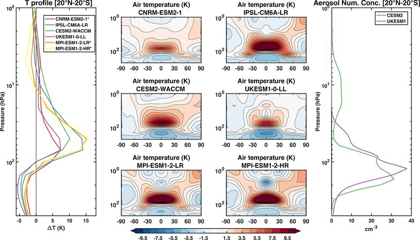
D. Visioni et al.: Identifying the sources of uncertainty in climate model simulations 10043
(Fig. 1), but the amount of geoengineering required to do
Table 2. Summary of results for the simulations in this work for the last two decades of the experiment (2081–2100). When applicable, values are considered as a global mean, ensemble
mean averages. In the last three columns, the solar reduction needed in the G1 experiment (Kravitz et al., 2021) to offset the forcing of a 4× CO2 increase, the effective equilibrium
so varies across models. There are a variety of overlap-
ping mechanisms that contribute to these differences. As re-
ported in Table 2, the models produce a large spread in the
projected warming produced by the two scenarios. Similar
inter-model spreads have been reported in the recent liter-
TCR (K)
2.0
1.9
2.3
1.8
1.7
2.8
ature for CMIP6 models for both effective equilibrium cli-
mate sensitivity (ECS; the equilibrium warming for a dou-
bling of CO2 ; see Zelinka et al., 2020) and transient cli-
mate response (TCR; the temperature warming with a dou-
ECS (K)
Zelinka et al. (2020)
4.68
4.79
4.56
2.98
2.98
5.36
2.1 ± 0.4
bling of CO2 in a scenario with a 1 % per year CO2 in-
climate sensitivity (ECS) from Zelinka et al. (2020) and the transient climate response (TCR) from Meehl et al. (2020) are included for comparison.
crease; see Meehl et al., 2020). Some models (amongst them
CESM2(WACCM) and UKESM1-0-LL, also present in this
study) have been found to have values well above previously
established likely ranges for both ECS and TCR (Gettelman
et al., 2019; Sherwood et al., 2020). Some of the relation-
ships between the variables reported in Table 2 are explored
Solar reduction (G1)
(%; Kravitz et al., 2021)
4.91
3.72
4.10
4.57
n/a
3.80
4.22 ± 1.00
in Fig. 2. A weak relationship between the different warm-
ing in the SSP scenarios and ECS and TCR is to be expected
due to differences in both the timescale of the response and
the differences in, for instance, other GHGs and tropospheric
aerosols (Hansen et al., 2005) that affect the climate in the
short term and that are not factored in the long-term response
to CO2 changes. For instance, CNRM-ESM2-1 reported an
ECS of 4.79 K (Zelinka et al., 2020) (the second highest here)
Solar reduction (G6)
(%)
2.33
1.36
1.78
2.15
2.15
2.18
1.99 ± 0.36
but a 1T of 1.9 K (the third lowest).
This implies that even if different models agreed on how
much either stratospheric AOD or reduction of the solar con-
stant would be needed to cool globally by 1 K (the efficacy
of the geoengineering method), the overall reported amount
of intervention needed would be different due to the differ-
ent response to the forcing from CO2 . To first order, there
(Tg-SO2 /yr)
29 ± 9
Injected SO2
21a
n/ab
40a
36b
36b
21a
should be no expectation that the sensitivity of climate mod-
els to a CO2 increase should be related to the reduction in
temperature due to geoengineering (Kravitz et al., 2021), and
a Models using emissions of SO . b Models using prescribed AOD. n/a – not applicable
we indeed show this in Fig. 2. In Fig. 2f we show that nor-
malizing the required solar dimming or produced AOD in
AOD
0.296
0.327
0.363
0.235
0.235
0.357
0.307 ± 0.061
the last two decades to the global cooling in the same pe-
riod slightly increases the inter-model spread from 19.9 %
to 22.8 % for solar dimming and from 17.2 % to 20.7 % for
AOD compared to the mean (the same quantities, not normal-
ized, are shown in Fig. S1 in the Supplement). In Fig. 2e we
1T (K)
(SSP58.5-SSP24.5)
2.42
1.90
2.40
1.58
1.50
2.54
2.05 ± 0.42 K
also show that the amount of solar reduction and the globally
averaged stratospheric AOD seem to be only weakly related
(R 2 = 0.72), suggesting that there are different mechanisms
involved in the cooling due to the aerosols and the cooling
due to reduced insolation. For G6sulfur, this might be due
not only to the radiative treatment of the aerosols themselves
2
but also to different latitudinal distribution in AOD resulting
CESM2(WACCM)
in different forcing compared to the broad solar reduction
MPI-ESM1.2-HR
MPI-ESM1.2-LR
IPSL-CM6A-LR
CNRM-ESM2-1
UKESM1-0-LL
that is nearly spatially identical in all models.
Model average
The time-dependent amount of geoengineering needed in
all models for the two experiments is reported in Fig. 3a–
Model
b, together with the top-of-atmosphere (TOA) forcing im-
balance between SSP5-8.5 and SSP2-4.5, calculated as the
https://doi.org/10.5194/acp-21-10039-2021 Atmos. Chem. Phys., 21, 10039–10063, 2021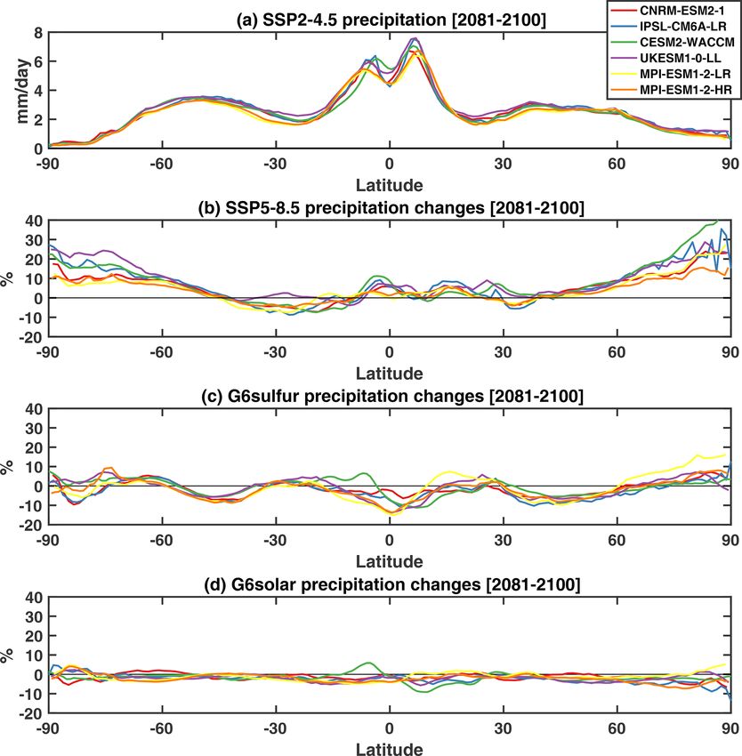
10044                                   D. Visioni et al.: Identifying the sources of uncertainty in climate model simulations

Figure 1. Global mean surface temperatures (◦ C) for the four experiments for each participating model. Single ensemble realizations are
shown in lighter lines, while the ensemble mean is shown in thicker lines. The multi-models mean is shown at the bottom, with the shading
representing 1σ standard deviation of the mean for each experiment.

incoming minus the outgoing longwave and shortwave radi-               in larger differences in the first years. Later in the century,
ation (Fig. 3c), and the underlying difference in CO2 con-             when the temperature difference is larger and the interven-
centration, common to all models, as prescribed for the SSP            tion scales up, inter-model differences may be explained by
scenarios in Meinshausen et al. (2020) (Fig. 3d). In terms             the presence of non-linearities or other effects (such as an in-
of TOA forcing, models show a more consistent forcing that             crease in stratospheric water vapor; Visioni et al., 2017a). It
is a result, mostly, of the same CO2 increase, but they dis-           is interesting to note that while a large portion of the models
agree both in the magnitude of the warming produced by this            do not vary the amount of geoengineering smoothly, but once
same forcing (as shown in Fig. 1) and in the amount of in-             a decade, the applied step function is not evident in the glob-
tervention (optical depth or solar reduction) needed to over-          ally averaged surface temperature responses shown in Fig. 1,
come that forcing, as shown in Fig. 3a and b. The compar-              where there is no qualitative difference between models in
ison between the two forcings is also useful to understand             terms of decadal variability. Since it is similarly present in
the behavior of the geoengineering amount in the models                the G6solar experiments, the reason for this may be found
in the first 30 years, where most models indicate little to            in the slower oceanic response. Future analyses should in-
no geoengineering is necessary. CESM2-WACCM is an ex-                  vestigate whether the step function introduced by some of
ception, and indeed shows a slight overcooling in the first            the models results in changes in surface climate that, while
decades compared to other models; this is most likely a fea-           hidden when considering global or decadal averages, might
ture of the current feedback controller, as has been observed          be present when looking at particular regions or climate fea-
in Tilmes et al. (2018a). The algorithm, which decides how             tures (for instance, the monsoon season) in the years where
much to inject each year by learning from past years, re-              the step change is present.
quires some time to properly converge before it can success-
fully determine the necessary amount. More generally, the              3.2   Differences in the stratospheric response
small differences between the two underlying scenarios in
terms of global mean temperature in the first three decades            For the G6sulfur simulations, the global mean AOD is not, on
tend to magnify small differences in the required interven-            its own, enough to understand the different models’ behav-
tion, as manually estimated by the modeling teams, resulting           ior. Different spatial distributions of the aerosol layer, while
                                                                       yielding similar global values, might result in different ef-

Atmos. Chem. Phys., 21, 10039–10063, 2021                                               https://doi.org/10.5194/acp-21-10039-2021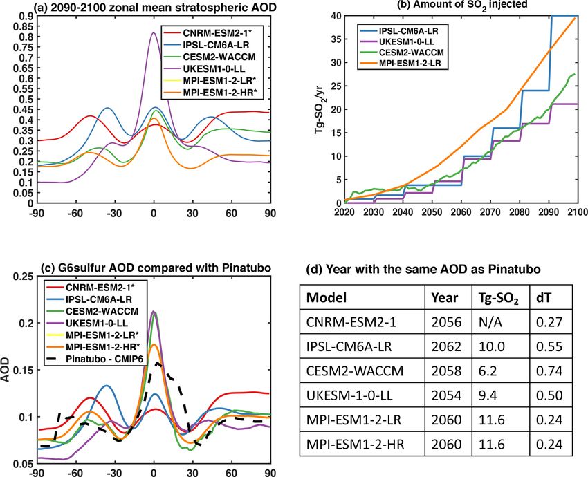
D. Visioni et al.: Identifying the sources of uncertainty in climate model simulations                                               10045

Figure 2. (a–e) Scatter plot of various relationships between some global quantities in the participating models. 1T is between SSP5-8.5 and
SSP2-4.5, and global stratospheric aerosol optical depth (SAOD) and solar reduction are defined in the 2081–2100 period. Transient climate
response (TCR) and effective equilibrium climate sensitivity (ECS) are taken from Zelinka et al. (2020) and Meehl et al. (2020). The R 2 and
the slope of the linear fit (m) are shown for each panel. (f) Values in panels (c)–(d) are normalized by the 1T in the same model to obtain
the normalized intervention (green for solar dimming and orange for stratospheric AOD) needed to cool by 1 K, with multi-model average
on the right and error bars indicating the standard error.

ficiency and would produce different responses of the sur-              2021). The response to the presence of the aerosols them-
face climate (MacMartin et al., 2017; Kravitz et al., 2019;             selves can in turn produce differences in stratospheric dy-
Visioni et al., 2020b). Reasons for a different aerosol dis-            namics, for instance, interacting with the quasi-biennial os-
tribution with similar injection locations and height of SO2            cillation (Aquila et al., 2014; Richter et al., 2017), strength-
can be the different dynamical features of the simulated                ening the tropical confinement of the aerosols (Niemeier and
stratosphere and/or differences in the aerosol microphysics             Schmidt, 2017; Visioni et al., 2018b).
schemes (Pitari et al., 2014; Niemeier et al., 2020; Franke                Furthermore, even given similar annually averaged AOD
et al., 2021) resulting in different aerosol growth, transport          distributions, differences in the seasonal cycle might lead to
and sedimentation, as already shown for simulations of ex-              different surface climate (Visioni et al., 2020b). The spatial
plosive volcanic eruptions (Marshall et al., 2018; Clyne et al.,        distributions of AOD for the last decade of the experiment

https://doi.org/10.5194/acp-21-10039-2021                                               Atmos. Chem. Phys., 21, 10039–10063, 2021
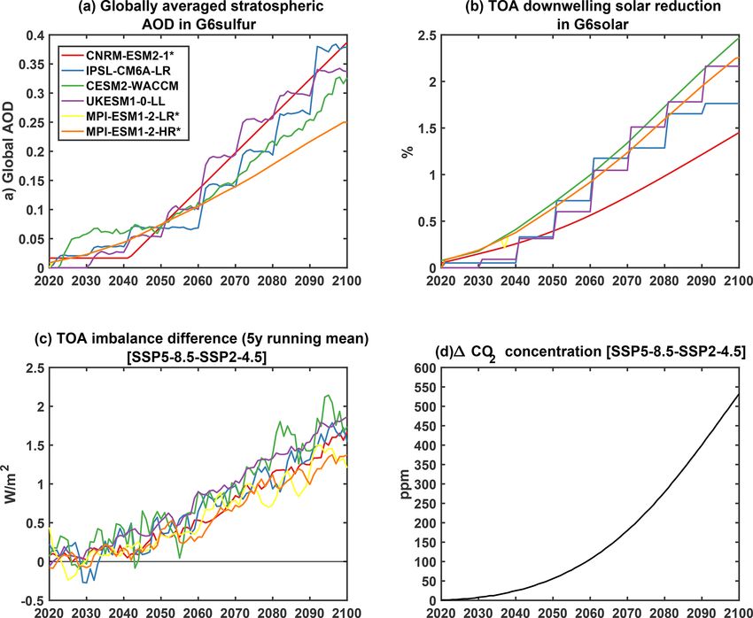
10046                                     D. Visioni et al.: Identifying the sources of uncertainty in climate model simulations

Figure 3. Time-dependent evolution for all participating models of (a) globally averaged stratospheric AOD increase in the G6sulfur ex-
periment (models with an asterisk in the legend have prescribed AOD and the orange and yellow line for the two MPI-ESM1-2 versions
completely overlap); (b) solar reduction in the G6solar experiment as a fraction of the overall incoming solar radiation; (c) top-of-atmosphere
radiative forcing imbalance (downwelling solar radiation minus upwelling solar+longwave radiation) difference between the two baseline
SSP scenarios; and (d) difference in CO2 concentration between the two emission scenarios from Meinshausen et al. (2020) presented for
reference.

in each model are shown in Fig. 4a. Results vary widely be-               servational support, resulting in a narrow spread that might
tween models: UKESM1-0-LL represents a clear outlier in                   be inaccurate, or the spread might be large because some
the tropics, with more than twice the sulfate AOD as other                model results are simply inconsistent with available obser-
models. At high latitudes, on the other hand, there is a much             vations. Here, we try to better constrain the distribution of
larger inter-model spread, with values ranging from 0.1 to 0.3            AOD in the various models in G6sulfur using the up-to-date
at 90◦ S and from 0.2 to 0.45 at 90◦ N. Strong disagreement               CMIP6 dataset for volcanic forcing that combines measure-
between model-simulated AOD in a geoengineering scenario                  ments from various sources (Dhomse et al., 2020; retrieved
was already reported in Pitari et al. (2014) and Plazzotta et al.         from ftp://iacftp.ethz.ch/pub_read/luo/CMIP6/, last access:
(2018) for the G4 experiments, where a 5 Tg-SO2 /yr injec-                29 October 2020). In particular, using the 550 nm extinc-
tion in the equatorial stratosphere was prescribed in the sim-            tion data, we derive the stratosphere-only latitudinal distribu-
ulation protocols. No models used in that experiment have                 tion of the optical depth following the Pinatubo 1991 erup-
been used in the G6 scenarios, so a direct comparison can’t               tion, averaged from 1 month after the eruption (July 1991)
be done with different versions of the same models. In this               to 1 year after in order to also consider the poleward trans-
case, however, we can note that all models at least agree on              port of the aerosols. It needs to be highlighted that the com-
the presence of a confinement of a portion of the aerosols in             parison between an impulsive injection (as Pinatubo) versus
the tropical pipe, whereas in G4 half of the models reported              a sustained injection (as in the geoengineering experiment)
much less AOD in the tropics and more at very high latitudes              is an imperfect one, both in terms of the aerosol distribu-
(Pitari et al., 2014), which is physically very unlikely given            tion and in terms of the effects on surface climate (Duan
observations from the Pinatubo eruption in 1991 (Robock,                  et al., 2019), but it is possibly the only “real”, albeit im-
2000; Pitari et al., 2016).                                               perfect, point of comparison between model behavior and
   Model spread on a particular result is not, of course, the             the actual atmospheric behavior. In the case of a volcanic
same as uncertainty; models may agree despite a lack of ob-               eruption, the precise meteorological conditions strongly in-

Atmos. Chem. Phys., 21, 10039–10063, 2021                                                   https://doi.org/10.5194/acp-21-10039-2021
D. Visioni et al.: Identifying the sources of uncertainty in climate model simulations                                      10047

fluence the resulting AOD; furthermore, the SO2 is injected       (2013) found a cooling of 0.14 K when considering the At-
in a clean stratosphere. Therefore, the following compari-        lantic multidecadal variability. The multi-model average for
son should not be considered as a way of measuring which          the G6sulfur simulation is very similar to the higher esti-
model is closer to observations but just as a way to com-         mates, at 0.46 K ± 0.09, but there is a large range in the single
pare the different models when they reach a similar global        values from 0.24 (in MPI-ESM1-2-LR) to 0.74 (for CESM2-
AOD. In Fig. 4c we report the AOD from Pinatubo derived           WACCM). The two global coolings could be hard to com-
this way and we then compare the results with those from the      pare, however, due to their different nature (impulsive versus
various G6sulfur models. To do so, we consider the year in        sustained). Overall, the comparisons shown in Fig. 4 raise
which each model reaches the same global value of AOD as          an important point that should be taken into account when
Pinatubo and plot the latitudinal distribution of AOD for each    analyzing G6 simulations in future work. While limiting the
model in that year. This comparison highlights various ele-       analyses towards the end of the century might yield a higher
ments that would be lost considering the results towards the      signal-to-noise ratio, it also risks magnifying uncertainties
end of the century as in Fig. 4a. Models show a higher agree-     related to non-linear processes in the stratosphere. In Fig. S2
ment considering a moderate level of global AOD reached           in the Supplement, we also report the yearly evolution of the
and, compared with the results from Pinatubo (considering         latitudinal distribution of AOD for models that inject SO2 ,
the differences in meteorology and injection location), they      normalized by the amount of SO2 injected in that year, which
look reasonable. In particular, UKESM1-0-LL and CESM2-            clearly shows the decrease in efficiency at higher injection
WACCM show a better agreement in their tropical AOD, as           loads.
opposed to what was shown in Fig. 4a, indicating the pres-           As mentioned before, the presence of aerosols in the
ence of non-linearities at high injection rates that might be     stratosphere also produces a perturbation of stratospheric
induced in UKESM1-0-LL by a too strong confinement of             dynamics (Richter et al., 2017; Visioni et al., 2020a) that,
the aerosols in the tropical pipe as a consequence of the dy-     in turn, might affect precipitation (Simpson et al., 2019)
namic response to heating (Aquila et al., 2014; Niemeier and      and temperature (Jiang et al., 2019) at the surface. The re-
Schmidt, 2017; Visioni et al., 2018b). In Fig. 4c, models         sponse is driven by the absorption of infrared radiation by
also show a much better agreement at high latitudes (at least     the aerosols resulting in the heating of the stratospheric air
in the Northern Hemisphere) compared to Fig. 4a, with the         and is thus dependent on the overall burden and the size of
exception of the prescribed AOD in CNRM-ESM2-1. This              the particles (Pitari et al., 2016) but also on interactions with
suggests that when considering higher injection loads, there      the chemical cycles in the stratosphere (Visioni et al., 2017b;
could be a stronger interaction of the produced dynamical         Richter et al., 2017) and the incursion of water vapor from
changes with the simulated AOD at high latitudes (Visioni         the troposphere due to the warming of the tropopause layer
et al., 2020a).                                                   (Visioni et al., 2017b; Tilmes et al., 2018b; Boucher et al.,
   The amount of SO2 needed to reach a certain strato-            2017). In Fig. 5 we show the stratospheric temperatures in the
spheric AOD varies considerably between climate models            last two decades of the G6sulfur experiment for all models.
with interactive stratospheric aerosols even for simulations      Interestingly, the model with the highest AOD in the tropics,
of Pinatubo, ranging in current estimates between 10 and          UKESM1-0-LL, is also one of the models showing the least
20 Tg-SO2 with a central value of 14 (Timmreck et al.,            amount of stratospheric heating, whereas IPSL-CM6A-LR,
2018). In the G6sulfur experiments, the models show dis-          with an average tropical AOD (but much larger SO2 injec-
crepancies in the estimate of the amount needed to achieve        tion needed to achieve it) shows a temperature change that
a similar global AOD as in Pinatubo (with a multi-model           is much larger than the others. The reasons for this may de-
average of 9.3 ± 2.3 Tg-SO2 ; see table in Fig. 4), closer to     pend on multiple aspects that would need to be investigated
the lower limit from Timmreck et al. (2018) (10 Tg-SO2 )          separately. For instance, the reasons might include that there
for UKESM1-0-LL and IPSL-CM6A-LR and 60 % lower                   are different size distributions of the stratospheric aerosols,
for CESM2-WACCM. For CESM2-WACCM, the difference                  different concentrations of particles (shown in Fig. 5), dif-
could be partially explained by the difference in altitude for    ferences in ozone changes resulting in different heating rates
the SO2 injections. In Fig. 4c we also report the cooling pro-    (Richter et al., 2017; Niemeier et al., 2020), different heating
duced by the G6sulfur aerosols, compared to SSP5-8.5 in the       from stratospheric water vapor (Pitari et al., 2014; Simpson
considered year (we used a 5-year average around that year to     et al., 2019) or differences in the radiative schemes between
reduce the contribution of natural variability). For Pinatubo,    models.
there is uncertainty in the cooling produced by the volcanic
aerosols due to the precise meteorology of that year (for in-     3.3   Surface climate response
stance, the influence of an El-Niño event or other climatic
oscillations compared to the years immediately before/after);     When geoengineering the climate, reducing incoming solar
Parker et al. (1996) estimate a global cooling of around 0.4 K,   radiation (either by simulating stratospheric aerosols or by
and similarly Soden et al. (2002) estimated a range between       reducing the solar constant in models) to obtain the same
0.3 and 0.5 K, whereas more recent estimates by Canty et al.      global surface temperature as a scenario with lower GHGs

https://doi.org/10.5194/acp-21-10039-2021                                       Atmos. Chem. Phys., 21, 10039–10063, 2021
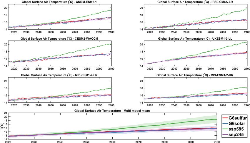
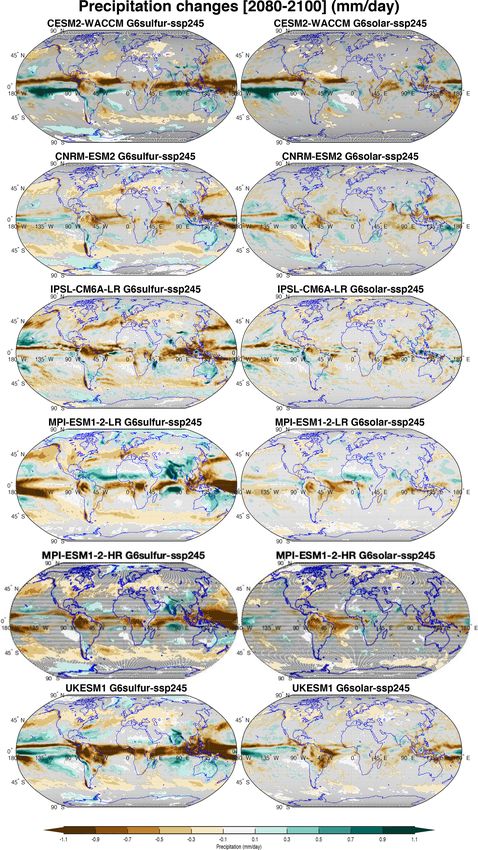
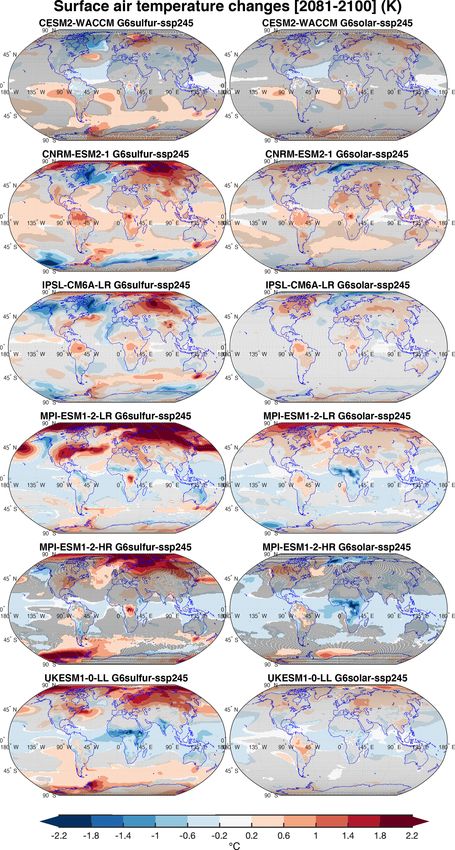
10048                                    D. Visioni et al.: Identifying the sources of uncertainty in climate model simulations

Figure 4. (a) Stratospheric AOD in the last decade of the experiment for all participating models. The asterisk in the legend indicates models
with prescribed optical depth. (b) Injected SO2 for available models in Tg-SO2 /yr. (c) AOD distribution for each model in the year with a
global AOD closest to that from Pinatubo (0.102, averaged from July 1991 to June 1992) and comparison with the latitudinal distribution
for the volcanic eruption following the new CMIP6 composed dataset (Dhomse et al., 2020). (d) The year where the global value of AOD
reaches 0.102 in the model is indicated, together with the amount of SO2 needed to achieve that value and the cooling produced in G6sulfur
compared to SSP5-8.5 in that year. Models marked with an asterisk in the legend used prescribed aerosol distributions for G6sulfur. The
orange and yellow lines for the two MPI-ESM1-2 versions always overlap.

does not assure that regional temperatures follow the same               the ocean circulation. This latter point has been observed,
pattern. This has been reported in climate model simulations             for instance, in CESM1(WACCM) in Fasullo et al. (2018)
of various complexity, from 1-D models (Henry and Merlis,                and in one of the models that performed G6 simulations,
2020) to Earth system model simulations (i.e., Ban-Weiss                 CESM2(WACCM), in Tilmes et al. (2020).
and Caldeira, 2010; Niemeier et al., 2013; Jones et al., 2018;              All of these differences are compounded with those al-
Visioni et al., 2021). These differences may be reduced if,              ready present in climate models for regional temperature pro-
together with reducing global temperatures, the geoengineer-             jections for CO2 increases. On this point, however, Mac-
ing strategy also aims to reduce differences in higher-order             Martin et al. (2015) argued that reducing surface tempera-
temperature gradients (Kravitz et al., 2016; Tilmes et al.,              tures through geoengineering has the potential to actually re-
2018a), but they cannot be completely canceled due to var-               duce model spread in regional projections. That work, how-
ious factors. The main factor would be a fundamental dif-                ever, considered the G1 experiment, which entails a uniform
ference in the radiative perturbation from CO2 (that warm                solar reduction to reduce temperatures under a 4×CO2 in-
throughout the atmospheric column) and from the reduction                crease. Clearly then, most of the differences listed above are
in solar constant (that cool from the bottom-up)(Ban-Weiss               not included in such an idealized experiment. This is clear
and Caldeira, 2010; Henry and Merlis, 2020); then, seasonal              when looking at the multi-model averages of surface tem-
and latitudinal differences (Govindasamy et al., 2003; Ban-              perature differences shown in Fig. 6. The simulated differ-
Weiss and Caldeira, 2010; Visioni et al., 2020b) and surface             ences with SSP2-4.5 are much larger in G6sulfur compared
climate effects (such as precipitation changes) of the strato-           to G6solar and the inter-model spread is also much larger
spheric heating produced by the aerosols (Simpson et al.,                in G6sulfur. This indicates that there is better agreement be-
2019; Visioni et al., 2021; Jones et al., 2021). Other fac-              tween models when the uncertainties related to the strato-
tors may also be an inability to restore the same state for              spheric sulfate are removed. For G6sulfur, there is a general

Atmos. Chem. Phys., 21, 10039–10063, 2021                                                  https://doi.org/10.5194/acp-21-10039-2021
D. Visioni et al.: Identifying the sources of uncertainty in climate model simulations                                              10049

Figure 5. Profile of stratospheric temperature changes (G6sulfur minus SSP5-8.5) between 20◦ N and 20◦ S are shown in the left panel. In
the central panels, the changes are shown for each participating model. The profiles of aerosol number concentration are shown in the right
panel for a select number of models where output was available. All changes are for the years 2081–2100 and evaluated against the same
period for the underlying emission scenario SSP5-8.5.

agreement in the inability of sulfate geoengineering to com-            which some observations can be made that would not be
pletely cool down the northern high latitudes, partly due to            immediately evident from the multi-model average. For
the focus of the geoengineering strategy on reducing global             G6sulfur, there is good agreement regarding the residual
mean temperatures (Kravitz et al., 2019) but also probably              warming over northern Eurasia across models, with the ex-
due to the presence of stratospheric heating (Jiang et al.,             ception of CESM2. There is less agreement over North
2019), as evident by the absence of high-latitude warming               America, where some models simulate a cooling in G6sulfur
with the same magnitude in the G6solar simulations. The                 compared to SSP2-4.5 while some simulate a warming. This
residual warming also present in the G6solar simulations can            might be due to differences in the response of the North At-
be partly explained by the differences in the radiative forcing         lantic circulation both to increasing GHGs and to geoengi-
from the CO2 and solar reduction (Ban-Weiss and Caldeira,               neering (Tilmes et al., 2018a, 2020). Comparing this result to
2010; Henry and Merlis, 2020; Visioni et al., 2021). Differ-            that from G6solar, where there is a concurrence of all models
ences in the surface response between models would thus de-             in simulating a small warming over the same region, could
pend on how different models physically reproduce some of               indicate that the much different response in G6sulfur might
the processes mentioned but also on the differences in the              on the other hand be due to differences in the distribution
stratospheric response reported in the previous section. Dif-           of the stratospheric aerosols. UKESM1-0-LL, for instance,
ferent latitudinal and seasonal distributions of the aerosols           where more residual warming is present, shows the lowest
produce different climate states even in the same model (as             AOD over high latitudes (Fig. 4). In the tropics, the Amazon
shown in CESM1(WACCM) in Kravitz et al., 2019; Visioni                  region models seem to differ more in the G6sulfur case and
et al., 2020b), and the stratospheric heating is also report-           less in the G6solar case; possible causes might be an influ-
edly different, as shown in Fig. 5. Nonetheless, the essential          ence from the different magnitude of AOD in that region, dif-
finding from MacMartin et al. (2015) still holds when com-              ferent responses of the vegetation to increasing CO2 concen-
paring the multi-model standard error for the geoengineering            trations and reduced solar radiation (Simpson et al., 2019) or
projections against those for the SSP5-8.5 changes: that espe-          local changes in atmospheric circulation (Jones et al., 2018).
cially over land and at high latitudes inter-model differences             Overall, the inter-model differences indicate the need for
are always higher than both G6 cases.                                   some care when trying to understand the possible surface im-
   We report the surface temperature maps for the last two              pacts of sulfate geoengineering by using multi-model ensem-
decades of the experiment for each model in Fig. 7, from                bles. It might be difficult to correctly separate the differences

https://doi.org/10.5194/acp-21-10039-2021                                              Atmos. Chem. Phys., 21, 10039–10063, 2021
10050                                      D. Visioni et al.: Identifying the sources of uncertainty in climate model simulations

Figure 6. (a, c, e) Multi-model averages for surface temperature changes averaged over 2081–2100 in different cases: (a) SSP5-8.5,
(c) G6sulfur, and (e) G6solar minus the same period for SSP2-4.5. Etched areas (in gray) indicate where less than 66 % of the models
(here, four out of six) agree on the sign of the difference in that grid point. Note the different color bar between panel (a) and panels (c)–(e).
(b, d, f) Standard error in the multi-model mean for the same reference case on the left. All model results have been re-gridded using a
common grid equivalent to that from the model with the lowest horizontal resolution.

in surface impacts due to differences in the stratospheric                 tica case), as also shown in McCusker et al. (2015), and that
AOD (shown in Fig. 4) given a similar injection and those                  this might be model dependent (other than being dependent
produced by different response of the surface climate. While               on the particular injection strategy) or due to a different re-
comparing results with those from a similar, more uniform                  sponse of the atmospheric circulation (Jones et al., 2018). On
experimental design such as G6solar might help, the lack                   the other hand, parts of the response, such as the patches of
of the potential response produced by the aerosols (Banerjee               warming present in the Amazon and in Central Africa, pos-
et al., 2021; Visioni et al., 2021) may suggest the use of a pre-          sibly due to a different land response, are shared between the
scribed aerosol distribution for various models (Tilmes et al.,            two versions and similarly a large part of the warming over
2015) as an intermediate approach. This can also be seen in                Eurasia. While observing the response of different versions
the comparison between the two versions of MPI (that differ                of the same model to the same forcing might point to some
only in their horizontal resolution, which is twice as high in             of the causes, comparing that to the response of a different
the HR version). They both use the same AOD distribution                   model to the same forcing may also highlight which parts of
and have the same magnitude of stratospheric AOD in the                    the overall response is model dependent and which are robust
whole period. Yet, they show some considerable differences                 across models.
in the surface temperature response to the same aerosol (or                   Surface temperatures are not the only measure of the
even solar) forcing. In particular, the warming observed over              possible impacts of either climate change or geoengineer-
North America in the LR version is not as high in the HR                   ing; amongst the many others, hydrological cycle changes
version, whereas the warming present in West Antarctica in                 are also central to any assessment. Under climate change,
the HR version is not present in the LR version. This might                due to the surface and tropospheric warming allowing for
indicate that the regional temperature response is due to a dif-           more moisture to be retained by the air, global precipita-
ferent deep ocean circulation response (in the West Antarc-                tion has been consistently projected to increase (Pendergrass

Atmos. Chem. Phys., 21, 10039–10063, 2021                                                     https://doi.org/10.5194/acp-21-10039-2021
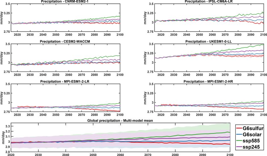
D. Visioni et al.: Identifying the sources of uncertainty in climate model simulations                                                10051

Figure 7. Surface temperatures changes in the period 2081–2100 in G6sulfur compared to the same period for SSP2-4.5 in G6sulfur sim-
ulations (left panels) and G6solar simulations (right panels) for all participating models. Shaded areas indicate where the difference is not
statistically significant, as evaluated using a double-sided t-test with p < 0.05 on the ensemble averages for each model and considering all
20 years as independent samples.

https://doi.org/10.5194/acp-21-10039-2021                                               Atmos. Chem. Phys., 21, 10039–10063, 2021
10052                                  D. Visioni et al.: Identifying the sources of uncertainty in climate model simulations

Figure 8. Global mean precipitation (mm/day) for the four experiments for each participating model. The multi-models mean is shown at
the bottom, with the shading representing 1σ standard deviation of the mean for each experiment.

and Hartmann, 2014) and a similar behavior is displayed              compensation and in the difference between G6solar and
by the models participating in the G6 experiments (Fig. 8).          G6sulfur. The fact that under the SSP2-4.5 scenario some
Similarly, it has been widely assessed that trying to restore        warming continues during the 21st century, combined with
surface temperature to a previous state by means of modi-            the precipitation overcompensation by geoengineering, re-
fying the top of the atmosphere radiative balance tends to           sults in some models having no changes in global precipi-
overcompensate the changes in precipitation, therefore re-           tation compared to the beginning of the century (as already
ducing global mean precipitation. Globally, the changes are          noted in Irvine and Keith, 2020); only G6sulfur in IPSL-
driven by the perturbation of the surface heat fluxes (Tilmes        CM6A-LR shows a decrease compared to that period by the
et al., 2013; Kravitz et al., 2013b; Niemeier et al., 2013) and      end of the century. For the purpose of future analyses, the
changes in sea–land temperature contrast. Regionally, how-           anomalous global precipitation response in the MPI models
ever, the modification of the baseline distribution of precip-       for G6sulfur has to be noted. It is very likely that the slightly
itation can be due to changes in the inter-tropical conver-          larger response in global mean precipitation at the beginning
gence zone (ITCZ; Russotto and Ackerman, 2018b; Cheng                of the century is due to differences in the initialization pro-
et al., 2019) produced by changes in the inter-hemispheric           cess for those simulations rather than in a change produced
temperature gradient, general circulation changes produced           by the sulfate (which is very close to zero, in 2020) and re-
by stratospheric heating (Simpson et al., 2019) and regional         sults before 2050 (for the LR version) or 2040 (for the HR
and seasonal changes in heat fluxes and temperature gradi-           version) should not be considered as representative.
ents (Jones et al., 2018; Visioni et al., 2020b). In the case of        From the perspective of assessing ecosystem impacts, this
sulfate injections, these changes can be strongly dependent          decoupling of precipitation, temperatures and CO2 should be
on latitudinal and temporal distribution of the aerosol cloud        investigated in depth to understand if and where it would be
as well (Kravitz et al., 2019; Visioni et al., 2020b).               beneficial or not. It also further stresses the notion that reduc-
   The response of the various models for the G6 experiments         ing precipitation is not an automatic result of geoengineer-
in Fig. 8 consistently shows that the global mean precipi-           ing but that the outcome is related to which specific cooling
tation would be overcompensated (Niemeier et al., 2013).             targets geoengineering is deployed to achieve (Tilmes et al.,
However, models disagree on the magnitude of this over-              2013; Irvine et al., 2019; Lee et al., 2020). All models agree,

Atmos. Chem. Phys., 21, 10039–10063, 2021                                             https://doi.org/10.5194/acp-21-10039-2021
D. Visioni et al.: Identifying the sources of uncertainty in climate model simulations                                                   10053

Figure 9. (a, c, e) Multi-model averages for precipitation changes averaged over 2081–2100 in different cases: (a) SSP5-8.5, (c) G6sulfur,
and (e) G6solar minus the same period for SSP2-4.5. Etched areas (in gray) indicate where less than 66 % of models (here, four out of six)
agree on the sign of the difference in that grid point. (b, d, f) Standard error in the multi-model mean for the same reference case on the left.
All models results have been re-gridded using a common grid equivalent to that from the model with the lowest horizontal resolution.

to various degrees, that global precipitation changes under                WACCM shows less precipitation in the tropical Northern
G6sulfur are larger than the same changes under G6solar.                   Hemisphere and more precipitation in the tropical Southern
There might be various reasons for this, such as differences               Hemisphere, UKESM1-0-LL presents a drying in both hemi-
in latent heat due to different ratios of diffuse solar radia-             spheres, especially over continents. In some cases, such as at
tion (that increases in the case of the sulfate aerosols; Vi-              high northern latitudes, all models show a positive change in
sioni et al., 2021) resulting in more atmospheric absorp-                  G6sulfur and a negative change in G6solar. It is again inter-
tion or changes in cloud formation produced by the differ-                 esting to note the differences in the projected precipitation
ent vertical atmospheric temperature gradient. Niemeier et al.             changes in the two versions of MPI. The HR version shows
(2013) suggested that the reason for this might be found in                both further decreases and increases in precipitation in the
the stratospheric heating produced by the aerosols result-                 tropics compared to the LR version, and at high latitudes LR
ing in more water vapor entering the stratosphere from the                 shows much higher changes compared to HR. This shows
warming of the tropopause layer (Tilmes et al., 2018a; Simp-               that even given the same AOD distribution and similar mod-
son et al., 2019) producing a small positive radiative forcing             els, some of the observed changes in the case of SAI may
whose warming effect (Hansen et al., 2005; Visioni et al.,                 differ depending on the simulated response of the circulation
2017a) needs to be counterbalanced by injecting slightly                   to the same forcing, which in the two versions of MPI could
more aerosols.                                                             be caused by the different horizontal resolution. In this work
   Lastly, models agree on regional precipitation changes                  we have only analyzed the annual response to precipitation,
more in G6solar than in G6sulfur (Fig. 9), but all mod-                    but there are many regions where changes to the seasonal cy-
els project most of the significant changes will occur over                cle of precipitation may be even more crucial, such as those
the tropics (where most of the baseline precipitation is also              that experience a monsoon climate and whose cycle might be
located), although with some significant local differences                 affected by SAI (see, for instance, Simpson et al., 2019; Vi-
between models (Fig. 10). For instance, while CESM2-                       sioni et al., 2020b for the Indian subcontinent, and Da-Allada

https://doi.org/10.5194/acp-21-10039-2021                                                  Atmos. Chem. Phys., 21, 10039–10063, 2021
10054                                     D. Visioni et al.: Identifying the sources of uncertainty in climate model simulations

Figure 10. Precipitation changes (mm/day) in the period 2081–2100 in G6sulfur compared to the same period for SSP2-4.5 in G6sulfur
simulations (left panels) and G6solar simulations (right panels) for all participating models. Shaded areas indicate where the difference is not
statistically significant, as evaluated using a double-sided t-test with p < 0.05 and considering all 20 years as independent samples.

Atmos. Chem. Phys., 21, 10039–10063, 2021                                                   https://doi.org/10.5194/acp-21-10039-2021
D. Visioni et al.: Identifying the sources of uncertainty in climate model simulations                                        10055

                                                                     comparing the global mean versus the land-mean. As this
                                                                     could be due to a variety of factors, future studies should try
                                                                     to elucidate what is causing these different responses in the
                                                                     various models.

                                                                     4   Conclusions

                                                                     We have shown in this work some preliminary results from
                                                                     the G6sulfur and G6solar modeling experiments proposed
                                                                     in Kravitz et al. (2015) for the Geoengineering Model In-
                                                                     tercomparison Project as part of the Climate Model Inter-
                                                                     comparison Project Phase 6. These two new experiments
                                                                     aim to reduce global temperatures in the 21st century from
                                                                     those simulated under a high-tier emissions scenario (SSP5-
                                                                     8.5) to those simulated under a medium-tier emissions sce-
                                                                     nario (SSP2-4.5), either by simulating the artificial injection
                                                                     of stratospheric aerosol precursors in the stratosphere or by
                                                                     reducing the solar constant in the models. In terms of sur-
                                                                     face climate response, some broad features are shared by
                                                                     all models, such as a reduction in global mean precipitation
                                                                     compared to both SSP scenarios and a residual warming in
Figure 11. (a) Zonal mean precipitation (mm/day) in the period
                                                                     the northern high latitudes (Henry and Merlis, 2020), which
2081–2100 in SSP2-4.5. (b) Precipitation changes (%) compared to
SSP2-4.5 in the same period for SSP5-8.5. (c–d) as in (b), but for   is particularly present in G6sulfur (Simpson et al., 2019;
G6sulfur and G6solar, respectively.                                  Banerjee et al., 2021). Other locations show more disagree-
                                                                     ments between models in terms of the surface temperature
                                                                     response. Since there is a larger uniformity in the response
                                                                     between G6solar simulations, where the solar dimming is
et al., 2020 for western Africa); an in depth analyses of these      applied in the same latitudinally uniform way in all mod-
impacts would also be necessary. Interestingly, unlike for the       els, this suggests that part of the surface response uncertainty
surface temperatures multi-model standard error (Fig. 6), the        in G6sulfur is driven by differences in the latitudinal distri-
standard error for precipitation is very similar and in some         bution of the aerosols and not to a different response of the
cases higher in G6sulfur than in SSP5-8.5.                           surface climate to the same radiative forcing.
   This indicates that while it is true that reducing surface           The comparison of the two experiments may help in vari-
temperatures would indeed reduce disagreement in future              ous ways. When comparing the single-model response to the
projections between models, this might not hold true for             two different forcings, it helps highlight some of the physi-
other impacts (of which precipitation might only be an ex-           cal differences between the two interventions (as in Visioni
ample). For them, due to the influence of changes in sur-            et al., 2021) produced by the stratospheric aerosols’ physical
face temperatures, effects driven by CO2 (both radiative             and chemical effects. Analyzing the inter-model spread also
and physiological) and possible changes in dynamical per-            highlights the degree to which uncertainty in surface climate
turbations driven by the aerosols, modeling uncertainties            response to stratospheric aerosols is driven by uncertainties
might remain higher either with high CO2 or with geo-                in the stratospheric processes versus uncertainties in how
engineering. Some of the drivers of uncertainty may be ob-           the climate response to a specified forcing such as reduced
served by looking at global and land mean precipitation              insolation and may point to a path to successfully identify
changes in the last 20 years. For the former, the multi-             and, eventually, reduce some of them. We have shown that
model mean projects an increase of 2.28 ± 0.80 % com-                large inter-model variability remains in the distribution of the
pared to SSP2-4.5 in the same period, while it projects              aerosol after injections of SO2 in the tropical stratosphere as
a decrease of −3.79 ± 0.76 % for G6sulfur (compared to               well as in the temperature response of the stratosphere. As we
−2.07 ± 0.40 % for G6solar). For the latter, the SSP5-8.5            discussed in Sect. 3.2, the resulting latitudinal distribution
increase is 1.53 ± 0.73 %, while for G6sulfur the decrease           of the aerosols given similar injection locations can be due
is −3.96 ± 1.50 %, and −2.35 ± 0.79 % (see Fig. S3 in the            to multiple factors, such as the stratospheric dynamics dif-
Supplement for the results of the single models). For both           ferences regulating the large-scale transport of the aerosols
G6sulfur and SSP5-8.5, the spread of the precipitation re-           and the microphysical differences regulating the oxidation
sponse over land is much larger compared to G6solar, and             of SO2 and the subsequent growth of the aerosols. The in-
depending on the model there are different responses when            teraction between the stratospheric aerosols and the rest of

https://doi.org/10.5194/acp-21-10039-2021                                          Atmos. Chem. Phys., 21, 10039–10063, 2021
You can also read