Effects of prescribed CMIP6 ozone on simulating the Southern Hemisphere atmospheric circulation response to ozone depletion - OceanRep
←
→
Page content transcription
If your browser does not render page correctly, please read the page content below
Atmos. Chem. Phys., 21, 5777–5806, 2021
https://doi.org/10.5194/acp-21-5777-2021
© Author(s) 2021. This work is distributed under
the Creative Commons Attribution 4.0 License.

Effects of prescribed CMIP6 ozone on simulating the Southern
Hemisphere atmospheric circulation response to ozone depletion
Ioana Ivanciu1 , Katja Matthes1,2 , Sebastian Wahl1 , Jan Harlaß1 , and Arne Biastoch1,2
1 GEOMAR       Helmholtz Centre for Ocean Research Kiel, Kiel, Germany
2 Faculty   of Mathematics and Natural Sciences, Christian-Albrechts Universität zu Kiel, Kiel, Germany

Correspondence: Ioana Ivanciu (iivanciu@geomar.de)

Received: 11 July 2020 – Discussion started: 5 October 2020
Revised: 31 January 2021 – Accepted: 5 March 2021 – Published: 19 April 2021

Abstract. The Antarctic ozone hole has led to substantial          Ozone depletion is the primary driver of these historical cir-
changes in the Southern Hemisphere atmospheric circula-            culation changes in FOCI. The austral spring cooling of the
tion, such as the strengthening and poleward shift of the mid-     polar cap in the lower stratosphere in response to ozone de-
latitude westerly jet. Ozone recovery during the twenty-first      pletion is weaker in the simulations that prescribe the CMIP6
century is expected to continue to affect the jet’s strength and   ozone field. We attribute this weaker response to a prescribed
position, leading to changes in the opposite direction com-        ozone hole that is different to the model dynamics and is
pared to the twentieth century and competing with the effect       not collocated with the simulated polar vortex, altering the
of increasing greenhouse gases. Simulations of the Earth’s         strength and position of the planetary wavenumber one. As a
past and future climate, such as those performed for the Cou-      result, the dynamical contribution to the ozone-induced aus-
pled Model Intercomparison Project Phase 6 (CMIP6), re-            tral spring lower-stratospheric cooling is suppressed, lead-
quire an accurate representation of these ozone effects. Cli-      ing to a weaker cooling trend. Consequently, the intensifica-
mate models that use prescribed ozone fields lack the impor-       tion of the polar night jet is also weaker in the simulations
tant feedbacks between ozone chemistry, radiative heating,         with prescribed CMIP6 ozone. In contrast, the differences
dynamics, and transport. In addition, when the prescribed          in the tropospheric westerly jet response to ozone depletion
ozone field was not generated by the same model to which           fall within the internal variability present in the model. The
it is prescribed, the imposed ozone hole is inconsistent with      persistence of the Southern Annular Mode is shorter in the
the simulated dynamics. These limitations ultimately affect        prescribed ozone chemistry simulations. The results obtained
the climate response to ozone depletion. This study investi-       with the FOCI model suggest that climate models that pre-
gates the impact of prescribing the ozone field recommended        scribe the CMIP6 ozone field still simulate a weaker South-
for CMIP6 on the simulated effects of ozone depletion in the       ern Hemisphere stratospheric response to ozone depletion
Southern Hemisphere. We employ a new state-of-the-art cou-         compared to models that calculate the ozone chemistry in-
pled climate model, Flexible Ocean Climate Infrastructure          teractively.
(FOCI), to compare simulations in which the CMIP6 ozone
is prescribed with simulations in which the ozone chemistry
is calculated interactively. At the same time, we compare the
roles played by ozone depletion and by increasing concentra-       1   Introduction
tions of greenhouse gases in driving changes in the Southern
Hemisphere atmospheric circulation using a series of histor-       Anthropogenic emissions of ozone-depleting substances
ical sensitivity simulations. FOCI captures the known effects      (ODSs), in particular chlorofluorocarbons (CFCs), have led
of ozone depletion, simulating an austral spring and sum-          to a steep decline in stratospheric ozone concentrations since
mer intensification of the midlatitude westerly winds and of       the 1980s. The strongest ozone depletion occurred in aus-
the Brewer–Dobson circulation in the Southern Hemisphere.          tral spring above Antarctica. There, the particularly low tem-
                                                                   peratures inside the winter polar vortex enable the forma-

Published by Copernicus Publications on behalf of the European Geosciences Union.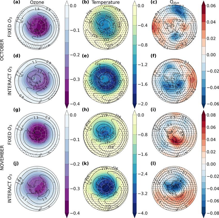
5778                       I. Ivanciu et al.: Effects of CMIP6 O3 on SH atmospheric circulation response to O3 depletion

tion of polar stratospheric clouds (PSCs). Upon the arrival        ozone hole formation include the elevation of the SH po-
of sunlight in spring, heterogeneous chlorine photochem-           lar tropopause (Son et al., 2009; Polvani et al., 2011) and
istry on the surface of PSCs makes chlorine particularly ef-       the poleward expansion of the Hadley cell (Garfinkel et al.,
fective at destroying ozone (e.g., Solomon, 1999). As a re-        2015; Waugh et al., 2015; Polvani et al., 2011; Min and
sult, the ozone hole develops every spring in the Antarctic        Son, 2013; Previdi and Polvani, 2014) in austral summer.
stratosphere, with profound impacts for the Southern Hemi-         The wind stress over the Southern Ocean, associated with
sphere (SH) climate. Observations (e.g., Randel and Wu,            the westerlies, has also experienced a significant strengthen-
1999; Thompson and Solomon, 2002; Randel et al., 2009;             ing and poleward shift (Yang et al., 2007; Swart and Fyfe,
Young et al., 2013) and model simulations (Mahlman et al.,         2012), with implications for the SH ocean circulation. Ocean
1994; Arblaster and Meehl, 2006; Gillett and Thompson,             circulation changes due to the formation of the Antarctic
2003; Stolarski et al., 2010; Perlwitz et al., 2008; Son et al.,   ozone hole include the intensification and poleward shift of
2010; McLandress et al., 2010; Polvani et al., 2011; Young         the SH supergyre, which connects the subtropical Pacific, At-
et al., 2013; Eyring et al., 2013; Keeble et al., 2014) con-       lantic, and Indian Ocean (Cai, 2006), an increase in the trans-
sistently show a cooling of the Antarctic lower stratosphere       port of salty and warm waters from the Indian into the At-
in austral spring and summer during the last decades of the        lantic Ocean, known as the Agulhas leakage (Biastoch et al.,
twentieth century due to decreased radiative heating as a re-      2009, 2015; Durgadoo et al., 2013), and changes in the Ek-
sult of ozone depletion. This cooling has led to important         man transport and upwelling in the Southern Ocean (Thomp-
changes in the dynamics of the SH. Lower polar cap temper-         son et al., 2011, and references therein).
atures resulted in an increased meridional temperature gradi-         As ozone depletion had such profound implications for
ent between the cold polar cap and the relatively warmer mid-      the SH climate, accurate model simulations of past and fu-
latitudes. Consequently, the spring stratospheric polar vor-       ture climate change require a correct representation of strato-
tex strengthened (Thompson and Solomon, 2002; Gillett and          spheric ozone changes and their associated impacts. Multi-
Thompson, 2003; Arblaster and Meehl, 2006; McLandress              ple lines of evidence suggest that the method used to specify
et al., 2010; Thompson et al., 2011; Keeble et al., 2014),         stratospheric ozone in models affects their response to ozone
and its breakdown was delayed by about 2 weeks (Waugh              depletion (Gabriel et al., 2007; Crook et al., 2008; Gillett
et al., 1999; Langematz et al., 2003; McLandress et al., 2010;     et al., 2009; Waugh et al., 2009; Haase and Matthes, 2019).
Previdi and Polvani, 2014; Keeble et al., 2014). This en-          Ozone concentrations can be calculated interactively (e.g.,
abled an intensification of the planetary wave activity prop-      Haase and Matthes, 2019), as is the case in chemistry climate
agating into the stratosphere, resulting in an enhancement         models (CCMs), or they can be prescribed either as zonal
of the Brewer–Dobson circulation (BDC) in austral summer           means, three-dimensionally (3D; e.g., Crook et al., 2008), as
(Li et al., 2008, 2010; Oberländer-Hayn et al., 2015; Polvani      monthly means, or at daily resolution. Ozone asymmetries,
et al., 2018; Abalos et al., 2019).                                the temporal resolution of the prescribed ozone field, and
   At the same time, the strengthening of the stratospheric        feedbacks between ozone, temperature, dynamics, and trans-
westerlies extended downward, affecting the tropospheric jet,      port all impact the way in which changes driven by decreas-
which intensified with a lag of 1 to 2 months in austral sum-      ing ozone concentrations are simulated. This paper investi-
mer (Thompson and Solomon, 2002; Gillett and Thomp-                gates how prescribing the ozone field recommended for the
son, 2003; Perlwitz et al., 2008; Son et al., 2010; Eyring         Coupled Model Intercomparison Project Phase 6 (CMIP6)
et al., 2013). The intensification of the stratospheric and        affects the atmospheric circulation response to ozone deple-
tropospheric jets was accompanied by a concurrent posi-            tion by drawing a comparison with simulations that calculate
tive trend in the Southern Annular Mode (SAM; Thompson             the ozone chemistry interactively.
and Solomon, 2002; Gillett and Thompson, 2003; Marshall,              The position of the Antarctic ozone hole is not centered
2003; Perlwitz et al., 2008; Fogt et al., 2009; Thompson et al.,   above the South Pole but varies with that of the polar vortex,
2011). The surface westerlies strengthened on their pole-          being displaced towards the Atlantic sector in the climatolog-
ward side and weakened on their equatorward side, therefore        ical mean (e.g., Grytsai et al., 2007). As a result, the ozone
shifting towards higher latitudes during the austral summer        field is characterized by asymmetries in the zonal direc-
(Polvani et al., 2011). This resulted in the poleward displace-    tion, henceforth referred to as zonal asymmetries in ozone or
ment of the SH storm track and led to changes in cloud cover       ozone waves. The effect of zonal asymmetries in ozone was
(Grise et al., 2013) and precipitation, not only at the high       previously investigated for both hemispheres (e.g., Gabriel
latitudes and midlatitudes (Polvani et al., 2011; Previdi and      et al., 2007; Crook et al., 2008). In the Northern Hemisphere
Polvani, 2014), but also in the subtropics (Kang et al., 2011).    winter, zonally asymmetric ozone alters the structure of the
The formation of the ozone hole also affected the Antarc-          stationary wave one, resulting in temperature changes in the
tic surface temperatures, with large regional variations in        stratosphere and mesosphere (Gabriel et al., 2007; Gillett
the temperature trend over the continent. Significant warm-        et al., 2009). Ozone waves were also found to affect the num-
ing over the Antarctic Peninsula and Patagonia was reported        ber of sudden stratospheric warmings (SSWs), but studies
by Thompson and Solomon (2002). Other consequences of              disagree about the sign of the change (Peters et al., 2015;

Atmos. Chem. Phys., 21, 5777–5806, 2021                                             https://doi.org/10.5194/acp-21-5777-2021
I. Ivanciu et al.: Effects of CMIP6 O3 on SH atmospheric circulation response to O3 depletion                                 5779

Haase and Matthes, 2019). Peters et al. (2015) reported an          stratospheric temperature and the austral summer strato-
increased number of SSWs and a weakening of the Arctic              spheric westerly jet between simulations with prescribed and
Oscillation between the mid-1980s and mid-1990s in a sim-           interactive ozone.
ulation with specified zonal asymmetries in ozone compared             Feedbacks between stratospheric ozone, temperature, and
to one in which zonal mean ozone was prescribed. In con-            dynamics can only occur in models that calculate the ozone
trast, Haase and Matthes (2019) found that fewer SSWs oc-           chemistry interactively, i.e., in CCMs. The importance of
curred between 1955 and 2019 when zonal asymmetries in              such feedbacks in both hemispheres was previously shown
ozone were prescribed, and even fewer SSWs occurred when            in studies by Haase and Matthes (2019), Haase et al. (2020),
the ozone chemistry was calculated interactively. In a recent       and Oehrlein et al. (2020). Changes in temperature caused
study, Oehrlein et al. (2020) found no significant difference       by ozone depletion, either directly through radiative cool-
in the number of midwinter SSWs between their 200-year              ing or indirectly through changes in dynamics, feed back
time-slice simulations with interactive and with prescribed         onto ozone concentrations by altering the rate of the cat-
zonally symmetric ozone.                                            alytic ozone destruction reactions. At the same time, cool-
   In the SH, the largest zonal asymmetries in ozone occur          ing of the polar caps due to ozone loss enhances the merid-
in spring (Gillett et al., 2009; Waugh et al., 2009), when          ional temperature gradient in the stratosphere and, as dictated
the stratospheric polar vortex is disturbed by the flux of          by the thermal wind balance, strengthens the polar vortices.
wave activity from the troposphere and when the ozone               The stronger westerlies, in turn, impact the upward propa-
hole develops. Model simulations that do not include zonal          gation of planetary waves from the troposphere and there-
asymmetries in ozone exhibit a warmer lower stratosphere            fore lead to changes in the BDC, which transports ozone
above Antarctica in austral spring and weaker westerly winds        to high latitudes. Changes in stratospheric dynamics due to
during the decades characterized by strong ozone deple-             ozone depletion thus also feed back onto the ozone concen-
tion (Crook et al., 2008; Gillett et al., 2009). The effect of      trations. Haase and Matthes (2019) described one such feed-
zonal asymmetries in ozone on stratospheric temperature,            back in the Northern Hemisphere spring during the break-
and hence on the polar vortex, is mediated through changes          up of the polar vortex. At this time of the year the wester-
in stratospheric dynamics and cannot be explained solely by         lies are weak and decreasing ozone levels lead to increased
changes in radiative heating associated with the ozone field        planetary wave forcing. This results in dynamical heating
(Crook et al., 2008; Li et al., 2016). In addition to differences   and enhanced ozone transport from the low latitudes, both of
in the mean state, trends in temperature and in the strength of     which lead to an increase in the ozone concentrations, form-
the stratospheric and tropospheric westerly jets are underesti-     ing a negative feedback loop. This feedback only occurred
mated in both past (Waugh et al., 2009; Li et al., 2016; Haase      in the model simulation in which interactive chemistry was
et al., 2020) and future (Waugh et al., 2009) simulations that      used and not in the simulations in which either zonal mean
do not include zonal asymmetries in ozone. Furthermore,             or three-dimensional ozone was prescribed, showing the im-
as the ocean circulation is sensitive to changes in the sur-        portance of calculating the ozone chemistry interactively. A
face wind stress, it is also affected by the stratospheric zonal    similar feedback also operates in the SH (Lin et al., 2017;
asymmetries in ozone. Weaker spring and summer surface              Haase et al., 2020). In addition, a positive feedback was re-
westerlies trends in simulations that prescribe zonal mean          ported in the lower stratosphere for the SH by Haase et al.
monthly mean ozone therefore translate into weaker changes          (2020). A new study investigating historical SAM trends in
in the SH Ekman transport and in the Meridional Overturning         the CMIP6 models and their drivers found that an indirect ef-
Circulation (Li et al., 2016).                                      fect of increasing greenhouse gases (GHGs) on the SAM due
   Besides zonal asymmetries in ozone, prescribing monthly          to GHG-induced changes in ozone offsets the direct effect of
mean ozone values that are then linearly interpolated to ob-        GHGs on the SAM (Morgenstern, 2021). The study showed
tain a higher temporal resolution also leads to differences in      that models that do not use interactive chemistry therefore
atmospheric dynamics compared to simulations using inter-           overestimate the contribution of GHGs to the historical SAM
active chemistry (Sassi et al., 2005; Neely et al., 2014). Lin-     strengthening.
early interpolating between prescribed monthly ozone val-              Previous research conducted using the same model to test
ues results in an underestimation of ozone depletion com-           the sensitivity of simulations to the method used to represent
pared to interactive chemistry simulations, as the rapid ozone      ozone thus points to climate models that include interactively
changes during austral spring cannot be fully captured. The         calculated ozone chemistry as the preferred choice for stud-
weaker ozone hole, in turn, leads to a warmer lower strato-         ies of past and future climate. In contrast, the tropospheric
sphere and smaller changes in both the stratospheric and the        jet’s response to ozone depletion is not significantly different
tropospheric westerly winds. Neely et al. (2014) found that         between models with and without ozone chemistry in stud-
these differences are greatly diminished if daily ozone is pre-     ies that used different models to assess the sensitivity of the
scribed instead of monthly mean ozone and concluded that            response to how the ozone is imposed (Eyring et al., 2013;
the coarse temporal resolution of the prescribed ozone ac-          Seviour et al., 2017; Son et al., 2018). In the study of Eyring
counts for the majority of the difference in the austral spring     et al. (2013), however, some of the models categorized as in-

https://doi.org/10.5194/acp-21-5777-2021                                             Atmos. Chem. Phys., 21, 5777–5806, 2021
5780                      I. Ivanciu et al.: Effects of CMIP6 O3 on SH atmospheric circulation response to O3 depletion

cluding ozone chemistry actually prescribed the ozone field.     2     Model description and methodology
The difference to the models without chemistry was, in the
case of several models, that the ozone field was produced by     2.1    Model description and experimental design
the interactive chemistry version of the same model. In ad-
dition, using different models to evaluate the impact of the     The coupled climate model employed in this study is the
method used to impose ozone changes makes it difficult to        new Flexible Ocean Climate Infrastructure (FOCI; Matthes
assess how other differences between those models, such as       et al., 2020). FOCI consists of the high-top atmospheric
the strength of the stratosphere–troposphere coupling, affect    model ECHAM6.3 (Stevens et al., 2013) coupled to the
the results.                                                     NEMO3.6 ocean model (Madec and the NEMO team, 2016).
   The computational cost of coupled climate models with         Land surface processes and sea ice are simulated by the JS-
interactive chemistry is still very high, especially when long   BACH (Brovkin et al., 2009; Reick et al., 2013) and LIM2
climate simulations are needed, as for CMIP6. Therefore,         (Fichefet and Maqueda, 1997) modules, respectively. We use
not all climate models participating in CMIP6 use interac-       the T63L95 setting of ECHAM6, corresponding to 95 ver-
tive chemistry (Keeble et al., 2020) but instead use atmo-       tical hybrid sigma-pressure levels up to the model top at
spheric chemistry datasets obtained from simulations with        0.01 hPa and approximately 1.8◦ by 1.8◦ horizontal resolu-
CCMs. The new atmospheric ozone field recommended for            tion in the atmosphere. The ocean model, in the ORCA05
use in CMIP6 (Hegglin et al., 2016) is 3D and has monthly        configuration (Biastoch et al., 2008), has a nominal global
temporal resolution. The issue of smoothing ozone extremes       resolution of 1/2◦ and 46 z levels in the vertical. FOCI has
by linearly interpolating from monthly values to the model       an internally generated quasi-biennial oscillation (QBO) and
time step still remains in CMIP6. Additionally, the pre-         includes variations in solar activity according to the rec-
scribed ozone field, which was generated by averaging the        ommendations of the SOLARIS-HEPPA project (Matthes
output of two different CCMs (Keeble et al., 2020), is not       et al., 2017) for CMIP6. For the interactive chemistry sim-
consistent with the dynamics of the models to which it           ulations used in this study, chemical processes were sim-
is prescribed, and, furthermore, feedbacks between ozone,        ulated using the Model for Ozone and Related Chemical
temperature, and dynamics cannot occur. Moreover, Hardi-         Tracers (MOZART3; Kinnison et al., 2007), implemented in
man et al. (2019) showed that a mismatch between the             ECHAM6 (ECHAM6-HAMMOZ; Schultz et al., 2018). A
tropopause height present in the prescribed ozone dataset        detailed description of FOCI, including the configuration of
and the tropopause height in the climate model that uses the     ECHAM6-HAMMOZ and its chemical mechanism, can be
prescribed ozone dataset can cause erroneous heating rates       found in the paper by Matthes et al. (2020). A 1500-year-
around the tropopause. These limitations suggest that there      long pre-industrial control simulation with FOCI, allowing
are still differences in atmospheric dynamics between cli-       for the proper spin-up of the model, serves as the starting
mate models using the prescribed CMIP6 ozone and fully in-       point for the simulations described below.
teractive CCMs. In this study, we test this hypothesis for the      Table 1 gives an overview of the simulations used in this
first time by comparing two ensembles of simulations with        study. Three ensembles, each consisting of three simulations
the new coupled climate model FOCI (Flexible Ocean Cli-          differing only in their initial conditions, were conducted in
mate Infrastructure; Matthes et al., 2020): one ensemble in      order to distinguish between the effects of ozone depletion
which the model uses interactive ozone chemistry and one         and those of increasing GHG concentrations on the SH cli-
ensemble in which the CMIP6 ozone is prescribed. We in-          mate. The first ensemble (REF) comprises transient simula-
vestigate differences in atmospheric dynamics with respect       tions in which surface volume mixing ratios of both GHGs
to both the mean state and multi-decadal trends over the sec-    and ODSs are prescribed and vary as a function of time
ond half of the twentieth century. Details about the climate     according to the historical CMIP6 forcing dataset (Mein-
model FOCI and our methodology can be found in Sect. 2.          shausen et al., 2017). Therefore, this ensemble captures the
As the increase in anthropogenic GHGs was also reported          combined effects of ozone depletion and GHG increase. In
to lead to changes in the SH circulation (Fyfe et al., 1999;     the second ensemble (NoODS), CO2 and CH4 surface vol-
Kushner et al., 2001), we first assess the extent to which the   ume mixing ratios are prescribed and vary according to the
formation of the ozone hole and the increase in GHGs con-        historical forcing, but the ODSs follow a perpetual seasonal
tribute to the changes simulated in FOCI in Sect. 3, and we      cycle representative of 1960 conditions, computed for each
verify the model’s ability to simulate the effects of ozone      ODS by taking the mean annual cycle between 1955 and
depletion. We then compare the two ensemble simulations          1965. This ensemble was designed to simulate the effects of
and evaluate the performance of the model with prescribed        increasing GHGs in the absence of ozone depletion. Here, we
CMIP6 ozone against the interactive chemistry version of the     use GHGs to refer to CO2 and CH4 only, while the other an-
model in Sect. 4. Finally, Sect. 5 presents the discussion of    thropogenic GHGs, including N2 O, fall under the ODS cat-
the results, together with our conclusion.                       egory. In the third ensemble (NoGHG), the ODSs vary ac-
                                                                 cording to the historical forcing, while GHGs follow a per-
                                                                 petual 1960 seasonal cycle, meaning that there is no increase

Atmos. Chem. Phys., 21, 5777–5806, 2021                                           https://doi.org/10.5194/acp-21-5777-2021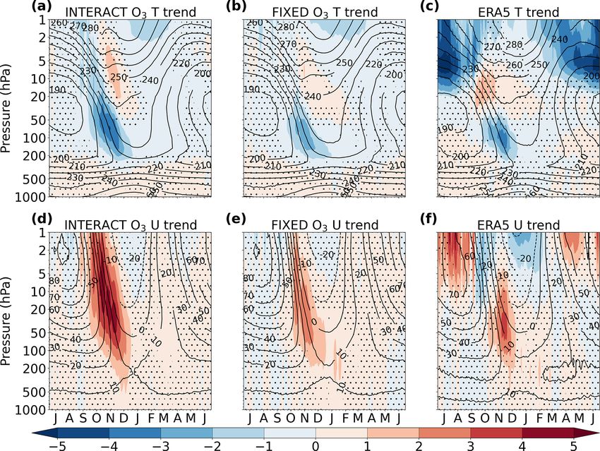
I. Ivanciu et al.: Effects of CMIP6 O3 on SH atmospheric circulation response to O3 depletion                                           5781

Table 1. Overview of the FOCI ensembles used in this study. Each ensemble consists of three simulations that vary in their initial conditions.

                   Ensemble           Ozone chemistry       GHGs                   ODSs                   Analysis period
                   FIXED O3           prescribed CMIP6      historical CMIP6       historical CMIP6       1958–2002
                   INTERACT O3        interactive           historical CMIP6       historical CMIP6       1958–2002
                   REF                interactive           historical CMIP6       historical CMIP6       1978–2002
                   NoODS              interactive           historical CMIP6       fixed at 1960s level   1978–2002
                   NoGHG              interactive           fixed at 1960s level   historical CMIP6       1978–2002

in GHGs past this date. This experimental design allows us               2.2    Observational data
to quantify the impact of the formation of the ozone hole by
taking the difference between REF and NoODS and that of                  The Integrated Global Radiosonde Archive (IGRA) version 2
climate change by taking the difference between REF and                  (Durre et al., 2006) temperature was used in order to com-
NoGHG. All of these sensitivity simulations use the FOCI                 pare the temperature trends simulated by the FOCI ensem-
configuration that includes interactive chemistry such that              bles with observational estimates. Data from 11 Antarctic
the chemical–radiative–dynamical feedbacks are captured                  stations located south of 65◦ S offering sufficient coverage
and the ozone field is consistent with the simulated dynam-              for the period 1958–2002 were averaged for each day and
ics. Additionally, the high-resolution ocean nest INALT10X               pressure level up to 30 hPa. As only the South Pole station is
(Schwarzkopf et al., 2019) was used for these simulations.               located south of 80◦ S, a trend computed for the entire polar
Therefore, the REF ensemble differs from the INTERACT                    cap is biased towards the lower latitudes, and only the trend
O3 ensemble discussed below. The INALT10X nest enhances                  derived from the spatial average over the 65–80◦ S latitude
the ocean resolution to 1/10◦ over the South Atlantic Ocean,             band is shown in Fig. 10. The full polar cap IGRA tempera-
the western part of the Indian Ocean, and the correspond-                ture trend is sown in the Supplement in Fig. S5. In addition,
ing Southern Ocean sectors, resolving the mesoscale eddies               the temperature and wind from the ERA5 reanalysis (Hers-
found in these regions and allowing us to assess, in a follow-           bach et al., 2020) were used to further verify the trends ob-
up study, the influence of climate change and ozone depletion            tained from our model.
on the ocean circulation around the tip of South Africa.
   In order to analyze the differences between simulations               2.3    Methodology
with interactive ozone chemistry and simulations with pre-
scribed CMIP6 ozone, two further ensembles were per-                     We used the transformed Eulerian mean framework (An-
formed, each consisting of three simulations differing only              drews et al., 1987) to calculate the residual circulation and
in their initial conditions. For the INTERACT O3 ensemble,               its forcing. According to the downward control principle of
FOCI was run in the configuration with interactive chemistry             Haynes et al. (1991), the residual downward velocity w∗ at
such that the chemical reactions that are necessary to repre-            a certain level is driven by the wave dissipation at the lev-
sent stratospheric chemical processes were included. There-              els above. The divergence of the Eliassen–Palm (EP) flux,
fore, the feedbacks between the stratospheric ozone, temper-             (a cos φ)−1 ∇ · F , gives a measure of the dissipation of re-
ature, and dynamics occur in INTERACT O3 and the simu-                   solved waves, where
lated ozone field is consistent with the dynamics. A compar-                          1 ∂(Fφ cos φ) ∂Fp
ison of the ozone field simulated in INTERACT O3 with ob-                ∇ ·F =                    +    .                                 (1)
                                                                                   a cos φ ∂φ        ∂p
servations can be found in the work of Matthes et al. (2020).
For the FIXED O3 ensemble, the ozone field recommended                   The components of the EP flux are given by
for CMIP6 (Hegglin et al., 2016) was prescribed. The CMIP6
ozone field was generated by two CCMs and includes so-                   Fφ = −a cos φv 0 u0 ,                                            (2)
lar variations from the SOLARIS-HEPPA project (Matthes
et al., 2017). It is a monthly mean three-dimensional field and                           v0θ 0
                                                                         Fp = f a cos φ           .                                       (3)
therefore includes zonal asymmetries in ozone. The monthly                                 θp
mean values were linearly interpolated and prescribed at each
model time step. The comparison of the INTERACT O3 and                   The notation is the same as in Andrews et al. (1987): the
FIXED O3 ensembles sheds light on the impact of prescrib-                overbars denote the zonal mean and the primes denote de-
ing the CMIP6 chemistry on the climate simulated by the                  partures from the zonal mean, a is the radius of the Earth, φ
coupled climate model FOCI.                                              is the latitude, u and v are the zonal and meridional veloc-
                                                                         ity components, respectively, f is the Coriolis parameter, θ
                                                                         is the potential temperature, and θp is the partial derivative
                                                                         of θ with respect to pressure. The residual vertical velocity

https://doi.org/10.5194/acp-21-5777-2021                                                    Atmos. Chem. Phys., 21, 5777–5806, 2021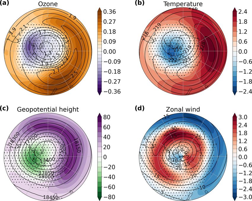
5782                         I. Ivanciu et al.: Effects of CMIP6 O3 on SH atmospheric circulation response to O3 depletion

was calculated from the streamfunction, as in McLandress           applying a Gaussian filter with a full width at half-maximum
and Shepherd (2009):                                               of 42 d over a 181 d window. An exponential function was
                                                                   then fitted to the smoothed ACF up to a lag of 50 d using the
         gH ∂9                                                     least squares method, and the SAM timescale was obtained
w∗ =               ,                                        (4)
       pa cos φ ∂φ                                                 by taking the lag at which the exponential function drops to
where the streamfunction is given by                               1/e.
                                                                      Linear trends were calculated over the 1958–2002 period
              Z0                                                   for the analyzed fields at each level and location, and the
     cos φ                                                         significance of the trends was assessed based on a Mann–
9 =−               v ∗ (φ, p)dp,                            (5)
       g                                                           Kendall test. Where differences between simulations are
               p
                                                                   shown, a two-sided t test was used to test for significance.
and the meridional residual velocity is given by                   The significance is always given at the 95 % confidence in-
                                                                   terval. The differences between the REF and the NoODS or
            ∂  v0θ 0                                             NoGHG ensembles were computed over the 1978–2002 pe-
v∗ = v −               ,                                    (6)    riod, as this is the period characterized by the strongest ozone
           ∂p θp
                                                                   depletion.
with g being the gravitational acceleration and H the scale
height taken as 7000 m. The shortwave (SW) and longwave
(LW) heating rates are part of the standard FOCI output, and       3   Impacts of ozone depletion and climate change on
the total radiative heating rate was obtained by taking the            Southern Hemisphere dynamics
sum of the two. The dynamical heating rate was calculated
as the difference between the temperature tendency at daily        The radiative effects of increasing GHG concentrations lead
resolution and the total radiative heating rate.                   to cooling of the stratosphere and warming of the tropo-
    The SAM was computed as the first empirical orthog-            sphere, enhancing the meridional temperature gradient at the
onal function (EOF) of the daily zonal mean geopotential           tropopause levels in a similar manner to ozone depletion.
height anomalies at each pressure level following the method       While some older studies argued that rising levels of GHGs
outlined in Gerber et al. (2010). To obtain the geopoten-          are the driver of the historical dynamical changes in the SH
tial height anomalies, the weighted global mean geopoten-          (Fyfe et al., 1999; Kushner et al., 2001; Marshall et al., 2004),
tial height was first subtracted for each day and at each level    at present the general consensus is that the formation of the
and latitude. A slowly varying climatology was then removed        Antarctic ozone hole is the main cause of these dynamical
to ensure that the resulting SAM index does not exhibit any        changes in austral spring and summer and that increasing
long-term trend driven by external climate forcing such that       GHGs played only a secondary role (Arblaster and Meehl,
it only reflects internal variability. The slowly varying clima-   2006; McLandress et al., 2011; Polvani et al., 2011; Kee-
tology was obtained by applying a 60 d low-pass filter to the      ble et al., 2014; Previdi and Polvani, 2014; World Meteoro-
geopotential height anomalies from the global mean. Then,          logical Organization, 2018). In this section, we separate the
time series were created for each day of the year and at each      effects of ozone depletion from those of increasing GHGs
location from the filtered anomalies, and each time series was     in FOCI, and we verify the ability of the model to correctly
smoothed using a 30-year low-pass filter. The smoothed time        simulate the dynamical response to ozone loss.
series were subtracted from the anomalies with respect to             Figure 1 shows the reduction in ozone above the Antarctic
the global mean for each respective day and location. The          polar cap caused by ODSs (panel a) together with the accom-
anomalies thus obtained were multiplied by the square root         panying changes in the SW heating rate (panel b). There is a
of the cosine of latitude in order to account for the conver-      strong decrease in the ozone volume mixing ratio in the lower
gence of the meridians towards the poles (North et al., 1982),     stratosphere in austral spring, peaking in October, in agree-
and only the anomalies for the SH were retained. The first         ment with previous studies (Perlwitz et al., 2008; Son et al.,
EOF of these anomalies was calculated at each pressure level,      2010; Polvani et al., 2011; Eyring et al., 2013). This leads to
and the expansion coefficients (principle component time se-       a significant radiative cooling due to decreased absorption of
ries) were obtained by projecting the anomalies onto the first     SW radiation (Fig. 1b). An even stronger SW cooling can be
EOF pattern. The expansion coefficients give the SAM index,        seen above 5 hPa between September and April, in line with
normalized to have zero mean and unit variance.                    the results of Langematz et al. (2003), who found a reduction
    The SAM e-folding timescale was computed for each day          of the SW heating rate in the upper stratosphere in response
of the year at each pressure level using the method of Simp-       to decreasing ozone concentrations. A significant SW warm-
son et al. (2011). The autocorrelation function (ACF) was          ing appears in December and January between 50 and 10 hPa,
obtained by correlating the time series for a particular day of    related to an increased ozone mixing ratio. As will be shown
the year with the time series for the days lagging and leading     later in this section, these latter changes are attributed to a
it. The ACF was smoothed at each lag and pressure level by         dynamical response to the spring ozone loss.

Atmos. Chem. Phys., 21, 5777–5806, 2021                                              https://doi.org/10.5194/acp-21-5777-2021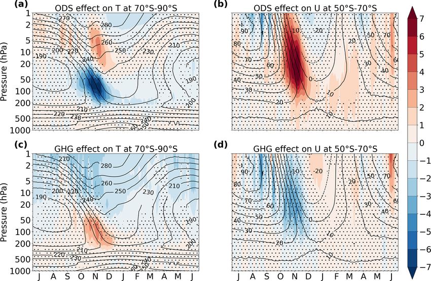
I. Ivanciu et al.: Effects of CMIP6 O3 on SH atmospheric circulation response to O3 depletion                                       5783

Figure 1. Seasonal cycle of the difference between REF and NoODS (a, b) and between REF and NoGHG (c, d) in the ozone volume mixing
ratio (a, c; ppmv) and the SW heating rate (b, d; K d−1 ) averaged over the polar cap (70–90◦ S) for the period 1978–2002. Stippling masks
values that are not significant at the 95 % confidence interval. The letter corresponding to each month marks the middle of that month.

   Figure 1c shows the ozone changes caused by increas-                significant enhancement of the downwelling over the polar
ing GHGs. There are two regions of statistically significant           cap between 50 and 200 hPa in the second half of October,
ozone increase: the upper stratosphere in austral spring and           which is associated with increased wave forcing between 20
summer and the region of the ozone hole. The SW heat-                  and 100 hPa (not shown). This suggests that changes in dy-
ing rate (Fig. 1d) exhibits warming in response to increased           namics are responsible for transporting more ozone into the
GHGs in the same two regions. As the direct effect of GHGs             polar lower stratosphere, in agreement with previous stud-
on the SW heating rate is small (Langematz et al., 2003), this         ies that linked a GHG-induced acceleration of the BDC to a
warming is likely caused by the higher ozone levels arising in         decrease in lower-stratospheric ozone in the tropics and an
response to the GHG increase, and not directly by the GHGs             increase at high latitudes (Dietmüller et al., 2014; Nowack
themselves. Higher levels of GHGs lead to increased emis-              et al., 2015; Chiodo et al., 2018). As a result, the strato-
sions of LW radiation (not shown) and have a net cooling               spheric ozone depletion is stronger in the absence of in-
effect in the stratosphere. In the upper stratosphere, lower           creased GHGs (NoGHG experiments) than in their presence
temperatures slow down ozone depletion (Haigh and Pyle,                (REF experiments). The ozone increase related to GHGs of
1982; Jonsson et al., 2004; Stolarski et al., 2010; Chiodo             about 0.2 ppmv, however, is small compared to the ozone
et al., 2018), explaining the simulated increase in ozone. The         loss due to ODSs, which exceeds 1.4 ppmv in the region of
ozone increase in the lower stratosphere is more surprising.           strongest depletion.
Here, colder conditions facilitate the formation of PSCs and              The polar cap temperature response to ozone depletion
are therefore expected to enhance ozone loss. Solomon et al.           (Fig. 2a) is closely related to the changes in the SW heat-
(2015) showed that a cooling of 2 K results in 30 DU more              ing rate shown in Fig. 1b. A statistically significant cooling
total column ozone loss over Antarctica. Therefore, it does            occurs in the lower stratosphere in austral spring and in the
not seem likely that the elevated ozone levels are caused by           upper stratosphere in summer. Additionally, there is a warm-
the radiative effects of GHGs. Instead, we find a small but            ing above the ozone hole in late spring. It should be noted

https://doi.org/10.5194/acp-21-5777-2021                                                 Atmos. Chem. Phys., 21, 5777–5806, 2021
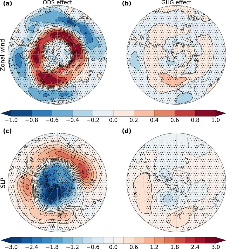
5784                         I. Ivanciu et al.: Effects of CMIP6 O3 on SH atmospheric circulation response to O3 depletion

Figure 2. Seasonal cycle of the difference between REF and NoODS (a, b) and between REF and NoGHG (c, d) in the polar cap (70–90◦ S)
temperature (a, c; K) and in the midlatitude (50–70◦ S) zonal wind (b, d; m s−1 ) for the period 1978–2002 (color shading). Stippling masks
values that are not significant at the 95 % confidence interval. Contours show the corresponding climatological temperature and zonal wind
from REF. The letter corresponding to each month marks the middle of that month.

that the maximum temperature increase above the ozone hole              strengthen on their poleward side and weaken on their equa-
occurs about 1 month earlier than the maximum shortwave                 torward side, shifting poleward. This shift is accompanied
warming, hinting at the fact that it is not a direct radiative          by changes in sea level pressure (SLP). The pressure over
effect of the increase in ozone. The temperature decreases              Antarctica drops significantly and the midlatitude SLP in-
are a direct response to ozone depletion. The spring cooling            creases in response to ozone depletion (Fig. 3c), signaling
in the lower stratosphere represents the well-known signature           a change towards the positive phase of the SAM. All these
of the ozone hole. In contrast to the impact of the ozone hole,         changes in the SH dynamics simulated in FOCI in response
there is no significant cooling in the polar lower stratosphere         to ozone depletion, both in the stratosphere and in the tro-
due to increased GHGs (Fig. 2c). The cooling resulting from             posphere, are in good agreement with the results of previous
enhanced LW emissions is confined to the upper levels of the            studies that isolated the impacts of ozone loss from those of
stratosphere. The lower stratosphere warms in November in               the increase in GHGs (Arblaster and Meehl, 2006; McLan-
response to GHGs. At these levels the SW warming (Fig. 1d)              dress et al., 2010, 2011; Polvani et al., 2011; Keeble et al.,
due to the elevated ozone concentrations dominates the LW               2014), as well as with the trends from observations and the
cooling (not shown) due to GHGs, resulting in a net radiative           ERA5 reanalysis presented in Sect. 4. This demonstrates that
warming.                                                                FOCI is able to capture the effects of ozone depletion and
   The zonal wind changes associated with ozone depletion               is therefore suited to studying how prescribing the CMIP6
(Fig. 2b) and increasing GHGs (Fig. 2d) obey the thermal                ozone affects the simulated climate response to ozone loss.
wind balance. The polar night jet accelerates from October                 The response of the stratospheric westerlies to higher
onwards as a consequence of the enhanced meridional tem-                GHG concentrations is markedly different from that to ozone
perature gradient caused by ozone loss. The maximum accel-              depletion (Fig. 2b, d). Driven by the warming over the polar
eration occurs between November and December (Fig. 2b),                 cap, the polar night jet weakens in November south of 60◦ S
concomitant with the strongest cooling (Fig. 2a). This west-            (Fig. S1 in the Supplement). This change is much weaker
erly acceleration propagates downwards to the tropospheric              compared to that resulting from ozone loss and is confined
eddy-driven jet and reaches the surface in November and De-             to the stratosphere. While GHGs do not cause an acceler-
cember. Figure 3a shows the ozone-induced change in the                 ation of the polar night jet in FOCI, there is a significant
surface zonal wind for these months. The surface westerlies             positive change in the zonal wind strength centered around

Atmos. Chem. Phys., 21, 5777–5806, 2021                                                    https://doi.org/10.5194/acp-21-5777-2021
I. Ivanciu et al.: Effects of CMIP6 O3 on SH atmospheric circulation response to O3 depletion                                  5785

Figure 3. Polar stereographic maps of the November–December difference between REF and NoODS (a, c) and the annual mean difference
between REF and NoGHG (b, d) in the surface zonal wind (a, b; m s−1 ) and in sea level pressure (c, d; hPa) for the period 1978–2002.
Stippling masks values that are not significant at the 95 % confidence interval.

30◦ S, extending from the top of the eddy-driven jet into the        this increase is less than a quarter of that due to ozone loss
middle stratosphere (Fig. S1). This westerly change implies          and there is no significant SLP decrease over the polar cap.
a strengthening of the upper flank of the tropospheric jet,             Our sensitivity experiments confirm that the changes in the
in agreement with the findings of McLandress et al. (2010).          SH polar night jet (Fig. 2b, d) and eddy-driven jet (Fig. 3a,
Figure 3b shows a map of the annual mean GHG-induced                 b) during the later part of the twentieth century were mainly
changes in the surface zonal winds. We show the annual               driven by ozone depletion. Increasing GHGs have played
mean change due to GHGs and not the November–December                only a minor role, acting to enhance the effect of the ozone
change as for the case of ozone depletion because, unlike the        hole in the troposphere and to partially counteract the impact
effects of ozone loss, the effects of increasing GHGs do not         of ozone loss on the polar night jet. In addition, we found
exhibit any seasonality. Although the GHG-induced pattern            that the upper stratosphere has cooled significantly and the
of zonal wind change is similar to that caused by ozone de-          troposphere has warmed significantly in response to increas-
pletion, the changes are much weaker and mostly insignifi-           ing concentrations of GHGs.
cant. This indicates that the magnitude of GHG increase was             Having distinguished the contributions of ozone loss and
not large enough to induce a strong strengthening or pole-           rising GHG levels to the changes in the westerly winds, we
ward shift of the surface westerly winds. The SLP response           now turn our attention to the impacts of ozone depletion
to increasing GHGs exhibits a significant increase in the mid-       on the BDC. Figure 4 shows the November ozone-induced
latitudes over the South Pacific Ocean, but the magnitude of         changes in the residual circulation, which is commonly used
                                                                     as a proxy for the BDC. The residual circulation is primarily

https://doi.org/10.5194/acp-21-5777-2021                                              Atmos. Chem. Phys., 21, 5777–5806, 2021
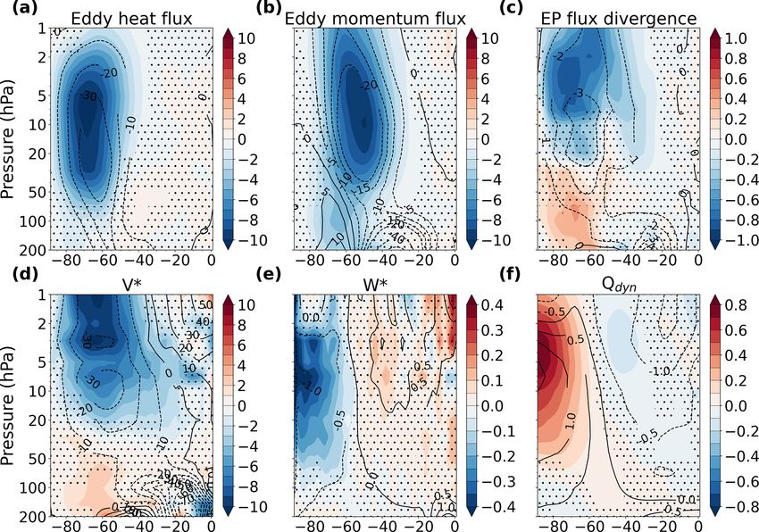
5786                          I. Ivanciu et al.: Effects of CMIP6 O3 on SH atmospheric circulation response to O3 depletion

Figure 4. November latitude–height difference between REF and NoODS in the eddy heat flux (a; K m s−1 ), the eddy momentum flux (b;
m2 s−2 ), the divergence of the EP flux (c; m s−1 d−1 ), the meridional residual velocity (d; cm s−1 ), the vertical residual velocity (e; mm s−1 ),
and the dynamical heating rate (f; K d−1 ) for the period 1978–2002 (color shading). Contours in each panel show the corresponding clima-
tology from REF. Stippling masks values that are not significant at the 95 % confidence interval.

forced by the dissipation of vertically propagating planetary               to propagate deeper into the stratosphere is related to the
waves from the troposphere. Therefore, we also present in                   strengthening of the polar night jet in response to ozone de-
Fig. 4 the changes in eddy heat and momentum fluxes, which                  pletion. Enhanced westerly velocities in November lead to
reveal the direction of wave propagation, and the changes                   a delay in the breakdown of the polar vortex (e.g., Waugh
in the divergence of the EP flux, which measures the wave                   et al., 1999; Langematz et al., 2003) and sustain wave activ-
forcing. The EP flux divergence (Fig. 4c) is characterized                  ity. McLandress et al. (2010) showed that, as a result of ozone
by a significant negative change above 10 hPa (stronger con-                depletion, (1) the height of the transition between westerly
vergence) and a significant positive change (weaker conver-                 and easterly velocities has increased, implying that waves
gence) in the lower stratosphere below 50 hPa. This implies                 can propagate higher at the end of spring, and (2) the date
a reduction of wave dissipation in the lower stratosphere and               of this transition has been delayed by 10 to 15 d, implying
an increase above, suggesting that atmospheric waves prop-                  that the period during which waves can penetrate into the
agating from the troposphere reach higher into the strato-                  stratosphere has been prolonged. As a result, the wave drag
sphere. This is confirmed by the strengthening of the eddy                  due to the dissipation of resolved waves increased in the up-
heat flux above 50 hPa (Fig. 4a). The eddy heat flux is equiv-              per stratosphere and decreased in the lower stratosphere in
alent to the vertical component of the EP flux and gives a                  November (Fig. 4c), while it increased in the middle strato-
measure of the vertical propagation of resolved waves. This                 sphere in December (Fig. S2), driving similar changes in
strengthening entails increased wave propagation in the mid-                the residual circulation. In November, the residual merid-
dle and upper stratosphere. Similarly, the eddy momentum                    ional velocity (Fig. 4d) shows a significant poleward inten-
flux exhibits a negative change, implying increased equator-                sification above 20 hPa and a significant weakening below
ward wave propagation (Fig. 4b). The ability of the waves                   50 hPa, in good agreement with the changes in the EP flux

Atmos. Chem. Phys., 21, 5777–5806, 2021                                                         https://doi.org/10.5194/acp-21-5777-2021
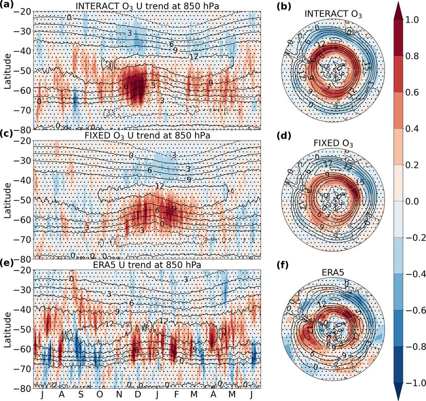
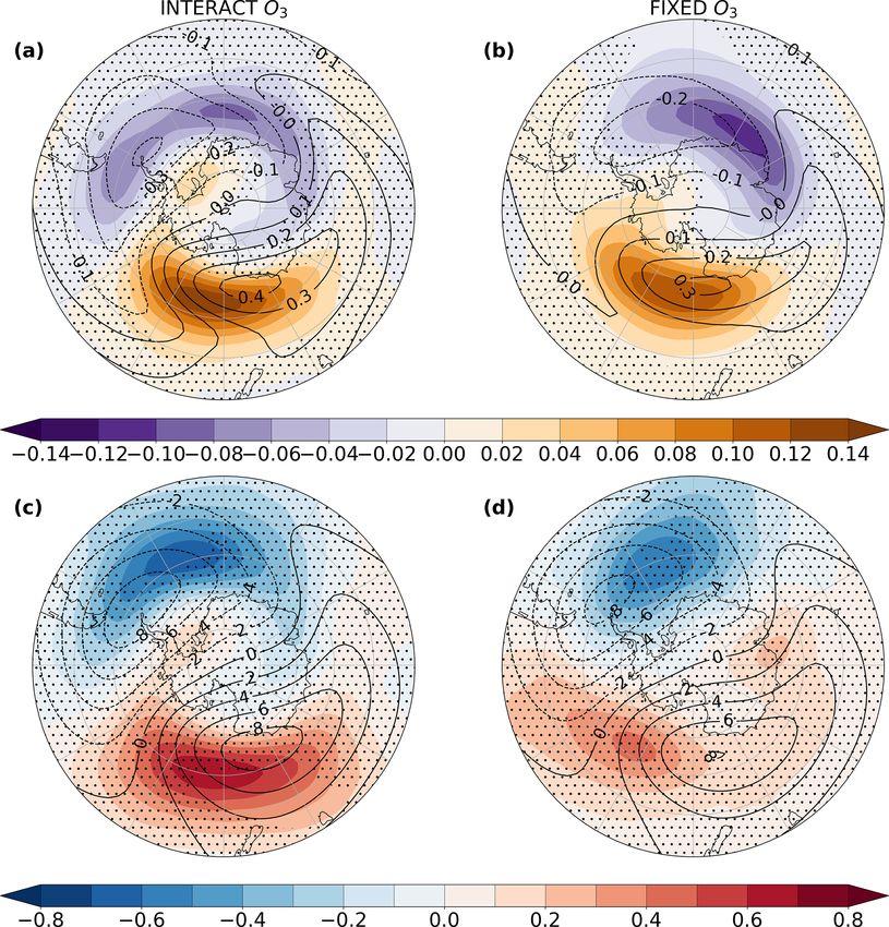
I. Ivanciu et al.: Effects of CMIP6 O3 on SH atmospheric circulation response to O3 depletion                               5787

divergence. The downwelling over the polar cap is enhanced        in the SH due to increasing GHGs. Therefore, we conclude
above 50 hPa (Fig. 4e). Associated with this intensification is   that the historical changes in the SH residual circulation over
a large dynamical warming (Fig. 4f) that increases the tem-       the period of ozone depletion are a consequence of the for-
perature above the ozone hole, as shown in Fig. 2a, consistent    mation of the ozone hole, in line with the findings of Keeble
with the results of Mahlman et al. (1994), Li et al. (2008),      et al. (2014), Oberländer-Hayn et al. (2015), Polvani et al.
Stolarski et al. (2010), Keeble et al. (2014), and Ivy et al.     (2018), Li et al. (2018), Abalos et al. (2019), and the most
(2016). At the same time, the strengthening of the residual       recent Scientific Assessment of Ozone Depletion (World Me-
circulation transports more ozone to the polar regions, lead-     teorological Organization, 2018). Consistent with these stud-
ing to the increase in ozone seen in December between 50          ies, FOCI simulates a strengthening of the SH residual cir-
and 10 hPa in Fig. 1a. The residual vertical velocity in the      culation in response to enhanced wave forcing at the end of
lower stratosphere is expected to weaken in response to the       the spring and the beginning of summer. At the same time, a
decreased wave drag seen in Fig. 4c below 50 hPa. Such a          weakening of the spring lower stratosphere residual circula-
weakening is simulated in FOCI at 200 hPa (Fig. 4e), accom-       tion is simulated, as found by the few studies that investigated
panied by a decrease in dynamical heating (Fig. 4f). How-         springtime changes in the BDC (Li et al., 2008; McLandress
ever, the lower-stratospheric change in downwelling is not        et al., 2010; Lubis et al., 2016). The good agreement with
significant at the 95 % confidence interval, and the change in    previous studies demonstrates that the interactive chemistry
the dynamical heating is only partly significant. The decrease    configuration of FOCI adequately simulates the impact of
in austral spring lower stratosphere downwelling was previ-       ozone depletion on the residual circulation.
ously reported by Li et al. (2008), McLandress et al. (2010),
and Lubis et al. (2016), while the decrease in dynamical heat-
ing was shown by Keeley et al. (2007), Orr et al. (2013), and     4     Effects of prescribing the CMIP6 ozone field
Lubis et al. (2016). Consistent with our results, McLandress
et al. (2010) also attributed their weaker downwelling to re-     We aim to understand how prescribing the ozone field recom-
duced wave drag in the austral spring. We note that Fig. 4        mended for CMIP6 affects the SH atmospheric circulation
displays changes averaged for the entire month of November.       response to ozone depletion. To this end, we compare an en-
However, the analysis of Orr et al. (2012, 2013) using 15 d       semble of simulations using prescribed CMIP6 ozone with an
averages showed that, at this time of the year, changes in the    ensemble of simulations that use fully interactive chemistry.
lower stratosphere wave driving and dynamical heating due         The use of an ozone field that differs from that internally
to ozone depletion occur over a shorter time. Therefore, it is    simulated by the model and that is not consistent with the
likely that our November averaging is applied over periods        model dynamics, the lack of chemical–radiative–dynamical
exhibiting changes of different sign, consequently diminish-      feedbacks, and the temporal interpolation from the monthly
ing the magnitude of the change and rendering it insignifi-       prescribed values to the model time step can all lead to dif-
cant. At the same time, the large internal variability in FOCI    ferences between the two ensembles. With a view on these
makes it hard to discern this change using fields with higher     deficiencies, we begin by analyzing the differences in the
temporal resolution, and more ensemble members would be           mean state in Sect. 4.1, and we then compare the simulated
needed to clearly detect the weakening in downwelling.            SH variability in Sect. 4.2 and the persistence of the SAM in
   The temporal evolution of the ozone-driven changes in          Sect. 4.3.
wave forcing and, as a result, in the residual circulation can
be seen by comparing Fig. 4 with Fig. S2, which shows the         4.1    Effects on the mean state
same quantities but for December. It is clear that there is a
downward propagation of the changes in all quantities from        Figure 5 shows the difference between INTERACT O3 and
November to December. As the polar vortex breaks down             FIXED O3 in October average ozone and November average
at the upper levels, the zonal velocities remain westerly be-     temperature, geopotential height, and zonal wind at 70 hPa.
low 50 hPa (contours in Fig. 2b) and are still able to sup-       The CMIP6 ozone field was used for FIXED O3 . FOCI sim-
port the remnant wave propagation. Stronger westerlies in         ulates significantly lower ozone levels above the Antarc-
the lower stratosphere in December imply enhanced wave            tic Peninsula and the Bellingshausen Sea in October com-
dissipation. As a result, the downwelling is accelerated in the   pared to the CMIP6 ozone (Fig. 5a). As a consequence, the
lower stratosphere, driving dynamical warming there. These        November temperature (Fig. 5b) and the geopotential height
results are consistent with those of McLandress et al. (2010)     (Fig. 5c) are also lower in this region in INTERACT O3 com-
and explain the reason behind the change in the sign of the       pared to FIXED O3 . We note that the pattern of the tempera-
residual vertical velocity trends in the lower stratosphere be-   ture difference between INTERACT O3 and FIXED O3 is
tween spring and summer.                                          markedly different to the pattern reported by Crook et al.
   Our results clearly show that ozone depletion had a signif-    (2008) and Gillett et al. (2009), which arises due to zonal
icant influence on the SH BDC in austral spring and summer.       asymmetries in ozone. The CMIP6 ozone field prescribed in
FOCI simulates little significant residual circulation change     FIXED O3 includes ozone asymmetries, and their effects are

https://doi.org/10.5194/acp-21-5777-2021                                           Atmos. Chem. Phys., 21, 5777–5806, 2021
5788                        I. Ivanciu et al.: Effects of CMIP6 O3 on SH atmospheric circulation response to O3 depletion

Figure 5. Polar stereographic maps of the difference between INTERACT O3 and FIXED O3 in the October mean ozone (a; ppmv) and the
November mean temperature (b; K), geopotential height (c; m), and zonal wind (d; m s−1 ) at 70 hPa (color shading). The stippling masks
regions that are not significant at the 95 % confidence interval. The overlaying contours mark the 1958–2013 INTERACT O3 climatology of
each respective variable and month.

therefore captured in FIXED O3 . Despite this, spatial tem-           perature outside the polar vortex in INTERACT O3 enhances
perature and geopotential height differences still remain be-         the meridional pressure gradient between the polar low and
tween simulations with prescribed ozone asymmetries and               the midlatitude high. In the Pacific sector, the meridional
simulations with fully interactive ozone chemistry because            pressure gradient is stronger in INTERACT O3 due to the
the prescribed ozone field differs from the simulated one and         lower temperature above West Antarctica and the Belling-
is not consistent with the simulated dynamics.                        shausen Sea. As a result, the November polar night jet is cir-
   The differences between the FOCI and CMIP6 ozone                   cumpolarly stronger in INTERACT O3 compared to FIXED
fields are not confined just to the ozone hole itself. Outside        O3 (Fig. 5d).
the polar vortex, INTERACT O3 exhibits significantly higher              To better understand the cause of the lower ozone levels
ozone levels at all longitudes. The difference in ozone max-          above the Antarctic Peninsula and the Bellingshausen Sea in
imizes in the eastern hemisphere, as the polar vortex, and            INTERACT O3 , Fig. 6c shows the October average ozone
hence the ozone hole, is not centered over the pole but dis-          anomalies from the zonal mean in INTERACT O3 at 70 hPa
placed towards the Atlantic Ocean and South America (con-             and the difference to FIXED O3 . A zonal wavenumber one
tours in Fig. 5a). This significant positive difference was           pattern is clearly visible, with the ridge at the edge of Antarc-
found in the middle to high latitudes of both hemispheres and         tica towards New Zealand and the trough over the tip of the
in all seasons (not shown). We hypothesize that it is the result      Antarctic Peninsula. The ozone wave simulated in FOCI is
of a stronger BDC in FOCI compared to the models used to              consistent with that inferred from satellite observations by
generate the CMIP6 ozone field, leading to increased ozone            Lin et al. (2009) and Grytsai et al. (2007), from reanalyses by
transport from the tropics. Associated with the higher ozone          Crook et al. (2008), and with that simulated by Gillett et al.
levels, the November midlatitude temperature and geopoten-            (2009). This wave pattern confirms that the simulated ozone
tial height are also elevated in INTERACT O3 compared to              hole is not centered on the South Pole. While the CMIP6
FIXED O3 . In the Atlantic and Indian sectors, the higher tem-        ozone hole is also displaced from the pole, its location and

Atmos. Chem. Phys., 21, 5777–5806, 2021                                                 https://doi.org/10.5194/acp-21-5777-2021
I. Ivanciu et al.: Effects of CMIP6 O3 on SH atmospheric circulation response to O3 depletion 5789
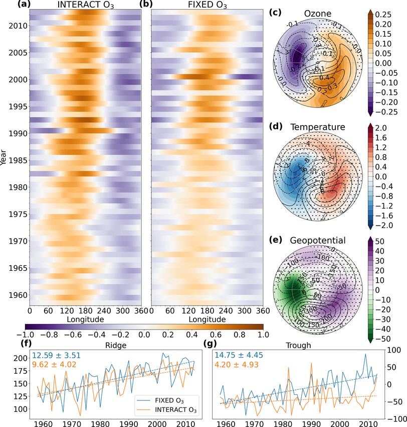
Figure 6. Hovmöller diagram of the October anomalies from the zonal mean ozone volume mixing ratio (ppmv) in INTERACT O3 (a) and
FIXED O3 (b) averaged over 60–70◦ S and maps of the October difference between INTERACT O3 and FIXED O3 in the anomalies from
the zonal mean ozone volume mixing ratio (c; ppmv), temperature (d; K), and geopotential height (e; m) at 70 hPa for the period 1958-2013
(color shading). The stippling in panels (c)–(e) masks regions that are not significant at the 95 % confidence interval. The overlaying contours
mark the INTERACT O3 1958–2013 average anomalies from the zonal mean for each respective variable. Time series of the longitude of the
ozone ridge maximum (f) and of the ozone trough minimum (g) for INTERACT O3 (solid orange lines) and FIXED O3 (solid blue lines),
together with their corresponding trends for the period 1958–2013 (dashed lines). The values of the trends are in degrees of longitude per
decade, and their 95 % confidence interval according to a two-tailed t test is given in the upper left corner of each panel.
extent are not the same as those simulated by FOCI (compare Figure 6a and b show the time evolution of the ozone wave
contours in Fig. 7a and d). The difference shown in Fig. 6c re- averaged between 60 and 70◦ S for the month of October for
veals that, on the one hand, the trough of the wave is shifted INTERACT O3 and FIXED O3 , respectively. Despite consid-
towards South America and reaches deeper into the Pacific erable interannual variability, the westward shift of the wave
sector in INTERACT O3 . On the other hand, the amplitude in INTERACT O3 compared to that in FIXED O3 is clearly
of the wave is significantly greater in INTERACT O3 (also discernable. This can be attributed to different evolutions of
compare contours in Fig. 8a and b). Figure 6c thus demon- the wave trough in the two ensembles. Figure 6f and g show
strates that the prescribed CMIP6 ozone field is not spatially the time series of the longitudes at which the ozone maxi-
consistent with the polar vortex simulated in FOCI. mum occurs within the ridge of the wave and at which the
ozone minimum occurs within the trough of the wave, re-
https://doi.org/10.5194/acp-21-5777-2021 Atmos. Chem. Phys., 21, 5777–5806, 2021You can also read