Oxygen budget of the north-western Mediterranean deep-convection region
←
→
Page content transcription
If your browser does not render page correctly, please read the page content below
Biogeosciences, 18, 937–960, 2021
https://doi.org/10.5194/bg-18-937-2021
© Author(s) 2021. This work is distributed under
the Creative Commons Attribution 4.0 License.

Oxygen budget of the north-western Mediterranean deep-
convection region
Caroline Ulses1,2 , Claude Estournel1 , Marine Fourrier3 , Laurent Coppola3 , Fayçal Kessouri2,4 , Dominique Lefèvre5 ,
and Patrick Marsaleix1
1 Laboratoire d’Etudes en Géophysique et Océanographie Spatiales (LEGOS), Université de Toulouse,
CNES, CNRS, IRD, UPS, Toulouse, France
2 Laboratoire d’Aérologie (LA), Université de Toulouse, CNRS, UPS, Toulouse, France
3 Sorbonne Université, CNRS, Laboratoire d’Océanographie de Villefranche (LOV), 06230 Villefranche-sur-Mer, France
4 Southern California Coastal Water Research Project, Costa Mesa, CA, USA
5 Aix-Marseille Université, Mediterranean Institute of Oceanography (MIO), 13288 Marseille CEDEX 9, France

Correspondence: Caroline Ulses (caroline.ulses@legos.obs-mip.fr)

Received: 17 July 2020 – Discussion started: 12 August 2020
Revised: 13 November 2020 – Accepted: 26 November 2020 – Published: 10 February 2021

Abstract. The north-western Mediterranean deep convec-            in this region predicted by the end of the century in recent
tion plays a crucial role in the general circulation and bio-     projections may have important consequences on the over-
geochemical cycles of the Mediterranean Sea. The DEWEX            all uptake of atmospheric oxygen in the Mediterranean Sea
(DEnse Water EXperiment) project aimed to better un-              and on the oxygen exchanges with the Atlantic Ocean, which
derstand this role through an intensive observation plat-         appear necessary to better quantify in the context of the ex-
form combined with a modelling framework. We developed            pansion of low-oxygen zones.
a three-dimensional coupled physical and biogeochemical
model to estimate the cycling and budget of dissolved oxygen
in the entire north-western Mediterranean deep-convection
area over the period September 2012 to September 2013.            1   Introduction
After showing that the simulated dissolved oxygen concen-
trations are in a good agreement with the in situ data col-       Deep convection is a key process leading to a massive trans-
lected from research cruises and Argo floats, we analyse the      fer of oxygen from the atmosphere to the ocean interior
seasonal cycle of the air–sea oxygen exchanges, as well as        (Körtzinger et al., 2004, 2008b; Fröb et al., 2016; Wolf et
physical and biogeochemical oxygen fluxes, and we estimate        al., 2018). Its weakening in some regions (de Lavergne et
an annual oxygen budget. Our study indicates that the an-         al., 2014; Brodeau and Koenigk, 2016), induced by enhanced
nual air-to-sea fluxes in the deep-convection area amounted       stratification, is one of the primary factors, along with chang-
to 20 mol m−2 yr−1 . A total of 88 % of the annual uptake         ing ventilation at intermediate depths, slowdown of the over-
of atmospheric oxygen, i.e. 18 mol m−2 , occurred during the      turning circulation, warming-induced decrease in solubility
intense vertical mixing period. The model shows that an           modulated by salinity changes and changes in C : N utili-
amount of 27 mol m−2 of oxygen, injected at the sea sur-          sation ratios, that may explain the ongoing decline in the
face and produced through photosynthesis, was transferred         open-ocean oxygen inventory, or deoxygenation, observed
under the euphotic layer, mainly during deep convection.          and modelled since the middle of the 20th century (Bopp et
An amount of 20 mol m−2 of oxygen was then gradually ex-          al., 2002; Keeling and Garcia, 2002; Plattner et al., 2002;
ported in the aphotic layers to the south and west of the west-   Joos et al., 2003; Keeling et al., 2010; Helm et al., 2011; An-
ern basin, notably, through the spreading of dense waters re-     drews et al., 2017; Ito et al., 2017; Schmidtko et al., 2017;
cently formed. The decline in the deep-convection intensity       Breitburg et al., 2018). The oxygen decline leads to an in-
                                                                  crease in the volume of hypoxic or even anoxic waters and

Published by Copernicus Publications on behalf of the European Geosciences Union.
938                             C. Ulses et al.: Oxygen budget of the north-western Mediterranean deep convection region

to the expansion of oxygen minimum zones (OMZs), which              (Tanhua et al., 2013). In the western Mediterranean open
substantially affect life and habitats of marine ecosystems         sea, the oxygen minimum layer (OML) is located in the
and have implications for biogeochemical cycles (Ingall et          LIW and shows a minimum oxygen concentration of 170–
al., 1994; Levin, 2003; Diaz and Rosenberg, 2008; Breit-            185 µmol kg−1 , above ≈ 70 % of the saturation levels (Tan-
burg et al., 2009; Naqvi et al., 2010; Stramma et al., 2010;        hua et al., 2013; Coppola et al., 2018). Thus the OML in
Scholz et al., 2014; Bristow et al., 2017). It is crucial to gain   this region is clearly less pronounced than the OMZs in the
understanding of the actual ventilation occurring in deep-          open oceans or deep basins of other seas, such as the adjacent
convection areas and to continue developing models to pre-          Black Sea, where hypoxic conditions (oxygen concentration
dict its future evolution under climate change.                     < 2 mL O2 L−1 or < 61 µmol O2 kg−1 ; Diaz and Rosenberg,
   The north-western (NW) Mediterranean Sea (Fig. 1a and            2008; Breitburg et al., 2018) are encountered. However the
b) is one of the few regions of the world where deep convec-        semi-enclosed Mediterranean Sea with a fast warming was
tion takes place (Schott et al., 1996). In autumn, during the       identified as one of the most vulnerable marine regions to cli-
preconditioning phase, a cyclonic gyre formed by the North-         mate change (Giorgi, 2006). Recently, regional ocean models
ern Current and the Balearic front leads to the doming of the       of the Mediterranean Sea converged to predict a weakening
isopycnals and the rising of high-salinity intermediate wa-         of NW deep-convection intensity under climate change sce-
ters, the Levantine Intermediate Waters (LIW), close to the         narios by the end of the 21st century (Soto-Navarro et al.,
surface. In winter, cold and dry northerly winds (Mistral, Tra-     2020). Yet, Coppola et al. (2018), by analysing the evolu-
montane) produce the cooling, evaporation and subsequent            tion of observed oxygen profiles in the Ligurian Sea over a
density increase in surface waters. The instability of the wa-      20 year period, suggested that hypoxic conditions may be
ter column induces convective mixing of surface waters with         reached in water masses at intermediate depths after a pe-
deeper waters, and, when the process is intense, in the forma-      riod of 25 years without deep-convection events (presuming
tion of new deep waters that spread into the western Mediter-       bacterial respiration remains the same).
ranean Sea, such as observed in 2004–2006 (Schroeder et al.,           One of the objectives of the DEWEX (DEnse Water EX-
2008a). The depth and horizontal extension of convection in         periment) project carried out in 2012/13 was to investigate
the NW region show strong interannual variability, driven by        the deep-convection process, the formation of north-western
both the variability of the winter buoyancy loss and the strat-     Mediterranean Deep Waters and the impact of deep convec-
ification magnitude prior to the convection period (Mertens         tion on biogeochemical fluxes (Conan et al., 2018). Three
and Schott, 1998; Béthoux et al., 2002; Houpert et al., 2016;       cruises and the deployment of autonomous platforms (glider,
Somot et al., 2016). The deepest convection takes place in          Argo floats) provided an unprecedented intensive observa-
the centre of the Gulf of Lion where the yearly maximum of          tion of this region before, during and after a deep-convection
the mixed-layer depth varies from a few hundred metres to           event and completed the observation effort during the strat-
2500 m when the bottom is reached (MEDOC Group, 1970).              ified period operated since 2010 in the framework of the
   At the Mediterranean basin scale, the deep convection oc-        MOOSE-GE (Mediterranean Ocean Observing System for
curring in the north-western region is one of the major pro-        the Environment-Grande Échelle) programme (Estournel et
cesses responsible for an enrichment of the euphotic layer          al., 2016b). The 2012/13 event was identified by observa-
with nutrients, compared to Atlantic influx as well as terres-      tional and modelling studies as one of the five most intense
trial and atmospheric inputs (Severin et al., 2014; Ulses et al.,   deep-convection events over the period 1980–2013 (Somot
2016; Kessouri et al., 2017). The replenishment of the sur-         et al., 2016; Herrmann et al., 2017; Coppola et al., 2018) due
face layer with nutrients during deep convection is followed        to extremely strong buoyancy loss (Somot et al., 2016). Re-
by an intense bloom in spring when vertical mixing weak-            garding the oxygen dynamics, DEWEX winter observations
ens (Bernadello et al., 2012; Lavigne et al., 2013; Auger et        showed a strong increase in the O2 inventory of the entire
al., 2014; Ulses et al., 2016; Kessouri et al., 2018). The for-     water column, which was concomitant to the deepening of
mation of deep waters is also at the origin of a huge venti-        the mixed layer and was attributed to a rapid intake of atmo-
lation of the western Mediterranean Sea (Minas and Bonin,           spheric dissolved oxygen (Coppola et al., 2017). However,
1988; Copin-Montégut and Bégovic, 2002; Schroeder et al.,           these observations remain limited in time and space. Up to
2008a; Schneider et al., 2014; Stöven and Tanhua, 2015;             date, no high-resolution modelling of the oxygen dynamics
Touratier et al., 2016; Coppola et al., 2017; 2018; Li and Tan-     in the NW deep-convection region that could complete the
hua, 2020). The study of Mavropoulou et al. (2020), based           monitoring effort and provide quantification for the whole
on in situ observations over the period 1960–2011, indicated        area has yet been proposed.
that its variability is one of the main drivers of the inter-          In this study, we take advantage of the DEWEX project to
annual variability of the dissolved oxygen (O2 ) concentra-         implement and constrain with in situ observations a 3D cou-
tion in the deep waters of the western Mediterranean Sea.           pled physical–biogeochemical model representing the dy-
The oxygenation induced by recurrent intermediate and deep          namics of dissolved oxygen and to gain understanding in the
convection together with a relatively low primary produc-           variability of the oxygen inventory in the whole NW Mediter-
tion make the Mediterranean Sea a well-oxygenated basin             ranean deep-convection area, for the period between Septem-

Biogeosciences, 18, 937–960, 2021                                                       https://doi.org/10.5194/bg-18-937-2021
C. Ulses et al.: Oxygen budget of the north-western Mediterranean deep convection region                                          939

Figure 1. Domain and bathymetry (m) of (a) the forcing coupled NEMO-Eco3MS Mediterranean model (red contour) and of (b) the coupled
SYMPHONIE-Eco3MS western sub-basin model. The blue contour in (a) indicates the limits of the western sub-basin model. The red
contoured area in (b) corresponds to the deep-convection area. (c) Scheme of the downscaling strategy from the Mediterranean Sea to the
western sub-basin.

ber 2012 and September 2013. In this framework, we investi-           is calculated using the bulk formulae described by Large
gate the seasonal cycle of the oxygen inventory and estimate          and Yeager (2004). This model was previously used in the
its annual budget, and we analyse and quantify the relative           Mediterranean Sea to simulate open-sea convection (Her-
contribution of air–sea exchanges, as well as of physical and         rmann et al., 2008; Estournel et al., 2016a; Ulses et al., 2016),
biogeochemical processes in the budget. The following doc-            shelf dense-water cascading (Estournel et al., 2005; Ulses et
ument is organised as follows: in Sect. 2, we describe the nu-        al., 2008b) and continental shelf circulation on the Gulf of
merical model, its implementation and the observations used           Lion shelf (Estournel et al., 2001; 2003; Ulses et al., 2008a).
for its assessment. In Sect. 3, we compare our model results
with in situ observations. In Sect. 4, we describe the seasonal       2.1.2   The biogeochemical model
cycle of atmospheric and physical conditions. In Sect. 5, we
examine the seasonal cycle of oxygen inventory and fluxes,            The biogeochemical model Eco3M-S is a multi-nutrient and
as well as the annual oxygen budget. We discuss our results           multi-plankton functional type model that simulates the dy-
in Sect. 6 and conclude in Sect. 7.                                   namics of the biogeochemical decoupled cycles of several
                                                                      biogenic elements (carbon, nitrogen, phosphorus, silicon)
                                                                      and of non-Redfieldian plankton groups (Ulses et al., 2016).
2     Material and methods                                            The model was previously used to study the biogeochemical
                                                                      processes on the Gulf of Lion shelf (Auger et al., 2011) and
2.1     The numerical model                                           in the NW Mediterranean deep-convection area (Herrmann
                                                                      et al., 2013, 2017; Auger et al., 2014; Ulses et al., 2016;
2.1.1    The hydrodynamic model                                       Kessouri et al., 2017, 2018). In this study, the model was ex-
                                                                      tended to describe the dynamics of dissolved oxygen in the
The SYMPHONIE model used in this study is a 3D primitive              ocean interior and the air–sea exchanges of oxygen. Here we
equation model, with a free surface and generalised sigma             only describe the rate of change of the new state variable, the
vertical coordinate, as described in Marsaleix et al. (2008).         dissolved oxygen concentration and the parameterisation of
The vertical diffusion is parameterised with a prognostic             the air–sea flux of oxygen, which were included in the model
equation for the turbulent kinetic energy and a diagnostic            version described in detail by Auger et al. (2011). The rate
equation for the mixing and dissipation lengths, following            of change of dissolved oxygen concentration due to biogeo-
Gaspar et al. (1990). Atmospheric forcing (turbulent fluxes)          chemistry in the water column is governed by the following

https://doi.org/10.5194/bg-18-937-2021                                                          Biogeosciences, 18, 937–960, 2021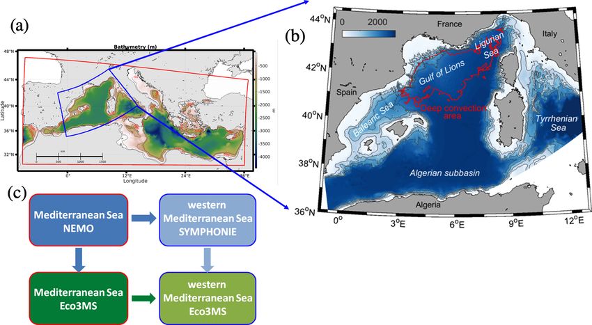
940                            C. Ulses et al.: Oxygen budget of the north-western Mediterranean deep convection region

equation:                                                          resolution (Bentsen et al., 1999). The mesh size ranges from
                                                                   0.8 km in the north to 1.4 km in the south. The grid has 40
       3                                                           vertical levels with closer spacing near the surface (15 levels
dDOx X
    =     GPPi − RespPhyi γC/DOx −                          (1)    in the first 100 m in the centre of the convection area charac-
 dt   i=1
                                                                   terised by depths of ≈ 2500 m). As explained in Estournel et
            3
            X                                                     al. (2016a), the size of the grid is not small enough to explic-
                  RespZooi + RespZooadd
                                    i     γC/DOx −
                                                                   itly represent convective plumes, which thus need to be pa-
            i=1
                                                                   rameterised. In our case, to prevent the development of static
         RespBac γC/DOx − Nitrif γNH4 /DOx ,                       instabilities at the surface resulting in noise at the scale of
                                                                   the mesh, the heat and water fluxes are distributed over the
where DOx is the dissolved oxygen concentration; GPPi
                                                                   whole mixed layer whose thickness is given by the depth at
and RespPhyi are gross primary production and respira-
                                                                   which the vertical density gradient becomes negative.
tion, respectively, for phytoplankton group i; RespZooi and
                                                                      The biogeochemical model is forced offline by daily out-
RespZooaddi   are basal respiration and additional respiration
                                                                   puts of the hydrodynamic model. The advection and diffu-
fluxes to maintain constant N : C and P : C internal ratios,
                                                                   sion of the biogeochemical variables were calculated using
respectively, for zooplankton group i; RespBac is bacterial
                                                                   the QUICKEST (QUICK with Estimated Streaming Terms)
respiration; and Nitrif is nitrification. γC/DOx and γNH4 /DOx ,
                                                                   scheme (Leonard, 1979) on the horizontal and with a centred
equal to 1 and 2, respectively, are the mole of DOx , used per
                                                                   scheme on the vertical.
mole of C in respiration and needed to oxidise 1 mol of am-
                                                                      A strategy of downscaling from the Mediterranean basin to
monium in nitrification as described in Grégoire et al. (2008).
                                                                   the western sub-basin scale was implemented in three stages
   The flux of dissolved oxygen at the air–sea interface,
                                                                   (Fig. 1a and c) as described by Kessouri et al (2017). In a first
DOx Flux, is computed from
                                                                   step, the SYMPHONIE hydrodynamic model was initialised
DOx Flux = Kw (DOx sat − DOx surf ) ,                       (2)    and forced at its lateral boundaries with daily analyses of the
                                                                   configuration PSY2V4R4, based on the NEMO ocean model
where DOx sat and DOx surf (mmol m−3 ) are the concentra-          at a resolution of 1/12◦ over the Atlantic and the Mediter-
tion of dissolved oxygen at saturation level and at the surface    ranean Sea by the Mercator Ocean International operational
of the ocean, respectively, and Kw (m s−1 ) is the gas trans-      system (Lellouche et al., 2013). Second, the biogeochemi-
fer velocity. The oxygen solubility (or dissolved oxygen at        cal model was forced at the Mediterranean basin scale by
saturation level) is determined using the equation of Garcia       the outputs of the same NEMO simulation. In a third step,
and Gordon (1992). The oxygen saturation anomaly (noted            the daily outputs of the two previous simulations were used
1O2 ) is defined as 1O2 = (DOx −DOx sat )/DOx sat ×100 %.          to initialise and force the Eco3M-S biogeochemical model
We computed here the gas transfer velocity using the param-        over the western Mediterranean Sea. This nesting protocol
eterisation of Wanninkhof and McGillis (1999) with a cu-           ensures the coherence of the physical and biogeochemical
bic dependency to the wind speed, following the study in the       fields at the open boundaries. The basin configuration of
convective Labrador Sea by Körtzinger et al. (2008b), who          the biogeochemical model was initialised in summer 2011,
found that this parameterisation was one of those that gave        with climatological fields of in situ nutrient concentrations
the best results and recommended a stronger-than-quadratic         from the oligotrophic period in the MEDAR/MEDATLAS
wind speed dependency for the high wind speed range. In            database (Manca et al., 2004) and according to oxygen ob-
addition, sensitivity analyses using eight various parameter-      servations from the Meteor M84/3 cruise carried out in April
isations of the gas transfer velocity were performed to esti-      2011 (Tanhua et al., 2013) and DYFAMED station observa-
mate uncertainties of air–sea exchanges and are discussed in       tions in August 2011 (Coppola et al., 2018). The regional
Sect. 6.1. For these sensitivity tests, we used quadratic (Wan-    biogeochemical simulation started in August 2012. Due to
ninkhof, 1992, 2014) and hybrid (Nightingale et al., 2000;         strong vertical diffusivities in the basin-scale model, we cor-
Wanninkhof et al., 2009) wind speed dependency parameter-          rected the initial oxygen concentration for the north-western
isations, as well as parameterisations including air–sea fluxes    region using DYFAMED observations carried out in the sum-
due to bubble formation (Woolf, 1997; Stanley et al., 2009;        mer of 2012 (Coppola et al., 2018) and for the south-western
Liang et al., 2013; Bushinsky and Emerson, 2018).                  region according to Meteor M84/3 observations.
                                                                      Meteorological parameters including downward radiative
2.1.3   Implementation                                             fluxes were taken from the ECMWF (European Centre for
                                                                   Medium-Range Weather Forecasts) operational forecasts at
The implementation of the hydrodynamic and biogeochemi-            1/8◦ horizontal resolution and 3 h temporal resolution based
cal simulations used in this study was described by Estournel      on daily analyses. River runoffs were considered based on
et al. (2016a) and Kessouri et al. (2017; 2018). The numeri-       realistic daily values for French rivers (data provided by
cal domain (Fig. 1a, b) covers most of the western Mediter-        Banque Hydro, http://www.hydro.eaufrance.fr/) and Ebro
ranean basin, using a curvilinear grid with variable horizontal    (data provided by SAIH Ebro, http://www.saihebro.com),

Biogeosciences, 18, 937–960, 2021                                                      https://doi.org/10.5194/bg-18-937-2021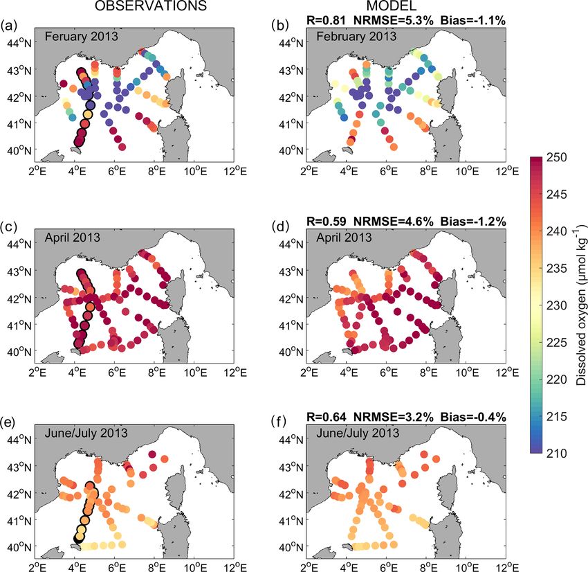
C. Ulses et al.: Oxygen budget of the north-western Mediterranean deep convection region                                      941

and mean annual values for the other rivers. At the Rhône          first one, DEWEX Leg1, was carried out during the active
River mouth, nitrate, ammonium, phosphate, silicate and dis-       phase of deep convection, in February 2013 (Testor, 2013),
solved organic carbon concentrations were prescribed us-           and the second one, DEWEX Leg2, was carried out during
ing in situ daily data (P. Raimbault, MISTRALS database).          the following spring bloom, in April 2013 (Conan, 2013).
These data, combined with those of Moutin et al. (1998) and        In addition, we use observations from the 2013 MOOSE-GE
Sempéré et al. (2000), were used to estimate dissolved or-         cruise, conducted during the stratified, oligotrophic season,
ganic phosphorus and nitrogen and particulate organic mat-         in June–July 2013 on board RV Tethys II (Testor et al., 2013).
ter concentrations as described in Auger et al. (2011). At the     The dissolved oxygen measurements were performed dur-
other river mouths, climatological values were prescribed ac-      ing the DEWEX (Leg1: 74 stations, Leg2: 99 stations) and
cording to Ludwig et al. (2010). Dissolved oxygen concen-          MOOSE-GE (74 stations) cruises, using a Sea-Bird SBE43
tration at the river mouths was set to values at saturation. The   sensor. The calibration and quality control of the measure-
deposition of organic and inorganic matter from the atmo-          ments were described by Coppola et al. (2017). The accu-
sphere was neglected in this study. Fluxes of inorganic nutri-     racy of the measurements was estimated at 2 % of oxygen
ents and oxygen at the sediment–sea interface were consid-         saturation, i.e. 4 µmol kg−1 . A Winkler analysis performed
ered by coupling the pelagic model with a simplified version       on board was used to adjust the SBE43 raw data, as specified
of the meta-model described by Soetaert et al. (2001). The         by the GO-SHIP programme (http://www.go-ship.org/).
parameters of the latter model were set following the mod-            We also compare our model results with high-frequency
elling study performed by Pastor et al. (2011) for the Gulf of     measurements of wind at 10 m and of ocean surface
Lion shelf.                                                        temperature, salinity (thermosalinograph and conductivity–
                                                                   temperature–depth (CTD)) and dissolved oxygen concentra-
2.1.4    Study area                                                tion (optode) at 3 m depth using the sea surface water contin-
                                                                   uous acquisition system (SACES) (Dugenne, 2017) during
For analyses and budget purposes, we defined the deep-             the two DEWEX cruises.
convection area as the area where the daily averaged
mixed-layer depth exceeded 1000 m at least once during
wintertime (red contoured area in Fig. 1b), according to           2.2.2    Argo floats
Kessouri et al. (2017, 2018). It covered an area of 61 720 km2
in 2013. The mixed-layer depth is defined as the depth where
                                                                   To evaluate the temporal evolution of the modelled oxy-
the potential density exceeds its value at 10 m depth by
                                                                   gen inventory, we use data of three Argo-O2 floats (floats
0.01 kg m−3 (Coppola et al., 2017). Heat fluxes and physical
                                                                   6901467, 6901470, 6901487) deployed in the NW Mediter-
and biogeochemical parameters and fluxes presented in
                                                                   ranean Sea during the preconditioning phase (late November
the following sections correspond to values averaged over
                                                                   2012) and the active phase (late January 2013) of dense wa-
all model grid points included in this area. The budget of
                                                                   ter formation and operational until the end of the study period
oxygen inventory was computed in two layers based on bio-
                                                                   (Coppola et al., 2017; Argo, 2020). Dissolved oxygen mea-
geochemistry processes: in the upper layer (from the surface
                                                                   surements were made with a standard CTD sensor, equipped
to 150 m) including the euphotic layer where photosynthesis
                                                                   with an oxygen optode with fast time response (Aanderaa
influences the dynamics of oxygen and in the underlying
                                                                   4330). Calibrations of optodes were performed before the
aphotic layer (from 150 m to the bottom) where only respira-
                                                                   float deployment and also during the deployment using CTD
tion and nitrification processes are taken into account in the
                                                                   profiles and seawater samples (Niskin bottles). Details on
model. The maximum depth of the base of the euphotic layer
                                                                   float deployment strategy and calibration are given by Cop-
was defined at 150 m, based on the regional minimum value
                                                                   pola et al. (2017). We calculated the oxygen inventory from
of diffuse attenuation coefficient of light at 490 nm derived
                                                                   1800 m to the surface for floats 6901467 and 6901470 and
from satellite observations (http://marine.copernicus.eu/,
                                                                   only from 1000 m to the surface for float 6901487 due to
products: OCEANCOLOUR_MED_OPTICS_L3_REP_-
                                                                   poor quality salinity data below this depth.
OBSERVATIONS_009_095), and following the studies by
Lazzari et al. (2012) and Kessouri et al. (2018).
                                                                   2.3     Statistical analysis
2.2     Observations used for the model assessment

2.2.1    Cruise observations                                       In order to quantify the performance of the model in its abil-
                                                                   ity to represent the dynamics of dissolved oxygen for the
To assess the horizontal and vertical distribution of the sim-     study period, we computed four complementary metrics fol-
ulated dissolved oxygen concentration, we use in situ obser-       lowing the recommendations of Allen et al. (2007): (1) the
vations collected during two cruises carried out in the frame-     SD ratio (rσ = σσmo where σm and σo are the SD of model
work of the DEWEX project on board the RV Le Suroît: the           outputs and observations, respectively); (2) the Pearson cor-

https://doi.org/10.5194/bg-18-937-2021                                                        Biogeosciences, 18, 937–960, 2021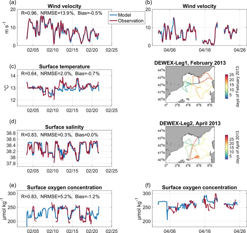
942                                        C. Ulses et al.: Oxygen budget of the north-western Mediterranean deep convection region

relation coefficient,                                                      3.1   Comparisons to cruise observations

           K                                                               The comparisons of modelled wind velocity and ocean model
       1
                 ykm − y m yko − y o
           P
       K                                                                   outputs with in situ observations from the high-frequency
           k=1
R=                                              ,                          SACES are shown in Fig. 2. Modelled wind provided by
                         σm σo                                             ECMWF and used to force the hydrodynamic model and to
                                                                           calculate the air–sea oxygen flux is highly correlated with
where K is the number of observations, yko is the observation              the observations (R = 0.96, p value < 0.01). The low val-
k, ykm is the corresponding model output k, and y o and y m are            ues of NRMSE (13.9 %) and percentage bias (−0.5 %) show
the mean of observations and model outputs, respectively; (3)              the accuracy of this variable, found for all ranges of value.
the normalised root-mean-square error,                                     Regarding the surface ocean variables, we obtain statistically
                 s                                                         significant correlations equal to 0.64, 0.83 and 0.83 (p value
                     1
                         K                 2                              < 0.01), between observed and modelled values of, respec-
                               yko − ykm
                         P
                     K                                                     tively, surface temperature, salinity and dissolved oxygen
                         k=1
NRMSE =                                         × 100 %;                   concentration. The NRMSEs are equal to 2.0 %, 0.3 % and
                               yo                                          5.2 %, respectively. The percentage biases remain negligible
                                                                           for temperature (−0.7 %), salinity (0.002 %) and dissolved
                                                      m    o
and (4) the percentage bias (PB = y y−y  o   × 100 %). The                 oxygen concentration (−1.2 %).
model results are compared with the observations at the same                  Figures 3 and 4 compare the observed and modelled dis-
dates and positions.                                                       solved oxygen concentration for the stations sampled dur-
                                                                           ing the DEWEX and MOOSE-GE cruises, respectively, at
                                                                           the surface (between 5 and 10 m) and along the south–north
                                                                           transect passing across the convection area (stations encir-
3     Evaluation of the model                                              cled in black in Fig. 3). Overall, the simulation correctly re-
                                                                           produces the spatial and temporal variability of the oxygen
The accurate representation of the winter mixing of water                  concentration observed at the surface and in the water col-
masses is an essential point for the simulation of the dis-                umn during and between the three cruises. During winter-
solved oxygen dynamics in this region, marked by a strong                  time, the model simulates low surface oxygen concentrations
ventilation of the deep waters that plays a crucial role in its            (< 220 µmol kg−1 ) in the open sea of the Gulf of Lion and the
seasonal cycle (Copin-Montégut et al., 2002; Touratier et al.,             Ligurian Sea, areas that coincide with the deep vertical mix-
2016; Coppola et al., 2017; 2018). A validation of the hy-                 ing regions (Estournel et al., 2016a; Kessouri et al., 2017)
drodynamic part of the simulation is described by Estour-                  (Fig. 3a and b). Figure 4a shows the oxygen homogenisa-
nel et al. (2016a), who showed similar spatial distribution of             tion of the whole water column between 41.5 and 42.3◦ N,
the modelled water column stratification in the entire deep-               the core of the deep-convection area. Concentrations above
convection area, as well as modelled time evolution of the                 240 µmol kg−1 are modelled in the surface layer on the shelf
temperature profile in the centre of the Gulf of Lion open sea             and in the south at the Balearic front, in accordance with the
during the winter that is close to the observations.                       observations (Figs. 3a, b and 4a). The model also agrees with
   Furthermore, an assessment of the biogeochemical part                   observations showing a layer of low oxygen concentration
of the coupled model is presented in Kessouri et al. (2017;                (minimum concentration < 185 µmol kg−1 at depths around
2018). These studies showed that the model is able to ac-                  500 m) located between 150 and 1500 m, mainly in the LIW
curately reproduce the timing and magnitude of the surface                 (300–800 m), outside the deep-convection area (Fig. 4a). The
chlorophyll increase during the spring and autumnal blooms,                metrics confirm the good agreement between model outputs
as well as the concentrations of nutrients and depths of nu-               and observations with a significant spatial correlation of 0.81
triclines and the dynamics and depth of the deep chlorophyll               and 0.61 (p value < 0.01), an NRMSE of 5.3 % and 15.7 %,
maximum during the stratified, oligotrophic period.                        and a negligible percentage bias of −1.1 % and 0.01 %, re-
   In this study, we focus the evaluation of the coupled model             spectively, at the surface and along the south–north transect.
on its ability to realistically represent the dynamics of dis-                During the spring cruise period, the model represents high
solved oxygen in the deep regions of the NW Mediterranean                  dissolved oxygen values (> 240 µmol kg−1 ) at the surface
Sea. For this purpose, we first compare the model results to               throughout the region, as observed (Fig. 3c and d). The in-
in situ observations from DEWEX and MOOSE-GE cruises                       crease in modelled oxygen concentration in the surface layer
conducted at three key periods: the winter mixing period, the              between both campaigns is in agreement with observations
phytoplankton bloom period and the stratified summer pe-                   (Figs. 3a–d and 4a, b). A zone of low oxygen concentra-
riod. We then compare the model outputs to Argo data de-                   tion in the intermediate waters is present in the convection
ployed in the area in terms of time evolution of oxygen in-                area in both datasets (Fig. 4b). However, it is worth noting
ventory.                                                                   that this zone of low oxygen concentration is heterogeneous

Biogeosciences, 18, 937–960, 2021                                                              https://doi.org/10.5194/bg-18-937-2021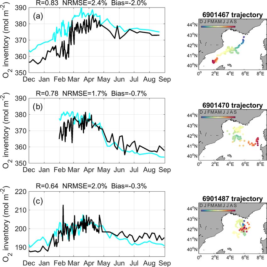
C. Ulses et al.: Oxygen budget of the north-western Mediterranean deep convection region                                                943

Figure 2. Time evolution during DEWEX Leg1 (in February 2013, a, c, d and e) and Leg2 (in April 2013, b, f) cruises of observed
(red) and modelled (blue) (a and b) wind velocity (m s−1 ), (c) surface temperature (◦ C), (d) surface salinity, and (e, f) surface dissolved
oxygen concentration (µmol kg−1 ). Trajectories of the measurements during DEWEX Leg1 and Leg2 cruises are indicated on inserted maps.
Modelled wind velocity was provided by ECMWF. No surface temperature and salinity data are available over the period of DEWEX Leg2.
The metrics indicated for the modelled wind velocity and surface oxygen concentration were calculated for both DEWEX Leg1 and Leg2
periods.

in its magnitude and thickness both in model outputs and                 cient of 0.64 and 0.96 (p value < 0.01), an NRMSE of 3.2 %
in observations, and it is not similarly distributed in space            and 3.5 %, and a negligible percentage bias (absolute values
in the model compared to the measurements. At the surface                ≤ 0.4 %) between model outputs and observations at the sur-
and along the transect, the spatial correlation coefficients be-         face and along the north–south transect, respectively.
tween modelled and observed dissolved oxygen are equal to                   The metrics computed using all station data from the three
0.59 and 0.30 (p value < 0.01), respectively, the NRMSE to               cruises are given in Table 1. The modelled dissolved oxygen
4.6 % and 19.3 %, respectively, and the percentage biases to             concentration is significantly correlated with the observed
−1.2 % and −4.4 %, respectively.                                         concentration (R ≥ 0.81, p < 0.01), in particular for the win-
   The north–south gradient, with lower surface concentra-               ter period when the pattern of the oxygen distribution appears
tions in the south of the deep-convection area, observed dur-            to be primarily shaped by deep-convection processes, shown
ing the stratified period (i.e. MOOSE-GE cruise period in                to be accurately represented by Estournel et al. (2016a). The
June–July), is then well reproduced by the model (Fig. 3e                model results show low percentage biases (PB < 1 %), low
and f). The minimum zone is more established than in spring              NRMSE (< 8 %), and SD ratios ranging between 1.13 and
in both in situ data and model results (Fig. 4c). Both sets              1.35, which indicate a larger variability in the observations
of data represent a maximum in the subsurface at depths                  than in the model outputs.
around 50 m, close to the deep chlorophyll maximum (shown
in Fig. 5 in Kessouri et al., 2018), although an underesti-
mation of its magnitude is visible between 41.5 and 42◦ N
in the model (Fig. 4c). We find a spatial correlation coeffi-

https://doi.org/10.5194/bg-18-937-2021                                                               Biogeosciences, 18, 937–960, 2021
944                             C. Ulses et al.: Oxygen budget of the north-western Mediterranean deep convection region

Figure 3. Surface dissolved oxygen concentration (µmol kg−1 ) observed (a, c and e) and modelled (b, d and f) over the (a and b) DEWEX
Leg1 (1–21 February 2013), (c and d) DEWEX Leg2 (5–24 April 2013) and (e and f) MOOSE-GE (11 June–9 July 2013) cruise periods.
The black-outlined dots correspond to the measurement stations shown in Fig. 4.

Table 1. Statistical analysis of model results: Pearson correlation coefficient (R), normalised root-mean-square error (NRMSE), percentage
bias (PB) and SD ratio, calculated between modelled dissolved oxygen concentrations and observations from DEWEX winter and spring
cruises and the MOOSE-GE summer cruise and from Argo-O2 platforms.

                                              R                             NRMSE, %       PB, %    SD ratio
                            DEWEX Leg1        0.86 (p < 0.01, n = 2960)             5.6    −0.59        1.34
                            DEWEX Leg2        0.93 (p < 0.01, n = 3960)             4.9     0.55        1.13
                            MOOSE 2013        0.81 (p < 0.01, n = 2960)             7.6     0.51        1.35
                            Float 6901467     0.56 (p < 0.01, n = 5120)            10.3    −0.12        1.37
                            Float 6901470     0.93 (p < 0.01, n = 4480)             3.0    −0.19        0.99
                            Float 6901487     0.88 (p < 0.01, n = 4720)             4.1    −0.11        1.01

3.2   Comparison to Argo float data                                    ≈ 10 mol m−2 over a layer from the surface to 1000 m, along
                                                                       the trajectory of the float 6901487 (Fig. 5c), both floats being
The model accurately reproduces the magnitude of oxygen                located in the Gulf of Lion at that period. The oxygen inven-
inventory in the water column and its time evolution ob-               tory remains high during the month of March and then de-
served using Argo floats during the study period (Fig. 5).             creases significantly from early April to early June, in model
The model simulates the increase observed between early                outputs and Argo observations. In both datasets, the decrease
December and late February. This increase is estimated at              reaches up to 20 mol m−2 over 1800 m along the path of the
≈ 20 mol m−2 over a layer from the surface to 1800 m,                  Argo float 6901470 in the Gulf of Lion (Fig. 5b) and is
along the trajectory of the float 6901467 (Fig. 5a), and at            less pronounced (≈ 10 mol m−2 ) along the trajectory of the

Biogeosciences, 18, 937–960, 2021                                                           https://doi.org/10.5194/bg-18-937-2021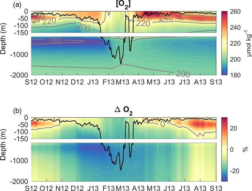
C. Ulses et al.: Oxygen budget of the north-western Mediterranean deep convection region                                             945

Figure 4. Comparison between model outputs and observations on a transect crossing the deep-convection area (stations are circled in black
in Fig. 3a, c and e) over the (a and b) DEWEX (Leg1: 10–12 February 2013, Leg2: 8–10 April) and (c) MOOSE-GE (27 June–5 July
2013) cruise periods. The left column shows observed and modelled profiles at 42 and 40.3◦ N. The right column shows vertical section
of dissolved oxygen concentration (µmol kg−1 ) along the transect; the model is represented by background colours and observations are
indicated in coloured circles.

float 6901467 in the Balearic Sea (Fig. 5a). More moder-               4   Atmospheric and hydrodynamic conditions
ate decreases are then simulated and observed until Septem-
ber along all float trajectories. The statistical analysis shows
that, in terms of oxygen inventory, significant correlation co-        In the NW Mediterranean Sea, deep convection takes place
efficients are obtained between the model outputs and the              every winter but shows strong interannual variability in its
three float observations (0.64 < R < 0.83, p value < 0.01),            magnitude and spatial extent. This interannual variability
NRMSEs are smaller than or equal to 2.4 %, and the abso-               is partly related to the variability of heat fluxes (Somot
lute values of percentage bias are smaller than or equal to            et al., 2016). Over the study period, the convection area
2 % (Fig. 5). In terms of dissolved oxygen concentration in            was marked by severe heat loss episodes from late Octo-
the water column, we obtain significant correlation coeffi-            ber 2012 to mid-March 2013 (Fig. 6a). In particular, there
cients (0.56 < R < 0.93, p value < 0.01), NRMSEs smaller               was a first short but intense heat loss event (mean heat flux
than 10.5 %, percentage biases smaller than 1 %, and SD ra-            < −1000 W m−2 ) at the end of October, followed by several
tios close to 1 for floats 6901470 and 6901487 and of 1.37             long northerly wind episodes when heat loss peaks reached
for float 6901467 (Table 1).                                           500 W m−2 , during the months of December to February
                                                                       (late November to mid-December, mid-January, early Febru-
                                                                       ary and late February). Finally, a last strong heat loss episode
                                                                       occurred in mid-March after a period of positive heat flux.
                                                                       The wind velocity averaged over the convection period (15

https://doi.org/10.5194/bg-18-937-2021                                                            Biogeosciences, 18, 937–960, 2021
946 C. Ulses et al.: Oxygen budget of the north-western Mediterranean deep convection region
Figure 5. The left column shows oxygen inventory integrated from the surface to 1800 m depth (a and b) or 1000 m (c) (mol m−2 ) in Argo
float measurements (cyan) and model outputs (black) along Argo (a) 6901467, (b) 6901470 and (c) 6901487 float trajectories. The right
column shows trajectories of corresponding Argo float.
January–8 March, 15–24 March) was maximum in the cen- central area of the Gulf of Lion, between 41.5 and 42.5◦ N
tre of the Gulf of Lion, where it reached 10 m s−1 (Fig. 7a). and 3.5 and 7◦ E and was smaller than 500 m in the Ligurian
From April onwards, the convection region was mainly char- Sea. From mid-April to the end of the period, the mixed layer
acterised by heat gains. was shallow (depth < 50 m) and its depth remained above the
In response to the autumnal heat loss events, the mixed nutriclines (Kessouri et al., 2017) and the deep chlorophyll
layer (ML) began to deepen below 50 m at the end of Novem- maximum (Kessouri et al., 2018).
ber (Fig. 6b). Its deepening was strongly enhanced in winter
over four periods that coincided with the four episodes of
intense northerly wind associated with heat loss mentioned 5 Results
above (Fig. 6a and b). Deep convection reached the bottom
layer (≈ 2000 m) in the core of the convection zone (latitude 5.1 Seasonal cycle of dissolved oxygen
≈ 42◦ N, 4◦ E < longitude < 5◦ E) in early February, and the
spatially averaged mixed layer reached a maximum depth of The good agreement found between model results and in
about 1500 m at the end of February (Fig. 6b). At the end situ measurements (Sect. 3) gave us confidence in the model
of the main convection event, end of February–early March, that we use here to analyse the evolution of the oxygen in-
the spatially averaged mixed layer abruptly decreased to less ventory in the deep-convection area and to quantify the rel-
than 100 m (Fig. 6b). Finally, during the secondary convec- ative contribution of each oxygen flux in its variation: ex-
tion event from 15 to 24 March, it reached almost 800 m. changes at the air–sea interface, as well as physical and bio-
Figure 7b shows the modelled mixed-layer depth (MLD) av- geochemical fluxes in the ocean interior. Based on the evo-
eraged over the convection periods. It exceeded 1000 m in a lution of vertical mixing and the phytoplankton growth in
the study area, Kessouri et al. (2017) divided the study pe-
Biogeosciences, 18, 937–960, 2021 https://doi.org/10.5194/bg-18-937-2021C. Ulses et al.: Oxygen budget of the north-western Mediterranean deep convection region 947
a deep chlorophyll maximum below 40 m depth (Kessouri et
al., 2018). In the following, we will analyse the dynamics of
dissolved oxygen for these four periods. The time evolution
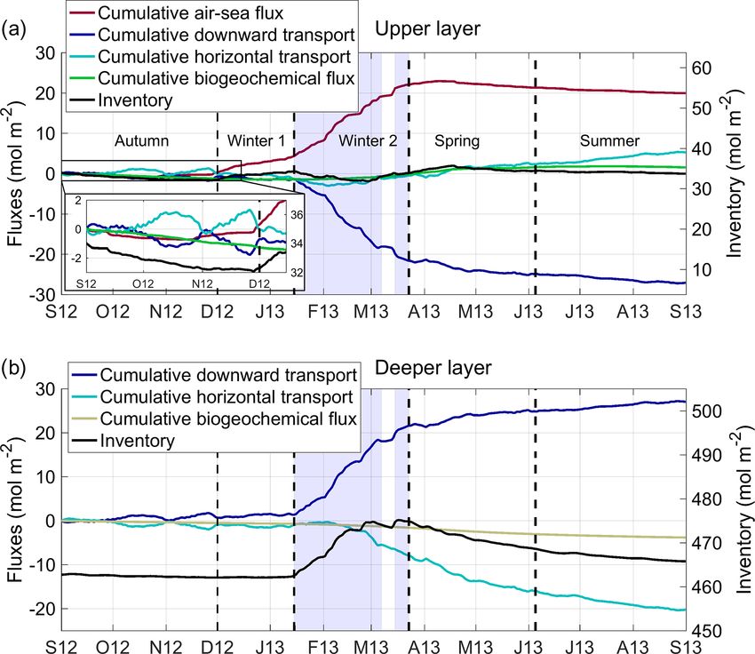
of daily oxygen budget terms is shown in Fig. 6d–f, while
the time evolution of cumulative oxygen fluxes and the re-
sulting variation in oxygen inventory for the upper (surface
to 150 m) and deeper (150 m to bottom) layers is presented in
Fig. 8. The biogeochemical term of the budget is defined as
the sum of oxygen production through photosynthesis and of
oxygen consumption through respiration by phytoplankton,
zooplankton and bacteria and through oxidation of ammo-
nium (nitrification) (see Eq. 1). The physical term is decom-
posed into two modes of transport: a net lateral transport due
to advection (positive values correspond to an input for the
deep-convection area) and a net vertical downward transport
at the interface between the two layers, at 150 m depth, due
to advection and turbulent mixing. Finally, the time evolution
of the dissolved oxygen concentration and the oxygen satu-
ration anomaly, 1O2 , averaged over the convection area is
shown in Fig. 9.
Autumn
From September to the end of November 2012 (91 d),
depth-integrated respiration exceeded depth-integrated pri-
Figure 6. Time series of modelled (a) total heat fluxes (W m−2 ), mary production in the upper layer (Fig. 6f). The result of
(b) mixed-layer depth (m), (c) surface oxygen and oxygen solu- biogeochemical processes in the water column was a net con-
bility (µmol kg−1 ), (d) air-to-sea oxygen fluxes (mmol m−2 d−1 ), sumption of oxygen and a decrease of 1.8 mol m−2 in oxygen
(e) downward oxygen transport at 150 m (dark blue) and lat- inventory (Fig. 8). Lateral transport was low for autumn and
eral oxygen transport towards the convection area (light blue) yielded a slight decrease of 0.9 mol m−2 in oxygen inventory
(mmol m−2 d−1 ), and (f) biogeochemical oxygen production (see (Fig. 8). The heat loss and vertical mixing caused by the
Eq. 1) (mmol m−2 d−1 ), spatially averaged over the convection northerly wind gust at the end of October 2012 led to a de-
area (spatial mean in solid line and shaded area for SD). Sources:
crease in surface temperature and consequently to an increase
ECMWF for heat fluxes, SYMPHONIE/Eco3M-S for the other pa-
rameters and fluxes. The blue shaded area corresponds to the deep-
in oxygen solubility (Fig. 6c). In addition, the vertical mix-
convection period (period when spatially averaged MLD > 100 m). ing reached the depth of the oxygen maximum present in the
Note that the range of the y axis varies for the different oxygen subsurface (Fig. 9). This caused its erosion and an increase in
fluxes, and due to higher values SD for vertical and lateral transport the surface oxygen concentration which was, however, lower
is not shown. than the oxygen solubility (Figs. 9 and 6c). From this event,
the NW deep-convection area became undersaturated at the
surface (Fig. 9b) and the sea began to absorb atmospheric
riod into four sub-periods. The first period from September oxygen (flux towards the ocean of 80 mmol d−1 on 29 Octo-
to the end of November, which we will refer to as the autumn ber, Fig. 6d). Over the autumnal period, the cumulative air–
period, is characterised by a stratified water column (mean sea oxygen flux amounted to 0.3 mol m−2 (Fig. 8a). Globally,
MLD < 50 m) and respiration dominating primary produc- the convection area was characterised by a decrease in oxy-
tion (Kessouri et al., 2018). The second period, from the end gen inventory of 2.4 mol m−2 , more than two-thirds of which
of November to the end of March, referred to here as the occurred in the upper layer.
winter period, is characterised by a sustained vertical mix-
ing (mean MLD > 50 m). The third period, called spring, ran Winter
from late March to early June. It corresponds to the period of
restratification of the water column (Estournel et al., 2016a) The winter period was defined from late November 2012
and of the peak of the phytoplankton bloom at the sea sur- to late March 2013 but can be further divided into two
face followed by the formation of a deep chlorophyll maxi- sub-periods based on the intensity of the vertical mixing
mum (Kessouri et al., 2018). The last period, summer, from (Kessouri et al., 2017). During the first sub-period, from
early June to September, is characterised by a strong stratifi- the end of November to mid-January (44 d), the mixing in-
cation (mean MLD < 20 m) and the permanent presence of tensified, but remained moderate: the ML averaged over
https://doi.org/10.5194/bg-18-937-2021 Biogeosciences, 18, 937–960, 2021948 C. Ulses et al.: Oxygen budget of the north-western Mediterranean deep convection region
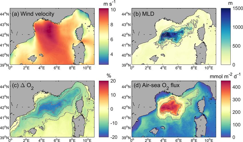
Figure 7. Modelled (a) wind velocity (m s−1 ), (b) mixed-layer depth (m) (dark grey lines represent 500, 1000 and 1500 isocontours and
light grey line the contour of the deep-convection area), (c) oxygen saturation anomaly (%) at the surface and (d) air-to-sea oxygen flux
(mmol m−2 d−1 ), averaged over the 2013 deep-convection period (15 January–8 March; 15–24 March).
Figure 9. Time evolution of (a) the dissolved oxygen concentra-
tion (µmol kg−1 ) and (b) the oxygen saturation anomaly (%), with
Figure 8. Time series from September 2012 to September 2013 of mixed-layer depth (m) indicated by the black line, all horizontally
the oxygen inventory (black line) and cumulative air–sea flux (red averaged over the deep-convection area.
line), downward transport (dark blue), lateral transport (positive val-
ues: input for the convection area, light blue), and biogeochemical
flux (green line) in the (a) upper (surface to 150 m) and (b) deeper itive in the upper layer (Fig. 6f). However, over this sub-
(150 m to bottom) layer. Unit: mol m−2 . period, the influence of biogeochemical processes on the
oxygen inventory remained low (−0.3 mol m−2 , Fig. 8). Air-
to-sea oxygen flux was marked by several peaks, greater than
the deep-convection area remained above the depth of the 250 mmol m−2 d−1 (Fig. 6d), coinciding with cold gales from
maximum euphotic layer (150 m; see Sect. 2.1.3) (Fig. 9). the north. Its contribution to the oxygen inventory over this
The vertical mixing induced a supply of inorganic nutri- sub-period amounted to 3.6 mol m−2 . Regarding the lateral
ents in the upper layer that supported primary production. oxygen export, it contributed to a loss of 1.3 mol m−2 . The
Kessouri et al (2018) identified the beginning of this pe- sum of the contributions of the different processes in the wa-
riod as the beginning of a first bloom. From mid-December, ter column and at the air–sea interface yielded an increase in
the net biogeochemical production of oxygen became pos- O2 inventory of 2.0 mol m−2 in the water column. A total of
Biogeosciences, 18, 937–960, 2021 https://doi.org/10.5194/bg-18-937-2021C. Ulses et al.: Oxygen budget of the north-western Mediterranean deep convection region 949 90 % of this increase occurred in the upper layer, from which phytoplankton or horizontally advected in the upper layer, 0.7 mol m−2 of O2 was exported toward the deeper layers. was massively transported to the intermediate and deep lay- The second winter sub-period, from mid-January to late ers (20.1 mol m−2 ). It is worth noting that vertical fluxes March (69 d), corresponds to the period of deep convec- showed high spatial variability within the convection area. tion. From the middle to the end of January, the surface Over this period, the lateral transport from the aphotic layer water masses previously enriched with oxygen, due to pri- outside the convection area represents 33 % of the amount mary production and air–sea exchanges, were mixed with of downward transport. Globally, the different contributions the intermediate water masses characterised by a minimum led to an increase in the water column oxygen inventory of of oxygen (Fig. 9). From the beginning of February, the ver- 12.3 mol m−2 . tical mixing intensified, causing a net oxygen transport to- wards deeper layers (depth > 800 m, Figs. 6e, 8 and 9). O2 Spring (late March to early June, 74 d) concentration decreased significantly at the surface and the difference between surface oxygen concentration and oxy- In spring, net biogeochemical production of O2 remained gen solubility deepened further, with the oxygen saturation high in the upper layer until the bloom peak in mid-April; anomaly reaching −15 % until the end of the convection pe- afterwards it decreased but generally remained positive until riod (Fig. 9). Over this sub-period, the whole NW convec- the end of that period (Fig. 6f). Oxygen consumption through tion area was undersaturated at −10 % to −15 % (Fig. 7c). heterotrophic respiration in the deeper layers also remained Strong undersaturation and wind intensity led to very high relatively high. The result of biogeochemical contributions air–sea fluxes. Several peaks reaching 800 mmol m−2 d−1 are was a small increase of 0.3 mol m−2 in the O2 inventory of modelled until mid-March (Fig. 6d). The contribution of the water column. air–sea fluxes over this period amounted to 18.0 mol m−2 During this period, primary production led to a sharp (Fig. 8a). Over the deep-convection period, air–sea oxy- increase in surface oxygen concentration from 220 to gen exchanges are characterised by high spatial variability 280 µmol kg−1 at the peak of the phytoplankton bloom (Fig. 7d) with a SD of 38 %. The air-to-sea oxygen flux av- (Fig. 6c), and the latter became above saturation in early eraged over the deep-convection period varied between 300 April, when the convection area became a source of oxygen and 460 mmol m−2 d−1 in the heart of the convection area for the atmosphere (Fig. 6c and d). This oversaturation situ- and between 65 and 200 mmol m−2 d−1 in the Ligurian Sea. ation at the surface then persisted until the end of the period. With regard to biogeochemical processes, as shown in pre- The model simulates significant outgassing during the bloom vious studies (Auger et al., 2014; Kessouri et al., 2018), zoo- peak (235 mmol m−2 d−1 on 18 April 2013, Fig. 6d) when plankton growth was largely reduced by the deep-convection the mean saturation anomaly reached a maximum value of process due to a dilution-induced decoupling of prey and 15 % (Figs. 6c and 9). Overall, the convection area released predators. In the upper layer, oxygen production through pri- 0.8 mol m−2 of oxygen to the atmosphere during spring. Dur- mary production exceeded oxygen consumption processes ing this restratification phase, a moderate oxygen export to (respiration, nitrification) (Fig. 6f). In parallel, the export of the deep layers is found (3.2 mol m−2 , Fig. 8). Lateral ex- organic matter into the intermediate and deep layers dur- port to regions surrounding the convection area continued at ing deep convection (Kessouri et al., 2018) led to an in- a high rate with a cumulative value of 5.1 mol m−2 . Finally, crease in remineralisation processes (Fig. 6f) and conse- over this period, the water column in the convection area was quently a decrease in oxygen inventory in these aphotic lay- subjected to a 5.7 mol m−2 decrease in its oxygen inventory, ers. The sum of biogeochemical fluxes over the entire water due to the lateral export of oxygen via the spreading of dense column resulted in a small increase in oxygen inventory of waters in the deeper layers and a slight outgassing to the at- 0.4 mol m−2 , negligible compared to that induced by air–sea mosphere. fluxes, in consistency with the previous study of Minas and Bonin (1988). Summer Over this period, the lateral export of dissolved oxygen had high values, reaching 220 mmol m−2 d−1 (Fig 6e). In the During the summer period (87 d), the surface oxygen concen- upper layer, the total lateral transport over the period was low tration remained higher than the oxygen solubility (Fig. 6c). (0.5 mol m−2 ), while it is estimated that in the deeper layers A supersaturated situation occurred in the deep chloro- 6.7 mol m−2 was exported horizontally from the convection phyll maximum zone, due to primary production and a gen- area between mid-February and the end of the convection pe- eral stratification (Fig. 9). We estimate that the ocean re- riod (Fig. 8b). The downward transport at the base of the up- leased 1.4 mol O2 m−2 to the atmosphere over this period per layer showed strong peaks reaching 500 mmol m−2 d−1 (Fig. 8), mainly during moderate northerly gales. Depth- (Fig. 6e), concomitant with the peaks of the air-to-sea fluxes integrated oxygen-consuming biogeochemical processes ex- and the deepening of the ML. ceeded depth-integrated primary production on average over The model results indicate that atmospheric oxygen in- this period. The result of biogeochemical fluxes was re- jected at the surface and, to a lesser extent, produced by sponsible for a consumption of 0.8 mol m−2 of oxygen. https://doi.org/10.5194/bg-18-937-2021 Biogeosciences, 18, 937–960, 2021
950                                 C. Ulses et al.: Oxygen budget of the north-western Mediterranean deep convection region

                                                                            ward the bottom occurred during 68 % of the events of deep
                                                                            vertical mixing of oxygen-rich surface waters with oxygen-
                                                                            poor underlying waters. Finally, the budget shows that the
                                                                            deep-convection area appears as a net source for dissolved
                                                                            oxygen for the rest of the western Mediterranean Sea with
                                                                            an annual net horizontal transport of 15.0 mol O2 m−2 . This
                                                                            transport breaks down into an input of 5.3 mol O2 m−2 in the
                                                                            upper layer and an export of 20.3 mol O2 m−2 in the deeper
                                                                            layer.
                                                                               At the end of the annual cycle, a negligible decrease
                                                                            (0.3 mol m−2 , i.e. 0.05 %) in the oxygen inventory of the up-
                                                                            per euphotic layer is found, while 3.1 mol m−2 (i.e. 0.66 % of
                                                                            the inventory) was stored in the deeper water masses.

Figure 10. Schematic showing the terms of the annual oxygen                 6     Discussion
budget (mol O2 m−2 ) for the north-western Mediterranean deep-
convection area over the period from September 2012 to September
                                                                            6.1    Air–sea oxygen flux
2013. FA–S : air-to-sea flux; FH : net horizontal transport; Fv 150 : net
downward transport at the base ofRthe euphotic layer (150 m); FB :
net biogeochemical production; 1 O2 : variation in oxygen inven-
                                                                            Our model results indicate that the NW Mediterranean deep-
tory. Positive fluxes are inputs for the deep-convection zone. The          convection area was a net sink for the atmospheric oxy-
terms of the budget are estimated for the upper euphotic layer (sur-        gen at a rate of 20.0 mol m−2 yr−1 between September 2012
face to 150 m) and the deeper aphotic layers (150 m to bottom).             and September 2013 and at a rate of 280 mmol m−2 d−1
                                                                            (17.7 mol m−2 over 63 d) during the 2013 deep-convection
                                                                            period. Inside the area, the annual air–sea flux shows
In addition, the convection area continued to export oxy-                   strong spatial heterogeneity, with a range extending from
gen to the adjacent zone (1.3 mol m−2 ), but at a lower                     2.7 mol m−2 yr−1 at the periphery to 36.0 mol m−2 yr−1 in
rate (15 mmol m−2 d−1 ) than in the two previous peri-                      the centre. Considering its sea surface area (61 720 km2 ),
ods (90 mmol m−2 d−1 over the deep-convection period and                    the NW deep-convection zone received 1233 Gmol of oxy-
69 mmol m−2 d−1 in spring). Finally, the oxygen inventory                   gen from the atmosphere over the period September 2012
decreased by 3.5 mol m−2 in the whole water column of the                   to September 2013, including 1090 Gmol during the win-
deep-convection area (Fig. 8).                                              ter 2013 intense vertical mixing period. We showed that the
                                                                            strong oxygen ingassing was essentially driven by a high un-
5.2   Annual oxygen budget                                                  dersaturation (< −10 %) and intense northerly winds during
                                                                            the deep-convection period.
Figure 10 illustrates the oxygen budget of the NW Mediter-                     Nevertheless, uncertainties in the net uptake rate remain.
ranean convection area over the period September 2012 to                    First, uncertainties are linked to errors in modelled ocean
September 2013. At the annual scale, the deep-convection                    surface variables (dissolved oxygen, temperature and salin-
area is a net sink of oxygen for the atmosphere, estimated at               ity) and wind velocity used for the calculation of the air–
20.0 mol O2 m−2 . A total of 88 % (17.7 mol O2 m−2 ) of this                sea flux. The comparisons of model results with in situ high-
amount was injected into the ocean interior during the period               frequency measurements at the surface during the period of
when the deep-convection process took place.                                maximum flux (deep-convection period) indicate a bias of
   The annual net biogeochemical production of oxygen in                    less than or close to 1 % and a NRMSE smaller than 14 %
the euphotic layer (0–150 m) is estimated at 1.6 mol O2 m−2 .               for the wind velocity, surface temperature, salinity and oxy-
The net annual NCP (net community production, defined                       gen concentration (Sect. 3.1). A second source of uncer-
as gross primary production minus community respiration                     tainty is linked to the parameterisation chosen for the cal-
in the euphotic zone) is estimated at 3.9 mol O2 m−2 yr−1 ,                 culation of the gas transfer velocity. In the standard run, we
yielding autotrophy in this area. In the deeper layers (150 m–              used the cubic dependence with wind speed parameterisa-
bottom) an oxygen consumption of 3.8 mol O2 m−2 was as-                     tion proposed by Wanninkhof and McGillis (1999). Sensitiv-
sociated with respiration of heterotrophic organisms by 70 %                ity analyses were performed using eight other parameterisa-
and oxidation of ammonium by 30 %. This led to an annual                    tions for the calculation of air–sea flux (Wanninkhof, 1992,
net biogeochemical consumption of 2.2 mol O2 m−2 over the                   2014; Woolf, 1997; Nightingale et al., 2000; Wanninkhof et
whole water column.                                                         al., 2009; Stanley et al., 2009; Liang et al., 2013; Bushin-
   The model indicates that 27.1 mol m−2 of O2 was exported                 sky and Emerson, 2018; see Sect. 2.1.2). Estimates of annual
from the upper layer to deeper layers. This net transport to-               air–sea flux, as well as flux and amount of atmospheric oxy-

Biogeosciences, 18, 937–960, 2021                                                              https://doi.org/10.5194/bg-18-937-2021
You can also read