Haplo-diplontic life cycle expands coccolithophore niche
←
→
Page content transcription
If your browser does not render page correctly, please read the page content below
Biogeosciences, 18, 1161–1184, 2021
https://doi.org/10.5194/bg-18-1161-2021
© Author(s) 2021. This work is distributed under
the Creative Commons Attribution 4.0 License.

Haplo-diplontic life cycle expands coccolithophore niche
Joost de Vries1,2 , Fanny Monteiro1 , Glen Wheeler2 , Alex Poulton3 , Jelena Godrijan4 , Federica Cerino5 ,
Elisa Malinverno6,7 , Gerald Langer2 , and Colin Brownlee2,8
1 BRIDGE,   School of Geographical Sciences, University of Bristol, University Road, Bristol BS8 1SS, UK
2 Marine Biological Association, The Laboratory, Citadel Hill, Plymouth PL1 2PB, UK
3 The Lyell Centre for Earth & Marine Science & Technology, Heriot-Watt University, Edinburgh EH14 4BA, UK
4 Division for Marine and Environmental Research, Rud̄er Bošković Institute, Bijenička cesta 54, 10000 Zagreb, Croatia
5 Oceanography Section, Istituto Nazionale di Oceanografia e di Geofisica Sperimentale – OGS,

via Piccard 54, 34151 Trieste, Italy
6 Department of Earth and Environmenal Sciences, University of Milano-Bicocca,

Piazza della Scienza 4, 20126 Milan, Italy
7 Consorzio Nazionale Interuniversitario per le Scienze del Mare – CoNISMa, Piazzale Flaminio 9, 00196 Rome, Italy
8 School of Ocean and Earth Science, University of Southampton, Southampton SO14 3ZH, UK

Correspondence: Joost de Vries (joost.devries@bristol.ac.uk)

Received: 26 May 2020 – Discussion started: 24 June 2020
Revised: 29 October 2020 – Accepted: 22 November 2020 – Published: 16 February 2021

Abstract. Coccolithophores are globally important marine         derstanding of coccolithophore ecology. Our results further-
calcifying phytoplankton that utilize a haplo-diplontic life     more suggest a different response to nutrient limitation and
cycle. The haplo-diplontic life cycle allows coccolithophores    stratification, which may be of relevance for further climate
to divide in both life cycle phases and potentially expands      scenarios.
coccolithophore niche volume. Research has, however, to             Our compilation highlights the spatial and temporal spar-
date largely overlooked the life cycle of coccolithophores and   sity of SEM measurements and the need for new molecular
has instead focused on the diploid life cycle phase of coc-      techniques to identify uncalcified haploid coccolithophores.
colithophores. Through the synthesis and analysis of global      Our work also emphasizes the need for further work on the
scanning electron microscopy (SEM) coccolithophore abun-         carbonate chemistry niche of the coccolithophore life cycle.
dance data (n = 2534), we find that calcified haploid coc-
colithophores generally constitute a minor component of the
total coccolithophore abundance (≈ 2 %–15 % depending on
season). However, using case studies in the Atlantic Ocean       1   Introduction
and Mediterranean Sea, we show that, depending on en-
vironmental conditions, calcifying haploid coccolithophores      Coccolithophores are marine phytoplankton that produce
can be significant contributors to the coccolithophore stand-    calcium carbonate platelets, called “coccoliths”, which can
ing stock (up to ≈ 30 %). Furthermore, using hypervolumes        be seen from space when coccolithophores bloom. Coccol-
to quantify the niche of coccolithophores, we illustrate that    iths eventually rain down into the ocean interior or serve as
the haploid and diploid life cycle phases inhabit contrasting    ballast as they are incorporated into faecal pellets and ag-
niches and that on average this allows coccolithophores to       gregates, which drives the carbonate pump and enhances the
expand their niche by ≈ 18.8 %, with a range of 3 %–76 %         organic carbon pump by increasing organic carbon export
for individual species.                                          rates to the deep sea (Klaas and Archer, 2002; Zeebe, 2012).
   Our results highlight that future coccolithophore research    Through the production of coccoliths, coccolithophores pro-
should consider both life cycle stages, as omission of the       duce ≈ 1.5 Pg of inorganic carbon per year (Hopkins and
haploid life cycle phase in current research limits our un-      Balch, 2018; Krumhardt et al., 2019) and subsequently ac-
                                                                 count for 30 % to 90 % of carbonate in sediments (Broecker

Published by Copernicus Publications on behalf of the European Geosciences Union.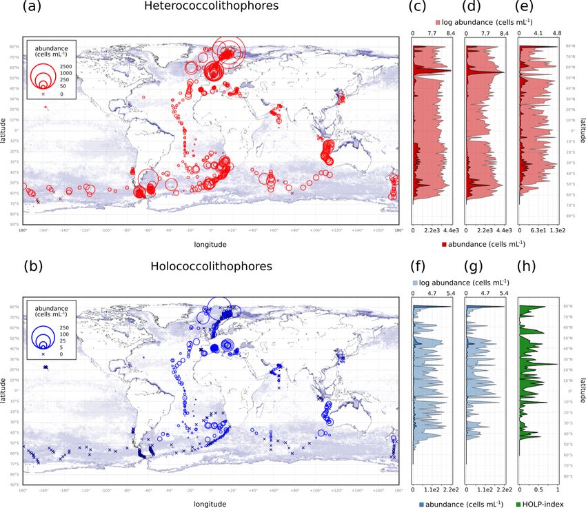
1162                                                 J. de Vries et al.: Haplo-diplontic life cycle expands coccolithophore niche

and Clark, 2009), highlighting the importance of coccol-
ithophores in calcium carbonate burial.
   In addition to the carbonate pump, coccolithophores con-
tribute to the organic carbon pump, accounting for 1 %–40 %
of marine primary production depending on habitat (Poulton
et al., 2007, 2013). Because of involvement in the ocean car-
bon pumps and food web, coccolithophores thus play an im-
portant role in the ocean on regional to global spatial scales
and seasonal to geological timescales.
   Much focus has been put on understanding coccol-
ithophore ecology and physiology, such as the function of
calcification (Young, 1994; Monteiro et al., 2016; Xu et al.,
2016), their diversity (Aubry, 2009; Young et al., 2003), and
the factors controlling their calcification (Zondervan, 2007;
Taylor et al., 2017) and competitiveness (Margalef, 1978;
Krumhardt et al., 2017). However, one factor that signifi-
cantly impacts coccolithophore calcite production and poten-
tially their global success has been given little attention: their
distinctive life cycle.
   The life cycle of an organism is defined by the number of
                                                                       Figure 1. Life cycle strategies of phytoplankton: (a) dinoflagellates
chromosome sets (the “ploidy level”) of the cell when asex-
                                                                       tend to utilize a haplontic life cycle, (b) diatoms tend to utilize a
ual reproduction (“mitosis”) occurs. If mitosis occurs when
                                                                       diplontic life cycle, and (c) coccolithophores tend to utilize a haplo-
the cell has one set of chromosomes (a haploid cell) the life          diplontic life cycle. Note that not all coccolithophores calcify in
cycle is called “haplontic” (Fig. 1a), while if mitosis occurs         their haploid phase.
when the cell has two sets of chromosomes (a diploid cell)
the life cycle is called “diplontic” (Fig. 1b). A few organisms
can divide in both the haploid and diploid phase. Such a life
cycle is called “haplo-diplontic” (Fig. 1c). Coccolithophores          quently utilized (Frada et al., 2018). Eight coccolithophore
utilize the latter life cycle strategy – which is in contrast to di-   clades utilize holococcoliths, while four clades utilize an un-
noflagellates and diatoms, which tend to be either haplontic           mineralized haploid morphology, one clade utilizes a cera-
or diplontic and as such can only divide in either the hap-            tolith morphology, and one clade utilizes ceratolith morphol-
loid or diploid life cycle phase (Von Dassow and Montresor,            ogy, while for five clades the haploid morphology is currently
2011).                                                                 unknown (Frada et al., 2018).
   The haploid and diploid life cycle phases of coccol-                   Coccolith and coccosphere morphology, cell and cocco-
ithophores can vary significantly in terms of coccolith struc-         sphere size, and the degree of calcification influence coccol-
ture, size, and morphology; cell size; and degree of calcifi-          ithophore ecology (Young, 1994). We can thus expect that
cation (Fig. 2). The diploid life cycle phases tend to be more         the haploid and diploid life cycle phases of coccolithophores
heavily calcified than the haploid life cycle phases, which            can have contrasting ecological preferences, which might
tend to be more lightly or non-calcified (Cros et al., 2000;           allow a coccolithophore species to occupy multiple niches
Daniels et al., 2016; Fiorini et al., 2011a, b). This difference       (Houdan et al., 2006; Frada et al., 2012; Cros and Estrada,
in cell calcium carbonate content (particulate inorganic car-          2013; Godrijan et al., 2018; Frada et al., 2018). This abil-
bon, PIC), cell organic carbon content (particulate organic            ity to occupy multiple niches should expand the total niche
carbon, POC) and the ratio thereof (the PIC : POC ratio) be-           coccolithophore can inhabit, a potential advantage for haplo-
tween the two life cycle phases means that the two phases              diplontic organisms in variable environments (Mable and
potentially have contrasting impacts on the carbonate pump.            Otto, 1998). This is an idea that is supported by genetic mod-
   Although coccolithophore morphology is highly diverse,              els (Hughes and Otto, 1999; Rescan et al., 2015).
the diploid phases of coccolithophores primarily utilize                  While niche differentiation has been widely observed for
heterococcolithophore morphology (with some exceptions,                haplo-diplontic seaweeds (Couceiro et al., 2015; Guillemin
i.e. Braarudosphaera bigelowii), while the haploid life cy-            et al., 2013; Lees et al., 2018; Lubchenco and Cubit, 1980)
cle phases can broadly be classified into four morpholo-               and coccolithophores (Houdan et al., 2006; Cros and Estrada,
gies: polycrater (Fig. 2a), ceratolith (Fig. 2b), holococcolith        2013; Godrijan et al., 2018; Frada et al., 2018), to date no
(Fig. 2c–i), and unmineralized (not pictured) (Frada et al.,           research has quantitatively investigated the extent of niche
2018). Of these four haploid morphologies, the holococcol-             overlap and niche expansion for haplo-diplontic algae. For
ithophore morphology – which is defined by rhomboid cal-               coccolithophores this is because research has primarily fo-
cite structures that constitute the coccoliths – is the most fre-      cused on the diploid life phases, and relatively little is known

Biogeosciences, 18, 1161–1184, 2021                                                         https://doi.org/10.5194/bg-18-1161-2021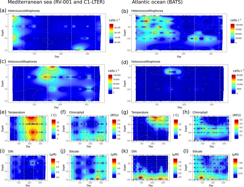
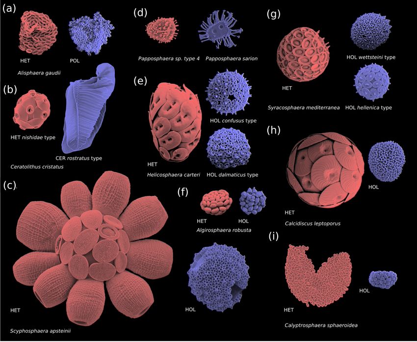
J. de Vries et al.: Haplo-diplontic life cycle expands coccolithophore niche                                                          1163

Figure 2. Coccosphere diversity of common coccolithophores (haploid cells are coloured in blue and diploid cells in red): (a) polycrater
haploid morphology, (b) ceratolith haploid morphology, and (c–i) holococcolith haploid morphology. Note that in some instances multiple
haploid phases are associated with one diploid phase (e.g. Syracosphaera mediterranea and Helicosphaera carteri), which may be due to
cryptic speciation (Geisen et al., 2002). Furthermore, some species (e.g. E. huxleyi) do not calcify in their haploid phase and are thus not
pictured. Images reproduced with permission from Young et al. (2020) (b–d, i) and Šupraha et al. (2016) (a, e–h). Panels (b)–(d) and (i)
(HOL) were created by Jeremy Young, (i) (HET) was created by Marie-Helene Kawachi, and (a) and (e)–(h) were created by Luka Šupraha.

in regard to the haploid life phase (Taylor et al., 2017; Frada         clades rather than E. huxleyi, holococcolith-forming clades
et al., 2018). This is in part due to a research focus on               include ecologically relevant species such as Helicosphaera
the globally ubiquitous Emiliania huxleyi, which utilizes an            carteri (Fig. 2e), Coccolithus pelagicus, and Calcidiscus lep-
unmineralized haploid morphology that cannot be readily                 toporus (Fig. 2h), which contribute more to the CaCO3 flux
identified with conventional light or scanning electron mi-             to the deep ocean than E. huxleyi due to their larger coccolith
croscopy (Frada et al., 2008).                                          and coccosphere size (Ziveri et al., 2007; Rigual Hernández
   With the aim of understanding how haploid coccol-                    et al., 2019).
ithophores contribute to coccolithophore success, we quan-                 In addition to niche overlap and niche expansion, we in-
tify the niche overlap and niche expansion between haploid              vestigate the data set to identify ecological preferences of
and diploid life stages of coccolithophores for the first time.         holococcolith-forming species, providing an updated picture
   To do so, we compile global coccolithophore abundance                on their global distribution, relative abundance, niche, and
observations of coccolithophores using all available scanning           environmental controls. This work provides key information
electron microscopy (SEM) measurements and where appro-                 to better understand how the haplo-diplontic life cycle con-
priate corresponding environmental measurements (temper-                tributes to coccolithophore success.
ature, salinity, dissolved inorganic nitrogen, phosphate, and
silicate). Although our focus is on holococcolith-forming

https://doi.org/10.5194/bg-18-1161-2021                                                          Biogeosciences, 18, 1161–1184, 2021
1164                                              J. de Vries et al.: Haplo-diplontic life cycle expands coccolithophore niche

2     Methods                                                         All data were acquired from supplementary data, online
                                                                   databases, or by contacting the authors directly if neither
2.1    Metadata compilation                                        of these methods were available. The data were manually
                                                                   checked for synonyms or misspellings of species names,
Coccolithophore abundance measurements were compiled               and where appropriate cell abundances were converted to
from 36 studies, constituting 2534 measurements and rep-           cells L−1 . All species (or genera if not identified to a species
resenting all major oceans (Table 1). These studies utilized       level) were labelled as either heterococcolithophore, holo-
scanning electron microscopy (SEM) to enumerate or fur-            coccolithophore, or “other”, which includes polycrater, nano-
ther identify coccolithophores rather than solely relying on       liths, and unidentified species. For these categorizations we
the more commonly utilized light or cross-polarized mi-            followed definitions from Cros and Fortuño (2002).
croscopy which under-represents coccolithophore biodiver-             The species and environmental data were compiled in
sity (Godrijan et al., 2018), especially in the case of holococ-   Python and subsequently analysed in R (R Core Team,
colithophores (Bollmann et al., 2002; Cerino et al., 2017).        2019). For all analyses we only considered samples within
We used this data set to investigate global and vertical dis-      the top 200 m of the water column. To reduce the effects
tribution patterns of haploid and diploid coccolithophore life     of seasonality, we binned the data into four main seasons,
cycle phases, specifically focusing on holococcolith forming       defined as December–February, March–May, June–August,
species. Since abundance data were manually compiled, our          September–November. We also calculated the mean of the
data set is not exhaustive. For instance, some SEM studies,        observed abundances on a global scale and regional scale and
such as those by Okada and Honjo (1973), Honjo and Okada           estimated the highest observed abundances (the “maximum
(1974), and Reid (1980), are not included in this data set         abundance”) for both heterococcolithophores and holococ-
since the data were not retrievable from the original publi-       colithophores and for each season. For the mean abundance
cations.                                                           calculations the mean was calculated for each sample and
   In addition to the global data set, we further investi-         then averaged. Finally, we tested the count data for a normal
gated three case studies in order to better understand spe-        distribution using a Shapiro–Wilk test for each region and the
cific drivers and differences between the life cycle phases:       global data set. Where the count distribution was found to be
the Atlantic Meridional Transect (AMT), representative             normal (all data), a 95 % confidence interval was calculated.
of mid-oligotrophic open-ocean ecosystems; the long-term
time series at Bermuda (BATS); and two time series in              Sampling bias and cover of data set
a mesotrophic coastal ecosystem in the Adriatic Sea (the
“Mediterranean data set”). For the AMT study, we con-              Our compilation contains sampling bias and is spatially and
sidered observations from four cruises, specifically AMT-          temporally incomplete. Temporally, there is bias towards the
12 (May–June 2003), AMT-14 (April–June 2004), AMT-                 months June–August and December–February (29.28 % and
15 (September–October 2004), and AMT-17 (October–                  30.59 % of samples, respectively), with fewer samples in
November 2005), which had been previously published by             the inter-seasons. This temporal bias results from generally
Poulton et al. (2017). For the BATS station we considered          higher sampling effort in the Arctic Circle in June–August
data published by Haidar and Thierstein (2001), which con-         (8.43 % of samples) and the Southern Ocean in December–
sists of approximately monthly observations between Jan-           February (13.15 % of samples). Not coincidentally, this is
uary 1991 and January 1994. For the Mediterranean study,           when and where coccolithophore abundances are the highest
we combine two time series in the Adriatic Sea by Godrijan         (see results below). When excluding the Arctic Circle (June–
et al. (2018) and Cerino et al. (2017) taken between Septem-       August) and the Southern Ocean (December–February), the
ber 2008 to December 2009 and May 2011 to February 2013            data set is temporally relatively evenly distributed (28.20 %
at the RV-001 and C1-LTER stations, respectively.                  March–May, 26.58 % June–August, 22.13 % September–
   For the BATS, AMT, and Mediterranean case studies, we           November, 22.23 % December–February).
additionally compiled temperature; salinity; and concentra-           Spatially, there is higher sampling in the Atlantic Ocean,
tions of dissolved inorganic nitrogen (DIN; nitrite + nitrate),    Mediterranean Sea, Arctic Circle, and Southern Ocean. In
phosphate, and silicate. For the AMT studies, environmen-          terms of spatial cover, coverage is limited in the Pacific
tal variables were acquired from the British Oceanographic         Ocean and data is lacking in the Southern Ocean between
Data Centre (BODC). For the BATS studies, environmental            June–August and the Arctic Circle between Dec–May. How-
variables were acquired from the Bermuda Institute of Ocean        ever, previous studies note the low coccolithophore abun-
Sciences (BIOS). For the Mediterranean study, day length           dance in the tropical and subtropical Pacific Ocean (Okada
was calculated using the MIT Skyfield package in Python.           and Honjo, 1973; Honjo and Okada, 1974; Reid, 1980), and
Other environmental variables such as turbulence, irradiance,      the absence or low abundance of holococcolithophores in this
and pH might also impact coccolithophore distribution pat-         region (Okada and Honjo, 1973; Honjo and Okada, 1974;
terns, but we have not included them in our compilation be-        Reid, 1980). The lack of data in the Southern Ocean and the
cause they are not available for all presented case studies.       Arctic Circle for specific months is due to the difficulty of

Biogeosciences, 18, 1161–1184, 2021                                                   https://doi.org/10.5194/bg-18-1161-2021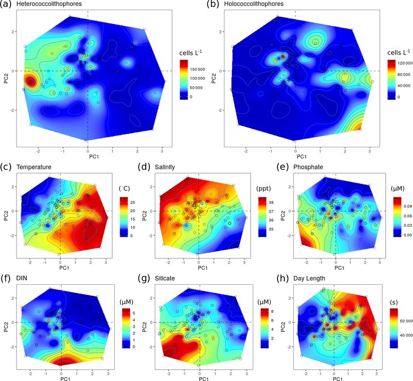
J. de Vries et al.: Haplo-diplontic life cycle expands coccolithophore niche                                                        1165

Table 1. Overview of metadata. The following abbrevations are used within this table: pLM stands for polarized light microscopy, LM stands
for light microscopy, and SEM stands for scanning electron microscopy.

  Reference                          Survey period                         Region                          Method         HOLP        n
  Andruleit et al. (2003)            Sep (1993)                            Arabian Sea                     SEM            Yes        71
  Andruleit (2005)                   Jun (2000)                            Arabian Sea                     SEM            No         21
  Andruleit (2007)                   Jan to Feb (1999)                     Indian Ocean                    SEM            Yes        45
  Boeckel and Baumann (2008)         Mar to May (1998),                    South Atlantic                  SEM            Yes        57
                                     Feb to Mar (2000)
  Baumann et al. (2008)              Feb (1993, 1996),                     South Atlantic                  SEM            No         34
                                     Mar (1996), Dec (1999)
  Cerino et al. (2017)               Monthly (2011–2013)                   Mediterranean Sea               pLM–SEM        Yes        84
  Charalampopoulou et al. (2011)     Jul to Aug (2008)                     North Sea and Arctic Ocean      SEM            Yes        94
  Charalampopoulou et al. (2016)     Feb to Mar (2009)                     Southern Ocean                  SEM            Yes       103
  Cepek (1996)                       Feb (1993)                            South Atlantic Ocean            SEM            Yes        33
  Cros and Estrada (2013)            Jun to Jul and Sep (1996)             Mediterranean Sea               SEM            Yes       113
  D’Amario et al. (2017)             Apr (2011) and May (2013)             Mediterranean Sea               SEM            Yes        44
  Daniels et al. (2016)              Jun (2012)                            Arctic Ocean                    pLM–SEM        Yes        19
  Dimiza et al. (2008)               Apr (2002) and Aug (2001 and          Mediterranean Sea               SEM            Yes       190
                                     2002)
  Dimiza et al. (2015)               Jan (2007), Feb (2012)                Mediterranean Sea               SEM            Yes        99
                                     Mar (2002), Apr (2006)
                                     May (2013), Aug (2001)
                                     Sep (2004)
  Eynaud et al. (1999)               Feb to Mar (1995)                     South Atlantic Ocean            LM–SEM         No         40
  Giraudeau et al. (2016)            Aug to Sep (2014)                     Barents Sea                     pLM–SEM        Yes       170
  Godrijan et al. (2018)             Twice a month (2008–2009)             Mediterranean Sea               LM–SEM         Yes        24
  Guerreiro et al. (2013)            Mar (2010)                            Nazaré Canyon, Portugal         pLM–SEM        Yes       108
  Guptha et al. (1995)               Sep to Oct (1992)                     Arabian Sea                     SEM            Yes        18
  Haidar and Thierstein (2001)       Jan 1991 to Jan 1994                  Bermuda, North Atlantic         pLM–SEM        Yes       217
  Karatsolis et al. (2017)           Oct (2013), Mar (2014)                Mediterranean Sea               SEM            Yes        72
                                     Oct (2013), Jul (2014)
  Kinkel et al. (2000)               Aug to Sep (1994),                    Atlantic Ocean                  SEM            No         47
                                     Mar to Apr (1996),
                                     Jan to Mar (1997)
  Luan et al. (2016)                 Oct to Nov (2013)                     Yellow and East China seas      SEM            Yes        57
  Malinverno (2003)                  Nov to Dec (1997)                     Mediterranean Sea               pLM–SEM        No         72
  Malinverno et al. (2015)           Jan (2001)                            Southern Ocean, West Pacific    pLM–SEM        No         13
  Patil et al. (2017)                Jan to Feb (2010)                     Southern Ocean                  SEM            No         48
  Poulton et al. (2017)              May to Jun (2003),                    Atlantic Ocean                  SEM            Yes       143
                                     Apr to Jun (2004),
                                     Sep to Oct (2004),
                                     Oct to Nov (2005)
  Saavedra-Pellitero et al. (2014)   Nov (2009) to Jan (2010)              Southern Ocean                  SEM            No        150

https://doi.org/10.5194/bg-18-1161-2021                                                         Biogeosciences, 18, 1161–1184, 2021
1166                                                   J. de Vries et al.: Haplo-diplontic life cycle expands coccolithophore niche

Table 1. Continued.

  Reference                            Survey period                          Region                      Method       HOLP        n
  Schiebel et al. (2011)               Mar (2004)                             North Atlantic Ocean        SEM          No         47
  Schiebel et al. (2004)               May to Jun (1997),                     Arabian Sea                 SEM          Yes        49
                                       and Jul to Aug (1995)
  Smith et al. (2017)                  Jan to Feb (2011),                     Southern Ocean              SEM          No         27
                                       Feb to Mar (2012)
  Šupraha et al. (2016)                Feb (2013) and Jul (2013)              Mediterranean Sea           SEM          Yes        63
  Takahashi and Okada (2000)           Feb to Mar (1996)                      SE Indian Ocean             SEM          No       118
  Triantaphyllou et al. (2018)         Mar (2017)                             Mediterranean Sea           LM–SEM       Yes        42
                                       Mar (2017)
  Silver (2009)                        Jan (2004) to Jun (2004)               Pacific Ocean (HOT)         SEM          No         13

sampling these regions in the winter as well as low coccol-             and the Mediterranean data set. To calculate the mean HOLP
ithophore abundance due to light limitation.                            index, the ratios were calculated for each sample and then
   The incomplete data cover of our data set combined with              averaged.
the spatial and temporal bias means that the analysis pre-
sented here mainly serves as a first-order estimate of the rel-         2.3    Environmental drivers
ative heterococcolithophore and holococcolithophore abun-
dance and distribution patterns. For more accurate estimates,           We quantified the environmental drivers of heterococcol-
additional sampling needs to be conducted.                              ithophore and holococcolithophore abundance and the HOLP
   For more absolute estimates, additional sampling will have           index for the AMT and Mediterranean data sets using Spear-
to be conducted. Inter-annual variability and strong links be-          man correlations. We calculated Spearman correlations for
tween coincident climate variability and primary productiv-             heterococcolithophores and holococcolithophores and the
ity (Behrenfeld et al., 2006), as well as inter-annual and              HOLP index relative to temperature; salinity; depth; and con-
mesoscale variability on local scales, will influence phyto-            centrations of DIN (nitrite + nitrate), phosphate, and silicate
plankton distribution patterns (Volpe et al., 2012), which              for the AMT data set. The same ordinal associations were
makes estimating global abundances challenging.                         calculated for the Mediterranean data set, but we consid-
                                                                        ered day length instead of depth because only the top 30 m
2.2    Definition of pairs and HOLP index                               of the water column was sampled and seasonality is an im-
                                                                        portant driver in this region. To focus on marine systems of
Not all heterococcolithophore-forming coccolithophore
                                                                        coccolithophores, we only considered samples with salinities
species form holococcospheres. Thus, to better illustrate
                                                                        above 30 ppt. Samples missing any environmental variables
the proportion of haploid and diploid coccolithophore cells,
                                                                        were removed. Subsequently, the AMT data set included a
we reported the ratio between heterococcospheres and
                                                                        total of 45 samples, and the Mediterranean data set included
holococcospheres of species that form holococcoliths in
                                                                        100 samples. Spearman correlation was performed in R us-
their haploid phase, which is commonly implemented (Cros
                                                                        ing the “cor.test” function from the “stats” package (R Core
and Estrada, 2013; Šupraha et al., 2016).
                                                                        Team, 2019). We also visualized environmental drivers by
   This ratio is referred to as the “HOLP index” and is defined
                                                                        plotting the distributions of cell concentrations and environ-
by Cros and Estrada (2013) as follows:
                                                                        mental parameters within the water column or within the first
                      paired holococcolithophore abundance              two axes of a principal component analysis (PCA) and then
HOLP index = 100 ·                                         .      (1)   interpolating values using the multilevel B-spline approx-
                        paired coccolithophore abundance
                                                                        imation (MBA) algorithm described by Lee et al. (1997).
   Species included in the HOLP index follow the defini-                Prior to conducting the PCA, samples with a Cook’s dis-
tions of paired species as defined in Frada et al. (2018) (Ta-          tance greater than 4 times the sample size were removed. For
ble 2), which are confined to currently understood associa-             the visualizations, we used the same environmental parame-
tions and are likely to change as our understanding holococ-            ters and samples as for the Spearman correlations, except for
colith species continues to improve. We calculated the HOLP             the AMT data set where we plotted chlorophyll instead of
index on a global and regional level for studies that identified        depth – which allowed for visualization of the deep chloro-
holococcolithophores to a species level, the AMT data set,              phyll maximum (DCM). For the AMT data set, we plotted

Biogeosciences, 18, 1161–1184, 2021                                                         https://doi.org/10.5194/bg-18-1161-2021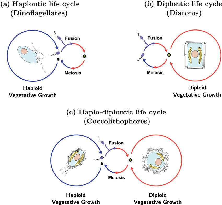
J. de Vries et al.: Haplo-diplontic life cycle expands coccolithophore niche                                                                    1167

Table 2. Taxonomic units included in HOLP index.

  Heterococcolithophores           Holococcolithophores
  C. mediterranea                  C. mediterranea HOL
  S. pulchra                       S. pulchra HOL
  S. protrudens
  S. bannockii                     S. bannockii HOL
  S. nana                          S. nana HOL
  S. arethusae                     S. arethusae HOL                            Figure 3. Hypervolume metrics utilized in this study: (a) union,
  S. nodosa                        H. cornifera                                (b) intersection, (c) unique fraction A, (d) Jaccard similarity metric,
  S. histrica                      S. histrica HOL                             (e) niche expansion, and (f) Sørensen–Dice similarity.
  S. molischii                     S. molischii HOL
  S. anthos                        S. anthos HOL
  S. strigilis                     S. strigilis HOL                            concentrations of phosphate, DIN, and silicate of the BATS
  S. halldalii                     S. halldalii HOL                            and Mediterranean data sets.
  S. marginiporata                 S. marginiporata HOL
  S. apsteinii                     S. apsteinii HOL                            2.5   Niche overlap and niche expansion
  P. japonica                      P. japonica HOL
  H. carteri                       H. carteri HOL                              Distribution patterns of phytoplankton are influenced by
  H. wallichii                     H. wallichii HOL                            multiple environmental drivers. These environmental drivers
  H. pavimentum                    Helicosphaera HOL dalmaticus type
                                                                               form a n-dimensional hyperspace within which hypervol-
  A. quattrospina                  A. quattrospina HOL
  A. robusta                       S. quadridentata                            umes can be defined based on where the phytoplankton oc-
  R. clavigera                                                                 cur. This hypervolume is considered to be the species niche
  R. xiphos                                                                    (Hutchinson, 1957) and allows niche comparisons between
  C. aculeata                      C. heimdaliae                               multiple phytoplankton – in this instance the two life cycle
  C. leptoporus                    C. leptoporus HOL                           phases of coccolithophores.
  C. pelagicus                     C. pelagicus HOL                               Although processing hypervolumes is challenging due to
  C. quadriperforatus              C. quadriperforatus HOL                     their high dimensionality, methods described by Blonder
  C. sphaeroidea                   C. sphaeroidea HOL
                                                                               et al. (2014) allow hypervolume quantification and compari-
  P. arctica                       P. arctica HOL
  P. sagittifera                   P. sagittifera HOL                          son (for further discussion see Blonder, 2018 and Mammola,
  P. borealis                      P. borealis HOL                             2019). Using this strategy we determine the niche overlap of
  B. virgulosa                     B. virgulosa HOL                            heterococcolithophores and holococcolithophores in hyper-
                                                                               space using the Sørensen–Dice and Jaccard similarity met-
Taxonomic units included in HOLP index. Note that in some instances multiple
heterococcolithophores are associated with single holococcolithophores (e.g.   rics.
S. pulchra and S. protrudens are both associated with S. pulchra HOL).            We furthermore calculate the “niche expansion” of the
                                                                               haplo-diplontic life cycle strategy, which we define here as
                                                                               the non-overlapping region of either phase within hyper-
the abundance and environmental parameters as a function of                    space. In other words,
latitude and depth. While for the Mediterranean data set the
variables were plotted as a function of the first two axes of a                            |A| − |A ∩ B|
                                                                               NE(A) =                   ,                                        (2)
PCA, which included temperature; salinity; day length; and                                    |A ∪ B|
concentrations of phosphate, DIN, and silicate. Two different
strategies were used to visualize the AMT and Mediterranean                    where NE(A) is a niche expansion of A, A is hypervolume
data sets, as the AMT data set is spatial and the Mediter-                     A, B is hypervolume B, ∩ is the intersection between two
ranean data set is temporal. The MBA interpolation was per-                    hypervolumes, and ∪ is a union between two hypervolumes.
formed with the “mba.surf” function from the “MBA” R                              The niche metrics utilized in this study are illustrated in
package (Finley et al., 2017), and the PCA was performed                       Fig. 3. Although we visualize the niche of each species us-
with the “dudi” function of the “ade4” package (Dray and                       ing contours, in reality the niche metrics are calculated based
Dufour, 2007). Cook’s distances were calculated using the                      on random points sampled from the inferred hypervolumes
“lm” and “cooks.distance” functions provided in the “stats”                    (Blonder et al., 2014).
R package (R Core Team, 2019).                                                    We calculated the Jaccard and Sørensen–Dice similar-
                                                                               ity metrics and niche expansion for the AMT, BATS, and
2.4    Seasonality                                                             Mediterranean Sea data sets. For the AMT data set, DIN
                                                                               showed high Pearson correlation to silicate (ρ = 0.95, p <
To investigate seasonality we compared monthly hetero-                         0.001) and phosphate (ρ = 0.90, p < 0.001). We thus only
coccolithophore and holococcolithophore abundance data to                      considered temperature, salinity, and the concentration of
temporal variations of temperature; salinity; day length; and                  DIN in this region. Although no such correlation was ob-

https://doi.org/10.5194/bg-18-1161-2021                                                                  Biogeosciences, 18, 1161–1184, 2021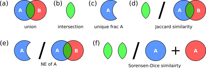
1168                                             J. de Vries et al.: Haplo-diplontic life cycle expands coccolithophore niche

served for the Mediterranean data set, and weaker but sig-        ≈ 9.78 × 10⁴ cells L−1 respectively), and March–May in the
nificant relationships were observed in the BATS stations         Pacific Ocean (≈ 4.96 × 10⁴ cells L−1 ).
(ρ = 0.74, p < 0.001 for silicate and ρ = 0.84, p < 0.001            The regions and periods with the highest mean hetero-
for phosphate), to make the niche metrics comparable in           coccolithophore abundance differ from the regions and peri-
all regions the silicate and phosphate concentrations of the      ods with the highest maximum heterococcolithophore abun-
Mediterranean and BATS data sets were also excluded.              dance. For example, the highest mean abundance is ob-
   It is likely, however, that silicate and phosphate, as well    served in the Indian Ocean during March–May (≈ 1.13×10⁵
as other parameters (such as irradiance, turbulence and car-      (±2.97 × 10⁴ ) cells L−1 ), which is higher than the highest
bonate chemistry), influence the niche of coccolithophores        mean abundance in the Southern Ocean observed during
and thus the metrics calculated. Besides the influence of en-     March–May (≈ 1.17 × 10⁵ (±2.88 × 10⁴ ) cells L−1 ) and in
vironmental parameter choice, results of the niche analysis       the Arctic Circle during June–August (≈ 5.83×10⁴ (±2.97×
will depend on what is considered a paired species. Although      104 ) cells L−1 ).
we use up-to-date definitions from Frada et al. (2018), these        Although holococcolithophores show low abundances in
definitions are likely to change in the future. Finally, cryp-    the high latitudes of the Southern Hemisphere, highest
tic speciation (Geisen et al., 2002) and subsequently the pair-   maximum holococcolithophore abundances are observed in
ing of multiple haploid holococcolith (HOL) phases to single      the Arctic circle (> 66◦ N) during June–August (≈ 2.23 ×
diploid heterococcolith (HET) phases and vice versa compli-       105 cells L−1 ). High maximum abundances are additionally
cate results.                                                     observed in the Mediterranean Sea (September–November)
   The environmental data were normalized using z scores          (≈ 1.27 × 10⁵ cells L−1 ).
prior to analysis. Niche overlap and niche expansion were            The lowest maximum holococcolithophore abundance is
calculated only for species for which both life cycle phases      observed in the Pacific Ocean during June–August (4.45 ×
were observed. In addition to calculating the niche expansion     102 cells L−1 ) and in the Arctic Circle during September–
for individual species, we calculated an average niche expan-     November (1.12 × 10³ cells L−1 ).
sion by taking the mean NE values of all individual species          On average, the Mediterranean Sea has the highest
for both the haploid and diploid coccolithophore life cycle       mean holococcolithophore abundance (between ≈ 2.21 ×
phases.                                                           103 and 9.42 × 10³ cells L−1 ), followed by the Indian
   We used the “hypervolume” R package (Blonder and Har-          Ocean (≈ 1.41×10³ –4.80×10³ cells L−1 ). The lowest mean
ris, 2018) to conduct our niche overlap and niche expan-          abundances are observed in the Pacific Ocean (4.9 ×
sion analysis. Gaussian kernel density estimation (R function     101 (±9.70 × 101 ), Arctic Circle (September–November;
“hypervolume_gaussian”) was used to construct the hyper-          2.55 × 10² (±2.71 × 10² ), and Southern Ocean (December–
volume, the overlap metrics were calculated with the “hy-         February; ≈ 3.24 × 10² (±2.06 × 10² ) cells L−1 ).
pervolume_overlap_statistics” R function, and the volume             Depending on the season, holococcolithophore contri-
and intersection of hyper volumes were calculated using the       bution to total coccolithophore abundance varies glob-
“get_volume” R function.                                          ally between 1.67 % (±0.37 %) in December–February and
                                                                  16.16 % (±1.68 %) in June–August, with the highest con-
                                                                  tribution observed in the Mediterranean Sea in June–August
                                                                  (31.38 % ± 2.93 %) (Table 3). On an regional scale outside of
3     Results                                                     the Mediterranean Sea, holococcolithophores contribute less
                                                                  than 8 % to the total coccolithophore abundances. However,
3.1    Biogeography of coccolithophores                           the contribution of holococcolithophores to paired species is
                                                                  higher than when all heterococcolithophore and holococcol-
Within our compilation, heterococcolithophores showed             ithophores are considered (Table 4), with a HOLP index be-
global distribution, while holococcolithophores were notice-      tween 5.65 % (±1.71 %) and 27.41 (±2.67 %) globally de-
ably absent at the ALOHA station in Hawaii and (with some         pending on season. The lowest HOLP indices were observed
exceptions) > 50◦ S in the Southern Ocean (Fig. 4 and Ta-         in the Atlantic Ocean in September–November (0.59 ± 0.81)
ble 3).                                                           and December–February (0.47 ± 0.65 %), and in the South-
   The highest maximum abundances of heterococcol-                ern Ocean in December–February (0.61±0.58 %). The high-
ithophores are observed at high latitudes within the Arc-         est HOLP index was observed in the Mediterranean Sea in
tic Circle (> 66◦ N) (≈ 4.37 × 10⁶ cells L−1 for June–            June–August (39.03 ± 3.23 %).
August) and the Southern Ocean (> 40 and < 65◦ S) (≈
1.64 × 10⁶ cells L−1 for December–February). Generally,
                                                                  3.2   Vertical distribution
maximum abundances above 1 × 10⁵ cells L−1 were ob-
served, except between September–November in the Indian
Ocean (≈ 3.33 × 10⁴ cells L−1 ), September–November and           In the global data set, heterococcolithophore abundance is
December–February in the Atlantic Ocean (≈ 5.40×10⁴ and           evenly distributed with depth, while holococcolithophore

Biogeosciences, 18, 1161–1184, 2021                                                 https://doi.org/10.5194/bg-18-1161-2021
J. de Vries et al.: Haplo-diplontic life cycle expands coccolithophore niche 1169
Table 3. Global heterococcolithophore and holococcolithophore abundance.
Location Season Phase Mean (± ci) (cells L−1 ) Max (cells L−1 ) Contribution (± ci)(%) n
Global Mar–May HET 4.57 × 10⁴ (± 4.72 × 10³ ) 4.93 × 10⁵ 93.72 (± 0.98) 585
HOL 2.00 × 10³ (± 5.42 × 10² ) 8.72 × 10⁴ 5.05 (± 0.93) 585
Jun–Aug HET 4.36 × 10⁴ (± 1.56 × 10⁴ ) 4.37 × 10⁶ 82.53 (± 1.68) 739
HOL 4.64 × 10³ (± 1.03 × 10³ ) 2.23 × 10⁵ 16.16 (± 1.68) 739
Sep–Nov HET 1.75 × 10⁴ (± 3.09 × 10³ ) 3.53 × 10⁵ 91.46 (± 1.61) 438
HOL 1.74 × 10³ (± 8.27 × 10² ) 1.27 × 10⁵ 7.11 (± 1.59) 438
Dec–Feb HET 9.32 × 10⁴ (± 8.99 × 10³ ) 1.64 × 10⁶ 95.37 (± 0.66) 772
HOL 1.78 × 10³ (± 4.76 × 10² ) 1.18 × 10⁵ 1.67 (± 0.37) 772
Arctic Circle Jun–Aug HET 5.83 × 10⁴ (± 4.53 × 10⁴ ) 4.37 × 10⁶ 95.87 (± 2.12) 213
HOL 1.83 × 10³ (± 2.18 × 10³ ) 2.23 × 10⁵ 3.71 (± 2.02) 213
Sep–Nov HET 3.41 × 10⁴ (± 2.51 × 10⁴ ) 1.29 × 10⁵ 94.79 (± 5.53) 11
HOL 2.55 × 10² (± 2.71 × 10² ) 1.12 × 10³ 5.21 (± 5.53) 11
East China Sea Sep–Nov HET 2.99 × 10⁴ (± 1.30 × 10⁴ ) 2.39 × 10⁵ 96.48 (± 3.97) 51
HOL 9.06 × 10² (± 7.98 × 10² ) 1.47 × 10⁴ 3.52 (± 3.97) 51
Indian Ocean Mar–May HET 1.13 × 10⁵ (± 2.97 × 10⁴ ) 2.18 × 10⁵ 96.88 (± 1.3) 33
HOL 1.41 × 10³ (± 7.85 × 10² ) 1.10 × 10⁴ 2.35 (± 1.31) 33
Jun–Aug HET 2.40 × 10⁴ (± 7.38 × 10³ ) 1.11 × 10⁵ 90.11 (± 3.53) 53
HOL 6.57 × 10² (± 2.67 × 10² ) 3.43 × 10³ 3.68 (± 2.09) 53
Sep–Nov HET 7.03 × 10³ (± 1.50 × 10³ ) 3.33 × 10⁴ 89.33 (± 3.78) 89
HOL 2.87 × 10² (± 2.00 × 10² ) 5.63 × 10³ 5.57 (± 3.49) 89
Dec–Feb HET 2.00 × 10⁵ (± 1.71 × 10³ ) 2.27 × 10⁵ 96.56 (± 0.64) 102
HOL 4.80 × 10³ (± 1.27 × 10³ ) 3.10 × 10⁴ 2.3 (± 0.6) 102
Mediterranean Sea Mar–May HET 2.80 × 10⁴ (± 4.90 × 10³ ) 2.11 × 10⁵ 88.88 (± 3.19) 146
HOL 3.76 × 10³ (± 1.83 × 10³ ) 8.72 × 10⁴ 10.55 (± 3.06) 146
Jun–Aug HET 1.21 × 10⁴ (± 1.95 × 10³ ) 1.00 × 10⁵ 68.42 (± 2.92) 290
HOL 9.42 × 10³ (± 1.94 × 10³ ) 1.02 × 10⁵ 31.38 (± 2.93) 290
Sep–Nov HET 1.70 × 10⁴ (± 4.38 × 10³ ) 3.53 × 10⁵ 89.11 (± 2.89) 195
HOL 3.10 × 10³ (± 1.82 × 10³ ) 1.27 × 10⁵ 10.2 (± 2.91) 195
Dec–Feb HET 4.23 × 10⁴ (± 1.18 × 10⁴ ) 3.96 × 10⁵ 96.78 (± 1.11) 125
HOL 2.21 × 10³ (± 2.33 × 10³ ) 1.18 × 10⁵ 1.96 (± 0.92) 125
Atlantic Ocean Mar–May HET 4.20 × 10⁴ (± 5.68 × 10³ ) 1.83 × 10⁵ 96.78 (± 0.87) 174
HOL 1.20 × 10³ (± 5.36 × 10² ) 2.76 × 10⁴ 1.88 (± 0.6) 174
Jun–Aug HET 1.51 × 10⁵ (± 6.84 × 10⁴ ) 1.55 × 10⁶ 93.6 (± 2.07) 86
HOL 1.70 × 10³ (± 8.96 × 10² ) 2.29 × 10⁴ 3.89 (± 1.6) 86
Sep–Nov HET 1.48 × 10⁴ (± 4.56 × 10³ ) 5.40 × 10⁴ 96.76 (± 1.34) 30
HOL 3.77 × 10² (± 1.54 × 10² ) 1.39 × 10³ 2.59 (± 1.22) 30
Dec–Feb HET 2.50 × 10⁴ (± 9.70 × 10³ ) 9.78 × 10⁴ 94.23 (± 3.09) 29
HOL 3.38 × 10² (± 1.55 × 10² ) 1.64 × 10³ 1.81 (± 1.26) 29
Pacific Ocean Mar–May HET 1.43 × 10⁴ (± 6.24 × 10³ ) 4.96 × 10⁴ 92.33 (± 6.63) 25
HOL 4.50 × 10³ (± 4.56 × 10³ ) 3.98 × 10⁴ 7.55 (± 6.64) 25
Jun–Aug HET 1.96 × 10⁴ (± 3.17 × 10⁴ ) 1.48 × 10⁵ 98.12 (± 1.64) 9
HOL 4.90 × 101 (± 9.70 × 101 ) 4.45 × 10² 0.03 (± 0.07) 9
Dec–Feb HET 2.00 × 10⁴ (± 1.32 × 10⁴ ) 1.64 × 10⁵ 94.85 (± 4.02) 28
HOL 8.65 × 10² (± 1.20 × 10³ ) 1.70 × 10⁴ 0.89 (± 0.75) 28
Southern Ocean Mar–May HET 1.17 × 10⁵ (± 2.88 × 10⁴ ) 4.93 × 10⁵ 98.19 (± 0.88) 50
HOL 9.10 × 10² (± 6.55 × 10² ) 1.60 × 10⁴ 1.36 (± 0.87) 50
Dec–Feb HET 9.10 × 10⁴ (± 1.66 × 10⁴ ) 1.64 × 10⁶ 99.05 (± 0.7) 332
HOL 3.24 × 10² (± 2.06 × 10² ) 2.67 × 10⁴ 0.95 (± 0.7) 332
Values in parentheses are 95 % confidence intervals.
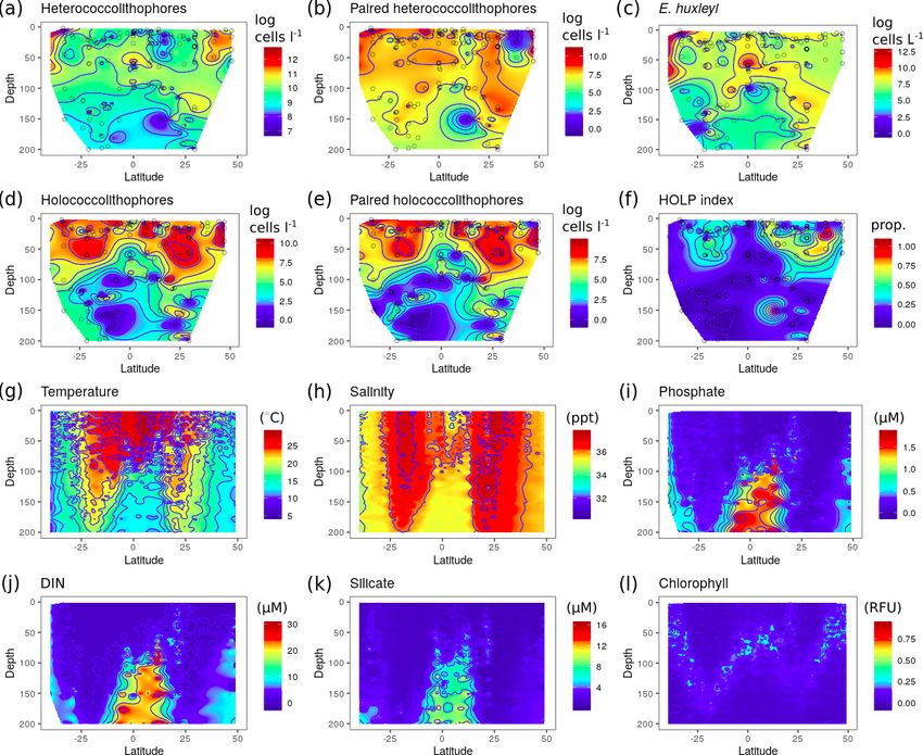
https://doi.org/10.5194/bg-18-1161-2021 Biogeosciences, 18, 1161–1184, 20211170 J. de Vries et al.: Haplo-diplontic life cycle expands coccolithophore niche Figure 4. (a–b) Global coccolithophore distribution and (c–h) latitudinal coccolithophore distribution: (a) Heterococcolithophores, (b) Holo- coccolithophores, (c) Heterococcolithophores, (d) E. huxleyi, (e) paired heterococcolithophores, (f) holococcolithophores, (g) paired holo- coccolithophores, and (h) HOLP index. For the latitudinal plots, the light shading is log-transformed distribution. abundance is highest in the top 50 m of the water column aster formosus, Florisphaera profunda, Calciopappus cau- (Fig. 5). datus, and Oolithotus antillarum. However, although paired For holococcolithophores the vertical distribution pattern heterococcolithophores only contributed ≈ 5.7 % to total het- is mainly driven by paired holococcolithophore species, erococcolithophore abundance, the depth distribution trends which constituted ≈ 62.2 % of the total coccolithophore of paired and total heterococcolithophores species were sim- abundance. Two currently unpaired holococcolithophores ilar. also contribute to the depth distribution trend with Hella- dosphaera cornifera (for which the association has to be 3.3 Environmental drivers of niche partitioning further confirmed), constituting ≈ 8.1 % of total holococcol- ithophore abundance, and Corisphaera gracilis (for which To further understand the distribution patterns observed on no pair has been described), constituting ≈ 3.6 % of total a global basis and within the water column we investigated holococcolithophore abundance. Subsequently paired holo- the environmental drivers of heterococcolithophore and holo- coccolithophore abundances broadly followed the same pat- coccolithophore abundance in the Atlantic Ocean (with the terns observed when all holococcolithophores were consid- AMT data set) and the Mediterranean Sea. For the Atlantic ered. Ocean data set, the environmental drivers were considered In comparison to holococcolithophores, depth distribution in the context of their distribution within the water column, of heterococcolithophores was driven by unpaired species, whereas for the Mediterranean the environmental drivers in particular E. huxleyi, which constituted ≈ 59.2 % of to- were considered within PCA “niche space”. These observed tal heterococcolithophore abundance, but was also driven by patterns were then further corroborated through Spearman the presence of unpaired deep-water species such as Ophi- analysis. Biogeosciences, 18, 1161–1184, 2021 https://doi.org/10.5194/bg-18-1161-2021
J. de Vries et al.: Haplo-diplontic life cycle expands coccolithophore niche                                                        1171

Figure 5. Global depth distribution of heterococcolithophores and holococcolithophores: (a–d) total paired and unpaired heterococcol-
ithophore and holococcolithophore abundance and (e–f) individual species abundances. Heterococcolithophores are plotted in red, and holo-
coccolithophores are plotted in blue. Only the most abundant coccolithophore species are plotted individually. Error bars are the standard
error.

3.3.1   Atlantic Ocean                                                    This suggests that heterococcolithophores might be better
                                                                       adapted to exploit such conditions. Although differences in
In the Atlantic Ocean both heterococcolithophores and holo-            sinking rates, which are conceivably higher in the more heav-
coccolithophores have their highest abundances in the top              ily calcified heterococcolithophores, could also factor into
50 m of the water column (Fig. 6). However, a noticeable               the difference in depth distribution between the two life cycle
difference between heterococcolithophore and holococcol-               phases.
ithophore distribution (Fig. 6a and d respectively) is the ab-            The distribution of heterococcolithophores (Fig. 6a) is
sence of holococcolithophores below the deep chlorophyll               primarily driven by E. huxleyi (Fig. 6c), which constitutes
maximum (DCM) (Fig. 6l). The DCM tends to occur at 1 %–                ≈ 30 % of total heterococcolithophore abundance in the data
10 % irradiance levels and is closely linked to the nutricline         set. When only paired heterococcolithophore species were
and thermocline (Poulton et al., 2006). The difference in              considered (Fig. 6b), a more even distribution in subtropical
depth distribution between heterococcolithophores and holo-            and tropical regions is observed. Holococcolithophores and
coccolithophores and the absence of holococcolithophores               paired holococcolithophores showed roughly similar distri-
below the DCM may therefore be influenced by a combi-                  bution patterns (Fig. 6d and e).
nation of light limitation, high nutrient concentrations, cold            Within the upper water column, heterococcolithophores
water temperatures at depth, or other factors not addressed in         showed the highest abundance at higher latitudes (> 35◦ N
this study.

https://doi.org/10.5194/bg-18-1161-2021                                                         Biogeosciences, 18, 1161–1184, 2021
1172 J. de Vries et al.: Haplo-diplontic life cycle expands coccolithophore niche Figure 6. Depth distribution along AMT: (a) heterococcolithophore abundance, (b) paired heterococcolithophore abundance, (c) E. huxleyi abundance, (d) holococcolithophore abundance, (e) paired holococcolithophore abundance, (f) HOLP index, (g) temperature (◦ C), (h) salinity (ppt), (i) DIN (µM), (j) silicate (µM), (k) silicate, and (l) chlorophyll. Species abundances are plotted on log scale. and > 30◦ S), which is associated with a shallow mixed layer, On the contrary, heterococcolithophores are only signifi- lower salinity, and lower temperature, as well as increasing cantly and negatively correlated with depth and phosphate. silicate concentrations in the Southern Hemisphere. Holo- While for paired heterococcolithophores significant negative coccolithophores meanwhile showed the highest abundances correlations were observed with depth and silicate. at both high latitudes and in the Atlantic subtropical gyres. Thus heterococcolithophore and holococcolithophore The HOLP index (Fig. 6f) was highest within the Atlantic abundance in the Atlantic Ocean seems primarily driven by subtropical gyres, with a higher proportion of holococcol- the depth of the DCM both in terms of vertical and latitudi- ithophores in the northern subtropical gyre, which is associ- nal distribution. The highest abundances of both heterococ- ated with a shallower DCM relative to the southern subtrop- colithophores and holococcolithophores are observed above ical gyre. This shallowing of the DCM on the AMT is, how- the DCM, and heterococcolithophores are present below the ever, likely a seasonal signal as described by Poulton et al. DCM while holococcolithophores are not. In terms of lati- (2006) and Poulton et al. (2017). tude, the highest abundances of heterococcolithophores cor- Spearman correlations (Table 6) suggests holococcol- respond to the shallow DCM depth that occurs in higher- ithophores are significantly (p < 0.05) negatively correlated latitude regions, and the highest abundances of holococ- to phosphate, DIN, silicate, and depth and significantly posi- colithophores occur in subtropical regions with deep DCM tively correlated to temperature and salinity. Paired holococ- depths. colithophores and the HOLP index showed the same correla- tion trends as holococcolithophores. Biogeosciences, 18, 1161–1184, 2021 https://doi.org/10.5194/bg-18-1161-2021
J. de Vries et al.: Haplo-diplontic life cycle expands coccolithophore niche                                                              1173

Table 4. Global HOLP index.                                                     ues (i.e. the right quadrants of Fig. 7b), which correspond to
                                                                                high temperatures and long day lengths and low salinity and
    Location                   Season          Mean                      n      concentrations of DIN, silicate, and phosphate.
    Global                     Mar–May         17.33 (± 2.55)         332          The pattern observed in the PCA niche space should be
                               Jun–Aug         27.41 (± 2.67)         484       interpreted with some caution because only a portion of the
                               Sep–Nov         18.29 (± 3.84)         241       variance is captured (53 %) and the use of interpolation intro-
                               Dec–Feb         5.65 (± 1.71)          257       duces additional uncertainties. Besides, the structure of the
                                                                                PCA depends highly on the number and type of variables in-
    Arctic Circle              Jun–Aug         13.01 (± 5.44)         107
                                                                                cluded (Figs. S2–S4 in the Supplement), particularly when
    East China Sea             Sep–Nov         17.06 (± 8.25)           40      time is considered. However, the patterns presented in the
    Indian Ocean               Mar-May         4.7 (± 4.49)             16      PCA are also apparent in the Spearman correlations (see Ta-
                               Jun–Aug         15.78 (± 9.55)           26      ble 6), which suggests that the PCA plots are a qualitatively
                               Sep–Nov         26.42 (± 12.05)          51      good representation of the data.
                                                                                   The Spearman correlations indicate that heterococcol-
    Mediterranean Sea          Mar–May         25.68 (± 4.28)         140
                                                                                ithophores are significantly negatively correlated to tempera-
                               Jun–Aug         39.03 (± 3.23)         285
                               Sep–Nov         16.84 (± 4.11)         123       ture and day length and significantly positively correlated to
                               Dec–Feb         7.23 (± 2.97)           97       phosphate, DIN, silicate, and salinity. For paired heterococ-
                                                                                colithophore species the only significant correlation observed
    Atlantic Ocean             Mar–May         10.05 (± 3.04)         116       was a positive correlation with silicate.
                               Jun–Aug         6.13 (± 4.91)           48
                                                                                   Holococcolithophores showed the opposite pattern to hete-
                               Sep–Nov         0.59 (± 0.81)           12
                                                                                rococcolithophores and are significantly positively correlated
                               Dec–Feb         0.47 (± 0.65)           19
                                                                                to day length and temperature and significantly negatively
    Pacific Ocean              Mar–May         38.2 (± 20.58)           15      correlated to salinity, DIN, silicate, and phosphate. Paired
                               Dec–Feb         34.85 (± 17.08)          12      holococcolithophores and the HOLP index showed signifi-
                               Dec–Feb         0.61 (± 0.58)            40      cant positive correlation to temperature and day length, but
  Mean HOLP indices grouped by season and location. Values in parentheses are   no significant correlations with the other environmental vari-
  the 95 % confidence interval.                                                 ables were observed.

Table 5. PCA loadings of the Mediterranean Sea data set.                        3.3.3   General environmental trends

                    Variable              PC1         PC2                       Our statistical analysis shows that in both the Mediterranean
                                                                                Sea and Atlantic Ocean holococcolithophores are generally
                    Temperature         1.57       −0.75
                                                                                found in low-nutrient and warm environments and high light
                    Salinity           −1.25        1.23
                    DIN                −0.42       −1.04
                                                                                availability. However, an opposite trend was observed be-
                    Silicate           −0.98       −1.27                        tween the Atlantic Ocean and Mediterranean Sea in terms
                    Phosphate          −0.81       −0.89                        of correlation to salinity, with holococcolithophores posi-
                    Day length          1.17        0.27                        tively correlated to salinity in the Atlantic Ocean and neg-
                                                                                atively correlated to salinity in the Mediterranean Sea. This
                  The first two axis of the PCA captured
                  53.94 % of variance. Data are from Cerino                     difference in correlation to salinity may be explained by the
                  et al. (2017) and Godrijan et al. (2018).                     different drivers of salinity in both regions. In the Atlantic
                                                                                Ocean, low salinity occurs at high latitudes, while high salin-
                                                                                ity corresponds to mid-ocean gyres due to higher evapora-
3.3.2   Mediterranean Sea                                                       tion in tropical and subtropical regions. In contrast, at the
                                                                                coastal site in the Mediterranean Sea, low salinity is strictly
For the Mediterranean Sea long-term time series, niche sep-                     related to direct freshwater input and associated nutrients. As
aration of heterococcolithophores and holococcolithophores                      such salinity may be simply correlated to other environmen-
within the PCA niche space (Fig. 7) is primarily driven by                      tal drivers, rather than be a driver itself.
principal component 1 (PC1), which is positively associated                        In the Mediterranean Sea and the Atlantic Ocean signifi-
with temperature and day length and negatively associated                       cant negative correlations were observed between holococ-
with salinity, DIN, silicate, and phosphate (see Table 7). Het-                 colithophores and silicate. Although this correlation could
erococcolithophores are most abundant at low PC1 values                         be in part due to strong correlation between DIN and sili-
(i.e. the left quadrants of Fig. 7a), which correspond to low                   cate (ρ = 0.95) observed in the Atlantic Ocean, the reason
temperatures and short day lengths and high salinity and con-                   for this is less clear in the Mediterranean Sea as no such cor-
centrations of DIN, silicate, and phosphate (see Table 5).                      relation is observed. A physiological reason for the negative
Holococcolithophores are most abundant at high PC1 val-                         correlation to silicate could be different silicate requirements

https://doi.org/10.5194/bg-18-1161-2021                                                                Biogeosciences, 18, 1161–1184, 2021
1174 J. de Vries et al.: Haplo-diplontic life cycle expands coccolithophore niche
Table 6. Spearman correlations for the AMT data set.
Phase Temp Sal PO4 NOx Depth Si
HET −0.095 −0.085 −0.298∗ −0.095 −0.323∗∗∗ −0.139
HET.P 0.13 0.136 −0.069 −0.092 −0.384∗∗∗ −0.295∗∗
HOL 0.339∗∗∗ 0.224∗∗ −0.327∗ −0.609∗∗∗ −0.584∗∗∗ −0.52∗∗∗
HOL.P 0.327∗∗∗ 0.233∗∗ −0.289∗ −0.55∗∗∗ −0.58∗∗∗ −0.502∗∗∗
HOLP 0.31∗∗∗ 0.236∗∗ −0.506∗∗∗ −0.587∗∗∗ −0.472∗∗∗ −0.469∗∗∗
∗∗∗ p < 0.001. ∗∗ p < 0.01. ∗ p < 0.05. Significant correlations are highlighted in bold. Data were acquired from
Poulton et al. (2017). The following abbreviations are used within this table: HET stands for heterococcolithophores,
HET.P stands for paired heterococcolithophores, HOL stands for holococcolithophores, HOL.P stands for paired
holococcolithophores, and HOLP stands for the HOLP index.
Figure 7. Principal component analysis (PCA) of the RV-001 and LTER1 stations in the Mediterranean Sea. Abundance and environmental
values were projected on the PCA post hoc and then interpolated: (a) heterococcolithophore abundance, (b) holococcolithophore abundance,
(c) salinity, (d) temperature, (e) depth, (f) phosphate, (g) DIN, and (h) silicate. Data were acquired from Cerino et al. (2017) and Godrijan
et al. (2018).
among different coccolithophore species. Durak et al. (2016) ith life cycle phases of C. coccolithus and C. leptoporus do
for instance found evidence of silicate requirement for the not require silicate (Langer et al., 2021).
heterococcolith life cycle phases of S. apsteinii, C. coccol- Statistically significant correlations were the same when
ithus, and C. leptoporus but not for E. huxleyi or G. oceanica. all holococcolithophores, paired holococcolithophores, or
Follow-up experiments have furthermore found holococcol- the HOLP index was considered at both locations; however,
Biogeosciences, 18, 1161–1184, 2021 https://doi.org/10.5194/bg-18-1161-2021You can also read