Air-sea exchange of acetone, acetaldehyde, DMS and isoprene at a UK coastal site - Recent
←
→
Page content transcription
If your browser does not render page correctly, please read the page content below
Atmos. Chem. Phys., 21, 10111–10132, 2021
https://doi.org/10.5194/acp-21-10111-2021
© Author(s) 2021. This work is distributed under
the Creative Commons Attribution 4.0 License.

Air–sea exchange of acetone, acetaldehyde, DMS and
isoprene at a UK coastal site
Daniel P. Phillips1,2 , Frances E. Hopkins1 , Thomas G. Bell1 , Peter S. Liss2 , Philip D. Nightingale1,2,3 ,
Claire E. Reeves2 , Charel Wohl1,2 , and Mingxi Yang1
1 Plymouth  Marine Laboratory, Plymouth, PL1 3DH, UK
2 Centre for Ocean and Atmospheric Sciences, School of Environmental Sciences,
University of East Anglia, Norwich, NR4 7TJ, UK
3 Sustainable Agriculture Systems, Rothamsted Research, North Wyke, EX20 2SB, UK

Correspondence: Daniel P. Phillips (dph@pml.ac.uk) and Mingxi Yang (miya@pml.ac.uk)

Received: 4 February 2021 – Discussion started: 2 March 2021
Revised: 21 May 2021 – Accepted: 2 June 2021 – Published: 6 July 2021

Abstract. Volatile organic compounds (VOCs) are ubiqui-           greater deposition fluxes of acetone and acetaldehyde within
tous in the atmosphere and are important for atmospheric          the Plymouth Sound were likely to a large degree driven by
chemistry. Large uncertainties remain in the role of the ocean    higher atmospheric concentrations from the terrestrial wind
in the atmospheric VOC budget because of poorly con-              sector. The reduced DMS emission from the Plymouth Sound
strained marine sources and sinks. There are very few direct      was caused by a combination of lower wind speed and likely
measurements of air–sea VOC fluxes near the coast, where          lower dissolved concentrations as a result of the estuarine in-
natural marine emissions could influence coastal air quality      fluence (i.e. dilution).
(i.e. ozone, aerosols) and terrestrial gaseous emissions could       In addition, we measured the near-surface seawater con-
be taken up by the coastal seas.                                  centrations of acetone, acetaldehyde, DMS and isoprene
   To address this, we present air–sea flux measurements          from a marine station 6 km offshore. Comparisons are made
of acetone, acetaldehyde and dimethylsulfide (DMS) at the         between EC fluxes from the open-water and bulk air–sea
coastal Penlee Point Atmospheric Observatory (PPAO) in the        VOC fluxes calculated using air and water concentrations
south-west UK during the spring (April–May 2018). Fluxes          with a two-layer (TL) model of gas transfer. The calcu-
of these gases were measured simultaneously by eddy covari-       lated TL fluxes agree with the EC measurements with re-
ance (EC) using a proton-transfer-reaction quadrupole mass        spect to the directions and magnitudes of fluxes, implying
spectrometer. Comparisons are made between two wind sec-          that any recently proposed surface emissions of acetone and
tors representative of different air–water exchange regimes:      acetaldehyde would be within the propagated uncertainty of
the open-water sector facing the North Atlantic Ocean and         2.6 µmol m−2 d−1 . The computed transfer velocities of DMS,
the terrestrially influenced Plymouth Sound fed by two estu-      acetone and acetaldehyde from the EC fluxes and air and wa-
aries.                                                            ter concentrations are largely consistent with previous trans-
   Mean EC (± 1 standard error) fluxes of acetone, ac-            fer velocity estimates from the open ocean. This suggests that
etaldehyde and DMS from the open-water wind sector were           wind, rather than bottom-driven turbulence and current ve-
−8.0 ± 0.8, −1.6 ± 1.4 and 4.7 ± 0.6 µmol m−2 d−1 respec-         locity, is the main driver for gas exchange within the open-
tively (“−” sign indicates net air-to-sea deposition). These      water sector at PPAO (depth of ∼ 20 m).
measurements are generally comparable (same order of
magnitude) to previous measurements in the eastern North
Atlantic Ocean at the same latitude. In comparison, the
Plymouth Sound wind sector showed respective fluxes of
−12.9 ± 1.4, −4.5 ± 1.7 and 1.8 ± 0.8 µmol m−2 d−1 . The

Published by Copernicus Publications on behalf of the European Geosciences Union.
10112                                    D. P. Phillips et al.: Air–sea exchange of acetone, acetaldehyde, DMS and isoprene

1   Introduction                                                   Loreto, 2017). Oceanic sources of isoprene are important for
                                                                   the remote marine atmosphere (Lewis et al., 2001; Arnold et
Volatile organic compounds (VOCs) are ubiquitous in the at-        al., 2009; Booge et al., 2016) where transport from terrestrial
mosphere and play an important role in atmospheric chem-           sources is negligible due to isoprene’s very short atmospheric
istry and carbon cycling in the biosphere (Heald et al.,           lifetime (∼ 30 min; Carslaw et al., 2000).
2008). Many VOCs can influence the oxidative capacity                 The main oceanic sink of most VOCs is biological
of the atmosphere by acting as a source or sink of atmo-           metabolism at varying rates (Dixon et al., 2014; Royer et al.,
spheric ozone (O3 ) and hydroxyl radicals (Atkinson, 2000;         2016; Halsey et al., 2017). Surface seawater concentrations
Lewis et al., 2005), thereby influencing local air quality. The    of acetone and acetaldehyde tend not to be very sensitive to-
lower volatility oxidation products, produced from reactions       wards their air–sea fluxes (Beale et al., 2015). Emission to
of some VOCs with atmospheric oxidants, can condense               the atmosphere is generally considered to be a small loss for
into particulates and form cloud condensation nuclei (CCN)         seawater DMS (Yang et al., 2013b) but a much larger loss
(Charlson et al., 1987; Blando and Turpin, 2000; Henze and         relatively for seawater isoprene (Booge et al., 2018).
Seinfeld, 2006), affecting the Earth’s radiative forcing and          There have been very few direct measurements of air–sea
climate.                                                           VOC fluxes with the eddy covariance (EC) technique (e.g.
   The terrestrial environment is the largest source of VOCs       Marandino et al., 2005; Yang et al., 2013c, 2014b; Kim et
to the atmosphere, with the emission dominated by isoprene         al., 2017). More often, the fluxes are estimated with the bulk
from plant foliage (Guenther et al., 2006). Terrestrial bio-       method using air and sea concentrations in a two-layer (TL)
logical processes also produce carbonyls, including ketones        model (e.g. Baker et al., 2000; Beale et al., 2013; Wohl et al.,
and aldehydes in varying amounts (Kesselmeier and Staudt,          2020). Most studies focus on open ocean air–sea exchange,
1999). Large uncertainties exist however with respect to the       while air–sea VOC flux measurements from the coast are es-
role that the ocean plays as a net source or sink of these gases   sentially non-existent (EC or bulk). Compared to the open
(Broadgate et al., 1997; Arnold et al., 2009; Millet et al.,       ocean, the coastal waters tend to be very dynamic biogeo-
2010; Fischer et al., 2012; Wang et al., 2019). This is due        chemically (Borges et al., 2005; Bauer et al., 2013) and phys-
to poorly quantified air–sea fluxes as well as uncertainties in    ically. For example, riverine runoffs carry nutrients and or-
the biogeochemical and physical processes that control them.       ganic carbon into the coastal seas, which could stimulate in-
   Acetone and acetaldehyde are carbonyl-based VOCs that           tense biological cycling (Cloern et al., 2014). Furthermore,
have been shown to make up to ∼ 57 % of the carbon mass            compared to the remote marine atmosphere, coastal air is af-
of all non-methane organic carbon compounds in remote ma-          fected by terrestrial emissions.
rine air over the North Atlantic Ocean (Lewis et al., 2005).          The air–sea gas transfer velocity can be derived by equat-
These VOCs have been detected in the surface ocean at con-         ing the EC flux with the bulk TL flux (e.g. Blomquist et
centrations of up to tens of nanomolar (nM) (Zhou and Mop-         al., 2010; Bell et al., 2013; Yang et al., 2013a, 2014a). Lim-
per, 1997; Williams et al., 2004), with known oceanic sources      ited studies have been undertaken to identify whether open-
including the photochemical degradation of dissolved or-           ocean-derived parameterisations of the transfer velocity are
ganic matter (DOM) in bulk seawater (Kieber et al., 1990;          applicable to coastal systems (Borges et al., 2004; Yang et al.,
Zhou and Mopper, 1997; Zhu and Kieber, 2018) and pos-              2019a). Turbulent processes (i.e. wave-breaking, tidal cur-
sibly autotrophic/heterotrophic biological processes (Halsey       rents, bottom driven turbulence) are expected to behave dif-
et al., 2017; Schlundt et al., 2017). The heterogeneous oxida-     ferently in these environments (Upstill-Goddard, 2006), with
tion of DOM at the sea surface has recently been identified        potential impacts on gas exchange.
as a source of carbonyl-containing VOCs (Zhou et al., 2014;           Here we present air–sea fluxes of acetone, acetaldehyde
Ciuraru et al., 2015); however the significance of this is cur-    and DMS determined using the EC technique at a coastal ob-
rently unknown.                                                    servatory in the south-west UK. Using seawater concentra-
   Dimethylsulfide (DMS) is a biogenic sulfur-containing           tions measured from a marine station 6 km offshore, we fur-
VOC that constitutes the majority of the organic sulfur in         ther compute the TL fluxes of these VOCs as well as the TL
the atmosphere (Andreae et al., 1985). It is produced in the       flux of isoprene. We compare our coastal flux measurements
surface ocean from the degradation of the algal osmolyte           with previous observations of open ocean fluxes as well as
dimethylsulfoniopropionate (Kiene et al., 2000) and subse-         global model estimates. From the EC fluxes and air and sea
quently emitted into the atmosphere. DMS is often the dom-         concentrations, we derive the gas transfer velocities of DMS,
inant source of sulfur in the marine atmosphere (Yang et al.,      acetone and acetaldehyde and compare them against previ-
2011b), and the oxidation products of DMS can act as CCN           ous observations from the open ocean.
(Charlson et al., 1987; Veres et al., 2020).
   Isoprene is an unsaturated terpene-based VOC that is pro-
duced in the ocean by a broad range of phytoplankton as a
secondary metabolic product (Moore et al., 1994; Shaw et
al., 2003; Exton et al., 2013; Booge et al., 2016; Dani and

Atmos. Chem. Phys., 21, 10111–10132, 2021                                          https://doi.org/10.5194/acp-21-10111-2021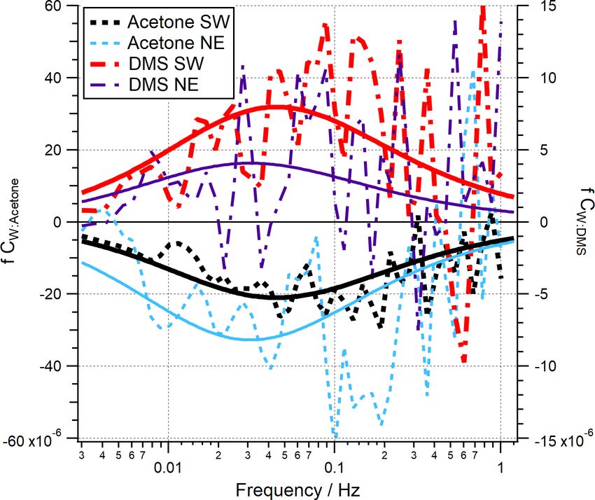
D. P. Phillips et al.: Air–sea exchange of acetone, acetaldehyde, DMS and isoprene                                           10113

                                                                     of a downwards-facing 90◦ union, mounted 30 cm below the
                                                                     anemometer, connected via a 10 m tube to a union tee up-
                                                                     stream of the air pump (UT1). All PPAO air sampling instru-
                                                                     ments (including the PTR-MS) subsampled ambient air from
                                                                     this union tee. A dry pump (Gast 1023 series) was used to
                                                                     draw ambient air into the observatory. The total flow rate was
                                                                     ∼ 13.5 L min−1 , as calculated from the continuously moni-
                                                                     tored flow of the pump (Bronkhurst EL-FLOW series) and
                                                                     the sum of independent flows of connected instruments. All
                                                                     unions and tubing before UT1 were 9.5 mm internal diameter
                                                                     (ID).
                                                                        Downstream of UT1 (i.e. closer to the instruments) was
Figure 1. Schematic of the tubing set-up used to draw atmospheric    a 0.3 m, 3.2 mm ID tube and union tee (UT2), which split
sample to the gas instrument (PTR-MS). Dashed lines represent the    the sample air between the PTR-MS and other equipment
set-up of the platinum catalyst before the synthetic gas blank was   (see Loades at al., 2020, for simultaneous PPAO O3 fluxes).
added. UT represents union tee, a three-way static connection.       Downstream of UT2 (i.e. closer to the PTR-MS) was a 0.3 m,
                                                                     1.6 mm ID tube, which connected through a solenoid valve
                                                                     (Takasago Electric, Inc.) to the 1.2 m, 0.8 mm ID PTR-MS
2     Method                                                         inlet tubing. All tubing, unions and fittings between the mast
                                                                     inlet and PTR-MS inlet were made from perfluoroalkoxy,
2.1    Location                                                      while the solenoid valve was polytetrafluoroethylene, and the
                                                                     PTR-MS inlet was polyetheretherketone (heated to 80 ◦ C to
The Penlee Point Atmospheric Observatory (PPAO)                      limit surface adsorption).
is a long-term monitoring station and a part of                         A solenoid valve, controlled from the PTR-MS, was used
the Western Channel Observatory (WCO; https:                         to automate routine hourly blanking for the VOC measure-
//www.westernchannelobservatory.org.uk/penlee/,         last         ments. At the beginning of the campaign, sample gas (am-
access: 20 May 2021) on the south-west (SW) coast of                 bient air) was diverted through a platinum catalyst (heated
the UK (50.318◦ N, −4.189◦ E). The suitability of the                to 450 ◦ C) to produce VOC-free air (full oxidation to CO2 ;
observatory for direct air–sea exchange measurements                 Yang and Fleming, 2019). However, the use of the catalyst
(momentum, heat, greenhouse gases, sea spray aerosols, O3 )          caused overheating within the PPAO building and was re-
has been discussed in detail before (Yang et al., 2016a, c,          placed with an activated charcoal filter, which unfortunately
2019a, b; Loades et al., 2020). The PPAO is located on an            proved to be inefficient at removing VOCs. The charcoal fil-
exposed headland that observes two distinct wind sectors             ter was replaced with compressed clean air (BOC synthetic
representative of different air–sea exchange regimes. The            air) towards the end of the campaign (27 April–3 May 2018),
SW open-water sector (depth of ∼ 20 m within the flux                which yielded the most consistent blanks. Post-campaign ex-
footprint) faces the western English Channel and North               periments show that the acetaldehyde background when mea-
Atlantic Ocean. The north-east (NE) Plymouth Sound sector            suring dry, CO2 -free compressed air is lower than measur-
(fetch-limited with a depth of ∼ 10 m) is influenced by              ing moist atmospheric air scrubbed by the catalyst by about
estuarine output from the rivers Tamar and Plym (Uncles et           0.33 ppbv (Wohl et al., 2020). This difference is due to the
al., 2015) as well as natural terrestrial and anthropogenic          different levels of CO2 (accounting for ∼ 0.3 ppbv) and to a
atmospheric emissions. The theoretical extent of the flux            lesser extent water vapour (accounting for ∼ 0.03 ppbv) be-
footprint at the PPAO has been discussed previously (Yang            tween the compressed air and ambient air, qualitatively con-
et al., 2019a; Loades et al., 2020).                                 sistent with previous works (Warneke et al., 2003; Schwarz et
                                                                     al., 2009). Our calculation of atmospheric acetaldehyde mix-
2.2    Set-up and measurements                                       ing ratio accounts for these sensitivities. Overall, the deter-
                                                                     mination of the VOC backgrounds was more uncertain dur-
The EC system here principally consists of a high-                   ing this campaign than in previous measurements (Yang et
sensitivity proton-transfer-reaction mass spectrometer (PTR-         al., 2013c); however, this is not expected to significantly in-
quadrupole-MS, Ionicon Analytik) and a sonic anemometer              fluence the EC fluxes since the air concentrations were de-
(Gill Windmaster Pro). The measurement set-up closely fol-           trended during the flux calculation (Sect. 2.4).
lowed previous PPAO flux campaigns (Yang et al., 2016a, d),             The PTR-MS was set to multiple ion detection mode with
with a few adaptations made to accommodate the PTR-MS                four VOCs of interest: acetaldehyde, acetone, DMS and iso-
requirements. A simple gas flow diagram is shown in Fig. 1.          prene (initially at m/z 45, 59, 63 and 69 respectively). Pre-
  The sonic anemometer was mounted on a mast ∼ 19 m                  vious experiments (Schwarz et al., 2009) and our laboratory
above mean sea level and run at 10 Hz. The air inlet consisted       tests (Wohl et al., 2019) show that substantial isoprene frag-

https://doi.org/10.5194/acp-21-10111-2021                                          Atmos. Chem. Phys., 21, 10111–10132, 2021
10114 D. P. Phillips et al.: Air–sea exchange of acetone, acetaldehyde, DMS and isoprene
mentation occurs at the voltage used in these measurements from the instrument’s response time following the approach
(690 V, 166 Td). Importantly, the m/z 41 fragment ion was of Yang et al. (2013a).
shown to provide a larger and more stable signal than that of The 10 min flux segments that met the quality control cri-
the isoprene parent ion (m/z 69). As a result, a week into teria (Table A2 for criteria details) were averaged into 1 h√or
the campaign, the monitoring of isoprene was changed to √ which reduces random noise by a factor of ∼ 6
3 h fluxes,
m/z 41. The calibration (Sect. 2.5) and thus calculation of and ∼ 18, respectively. Over the entire duration of the cam-
the isoprene mixing ratio accounted for the fragmentation paign, 61 % of the data were discarded, mainly due to inap-
and the change in ion monitored. The quadrupole mass dwell propriate wind directions (i.e. from land) or large variability
time was set to 50 ms for H3 O+ and 100 ms for each VOC. In in wind direction (more common at low wind speeds). Di-
total, the full ion cycle was just over 450 ms, which resulted urnal variability was apparent in the open-water wind sector
in a sampling frequency of 2.2 Hz. Dwell time for each VOC data (SW winds) with respect to the number of acceptable
was a compromise between measurement frequency and in- flux segments. About twice as many flux segments passed
strument noise. The PTR-MS parameters are listed in Ta- quality control in the daylight hours compared to at night,
ble A1. Data from the sonic anemometer, flow meter and which is likely due to a diurnal sea-breeze effect. When EC
PTR-MS were all recorded on the same computer to avoid fluxes were averaged across 5 weeks of measurements, no
desynchronisation. difference was observed per hour of the day. No diurnal cy-
cle could be seen in the Plymouth Sound wind sector data
(NE winds), likely in part due to the limited data size.
2.3 Eddy covariance flux calculation
Co-spectra of acetone and DMS averaged over all quality-
controlled periods are shown in Fig. 2 for both the open-
EC gas fluxes (F ) are determined from the correlation be- water and Plymouth Sound wind sectors. Here the areas be-
tween rapid changes (at least a few Hz) in vertical wind ve- tween the co-spectral curves and zero represent the magni-
locity (w) and the gas mixing ratio (x); F = ρa w0 x 0 , where ρa tudes of the fluxes. Theoretical co-spectral fits constrained by
represents dry air density, the primes represent fluctuations the actual wind speed and measurement height (Kaimal et al.,
from the mean and the overbar represents temporal averag- 1972) suggest that the measured co-spectral shapes were rea-
ing. Air density was computed using the PPAO air tempera- sonable. The Kaimal fits also showed the high-frequency flux
ture, pressure and humidity data (Gill Instruments Metpak loss (& 1 Hz) was small, consistent with the estimated high-
Pro). Wind measurements were linearly interpolated from frequency signal loss correction. Acetaldehyde and isoprene
10 Hz to match VOC measurement frequency. are not shown here because the bidirectionality in acetalde-
A double wind rotation (Tanner and Thurtell, 1969; Hyson hyde flux and the low isoprene flux magnitude (Sect. 3.1)
et al., 1977) was applied to each 10 min segment of wind data cause very noisy co-spectra.
(u and v = horizontal, w = vertical), such that u became the
wind speed (U ) in the mean wind direction, and v and w each 2.4 Seawater measurements and two-layer flux
averaged zero. This was done to minimise the effect of flow calculation
distortion caused by the headland.
A lag time of approximately 3.5 s between wind and PTR- Discrete seawater samples were collected from the L4 ma-
MS measurements was calculated from the dimensions of the rine time-series station of the WCO, which is ∼ 6 km S–SW
tubing and flow rate. The lag time was further determined of the PPAO headland. The near-surface VOC concentrations
hourly using a lag correlation analysis between w and x over are presumed to be similar between L4 and the PPAO open-
a window of +10 s. Acetone had the strongest flux signal of water flux footprint despite the outflow from the Tamar es-
the four VOCs measured and was used to determine the lag tuary that hugs the PPAO headland (Uncles et al., 2015); we
time. revisit this assumption in Sect. 3.3. Seawater acetaldehyde,
Lag-adjusted PTR-MS data were used to calculate fluxes acetone, DMS and isoprene concentrations were determined
in 10 min segments, the sampling interval chosen as the best using a segmented flow coil equilibrator coupled to the PTR-
compromise between maintaining sufficient flux signal-to- MS before and after the PPAO campaign (following Wohl
noise ratio and satisfying the stationarity criteria in this dy- et al., 2019). Additional seawater DMS concentration mea-
namic region (Yang et al., 2016a, c, 2019a, b). surements were made weekly at L4 using gas chromatogra-
The sampling frequency of the PTR-MS is relatively low phy (following Hopkins and Archer, 2014) for the March–
(2.2 Hz), and the instrument’s response time determined from May 2018 period.
laboratory tests is just under 0.5 s. The computed fluxes were Atmospheric VOC mixing ratios were blank-corrected us-
corrected for high-frequency signal loss due to (1) sampling ing the synthetic gas cylinder measurements (27 April 2018
at 2.2 Hz, and thus missing the flux above the Nyquist fre- onwards; see Sect. 2.2), accounting for the humidity depen-
quency of 1.1 Hz, and (2) attenuation due to the tubing, dence in the background of DMS (mean correction 0.22
using a combined wind-speed-dependent attenuation factor and 0.12 ppbv, for SW and NE air respectively, estimated
(mean 1.09, max 1.18). This signal attenuation was estimated from Wohl et al., 2019) and the CO2 plus humidity depen-
Atmos. Chem. Phys., 21, 10111–10132, 2021 https://doi.org/10.5194/acp-21-10111-2021D. P. Phillips et al.: Air–sea exchange of acetone, acetaldehyde, DMS and isoprene 10115
where z0 represents the aerodynamic roughness length cal-
culated from U using the COAREG 3.5 model (Edson et
al., 2013). Overall, the mean correction factor was 0.93
(min 0.79 and max 1.39) for the two wind sectors. The re-
lationship between the corrected U10 and! EC friction ve-
2 2 0.25
locity, u∗ = u0 w 0 + v 0 w0 , shows reasonable
agreement with the COAREG 3.5 model as well as with
Mackay and Yeun (1983) (Fig. S1), which validate these
wind corrections.
Bulk fluxes (F ) were calculated following Liss and
Slater (1974) and Johnson (2010):
F = −Ka (Ca − H Cw ) (1)
H −1
1
Ka = + , (2)
ka kw
Figure 2. Mean flux co-spectra for acetone and DMS in the SW where Ka represents total airside transfer velocity, Ca and
and NE wind sectors. Dashed/broken lines represent PPAO obser- Cw represent air- and waterside concentrations respec-
vations. Solid lines represent the idealised spectral fits (Kaimal et tively, H represents air-over-water dimensionless Henry
al., 1972), where measurement height and wind speed are specified solubility, and ka and kw represent the individual air and
according to the measurement conditions. waterside transfer velocities, respectively. Note that total
waterside transfer velocity (Kw ), more commonly used for
waterside controlled gases such as DMS and isoprene, is
dences in the background of acetaldehyde (constant correc- equal to H Ka . ka was calculated from the COAREG 3.5
tion 0.33 ppbv estimated from data from Wohl et al., 2020). model (Edson et al., 2013), which can be approximated
as ka ≈ −0.32884U10 3 + 27.428U 2 + 34.936U + 553.71.
We have greater confidence in the measured atmospheric 10 10
VOC mixing ratios after switching to synthetic air for the The VOCs targeted here span only a small range in
blank measurement. Thus, the EC fluxes and the two-layer diffusivity in air and are thus assumed to have the
(TL) bulk fluxes were compared over this period (27 April– same ka for simplicity (Yang et al., 2014a, 2016b).
3 May 2018) only. Gas-phase calibrations of the PTR-MS kw for acetone, acetaldehyde and DMS was calculated
(using a certified gas standard, Apel–Riemer Environmental using the fit from Yang et al. (2011a); this was an av-
Inc) before and after the deployment were averaged and ap- erage of DMS observations from five cruises: kw ≈
3 + 0.208U 2 + 0.484U −0.5
plied to both the atmospheric and seawater VOC data. −0.00797U10 10 10 (SCw /660) ,
Surface saturation values of DMS and acetaldehyde were where SCw represents the waterside Schmidt number. kw for
calculated using the recommended solubility from the lit- isoprene was calculated using the fit from Nightingale et
2 + 0.333U −0.5
erature (Burkholder et al., 2015; Sander, 2015) as a func- al. (2000); kw ≈ 0.222U10 10 (S Cw /600) . At
−1
a U10 of 10 m s , the Nightingale et al. (2000) parame-
tion of temperature and adjusted for salinity (Johnson, 2010).
Recent calibrations at environmentally relevant concentra- terisation would overestimate DMS kw by ∼ 37 % because
tions in seawater suggest that acetone is less soluble than bubble-mediated gas exchange is less important for the
previously thought (Wohl et al., 2020); thus the acetone moderately soluble DMS (see Bell et al., 2017; Blomquist
air-over-water solubility recommended by Burkholder et et al., 2017). The waterside Schmidt number for all gases
al. (2015) was by divided by 1.4, as recommended by Wohl was computed following Johnson (2010) at the ambient
et al. (2020). temperature and salinity.
The calculation of the bulk TL fluxes requires the use Appendix B provides further information on the chosen
of wind-speed-dependent gas transfer velocity parameteri- gas solubilities, waterside data and calculations.
sations. The measured wind speed at the PPAO was cor-
rected for flow acceleration due to the headland using re- 3 Results and discussion
sults from a comparison with a wind sensor on the L4
buoy (Yang et al., 2019a). This scaled the wind speeds from 3.1 EC fluxes for the open-water and Plymouth Sound
19 m (height of the PPAO mast) to 4.9 m (height of L4 wind sectors
wind sensor) and also removed the effect of wind acceler-
ation from the sloped PPAO headland. The corrected winds Flux measurements were made between 5 April and
were then scaled to 10 m; U10 = U4.9 (ln(10/z0 )/ln(4.9/z0 )), 3 May 2018. During this period, winds arrived from the
https://doi.org/10.5194/acp-21-10111-2021 Atmos. Chem. Phys., 21, 10111–10132, 202110116 D. P. Phillips et al.: Air–sea exchange of acetone, acetaldehyde, DMS and isoprene
Table 1. Eddy covariance flux measurements over the entire campaign. Errors indicate standard errors (SEs) with n = 135 and n = 40 bins
(1 h averages) for the open-water and Plymouth Sound sectors respectively. Also included are the quartiles (qrt).
Compound Open water (µmol m−2 d−1 ) Plymouth Sound (µmol m−2 d−1 )
25 % qrt. Median Mean 75 % qrt. 25 % qrt. Median Mean 75 % qrt.
Acetaldehyde −7.44 −1.23 −1.55 ± 1.14 4.93 −10.86 −4.45 −4.45 ± 1.73 1.84
Acetone −12.15 −6.27 −8.01 ± 0.77 −2.19 −17.52 −9.47 −12.93 ± 1.37 −2.19
DMS 0.79 4.05 4.67 ± 0.56 8.26 −0.96 1.16 1.75 ± 0.80 4.80
Isoprene −3.54 0.60 1.71 ± 0.73 5.82 −8.84 −0.24 −1.95 ± 1.65 3.56
open-water wind sector (180–240◦ N) 30 % of the time and concentrations. The weaker sea-to-air flux of DMS in the
from the Plymouth Sound sector (30–70◦ N) 8 % of the time. Plymouth Sound sector compared to the open-water sector
The wind directions defining these two marine flux sectors was likely due to a combination of low DMS water con-
were re-established (see Appendix C) compared to previous centrations associated with freshwater outflow (Uncles et al.,
PPAO studies after raising the mast height by ∼ 1 m at the 2015) and lower wind speed (Fig. 4) that results in reduced
beginning of this campaign. gas transfer velocity (kw ; Nightingale et al., 2000; Yang et
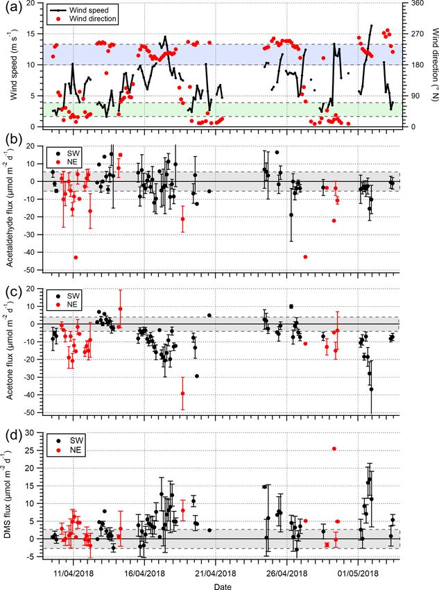
A time series of VOC fluxes (3 h average) is shown in al., 2011a).
Fig. 3. While acetone and DMS had clear unidirectional
fluxes (deposition and emission respectively), acetaldehyde 3.2 Seawater concentration and atmospheric mixing
showed bidirectional fluxes throughout the campaign. EC ratios of VOCs
fluxes of acetone, acetaldehyde, DMS and isoprene from the
two marine wind sectors averaged over the entire campaign The seawater concentrations of acetone, acetaldehyde and
are summarised in Table 1, with positive fluxes representing DMS measured around the campaign (Table A4) are broadly
net sea-to-air emission. similar (≤ 48 % difference) to previous measurements in the
For the open-water sector, acetone and DMS fluxes had western English Channel (Archer et al., 2009; Beale et al.,
relative standard errorsD. P. Phillips et al.: Air–sea exchange of acetone, acetaldehyde, DMS and isoprene 10117 Figure 3. Time series of 3 h averages of (a) wind speed (U10 ) and wind direction, (b) acetaldehyde flux, (c) acetone flux and (d) DMS fluxes for the open-water (180–240◦ N) and Plymouth Sound (30–70◦ N) wind sectors that met quality control criteria. Error bars are 1 standard error. The blue and green shaded zone in panel (a) represent the two wind sectors. The grey shaded zones in panels (b)–(d) represent limits of detection for 3 h averages, 5.8, 4.0 and 2.7 µmol m−2 d−1 for acetaldehyde, acetone and DMS respectively. mixing ratios of ∼ 0.16 and 0.44 ppbv, respectively. Finally, (Stein et al., 2015; Rolph et al., 2017) backward trajecto- rooftop measurements at PML (∼ 350 m north of the Ply- ries suggest that the air mass sampled on 1 May 2018 made mouth Sound, ∼ 6 km NE of the PPAO, and affected by lo- contact with land (mainland UK) ∼ 24–48 h prior to arriving cal ship/port activities) showed night-time atmospheric mix- at the PPAO (Fig. S4). Lewis et al. (2005) show that simi- ing ratios of ∼ 0.4 and ∼ 0.1 ppbv, respectively for acetone lar air-mass trajectories over the UK and continental Europe and acetaldehyde (Yang et al., 2013c). A summary of these contained high acetone levels (max of ∼ 1.67 ppbv). concentrations, in coordinate form, can be found in Fig. S3. Our mean DMS mixing ratio (0.20 ± 0.09, Table 2) is The atmospheric carbonyl measurements at the PPAO from in agreement with shipboard measurements in the east- this day might not represent purely oceanic conditions, even ern North Atlantic Ocean in June and July (0.16 ± 0.14 though wind was from the open-water sector. HYSPLIT and 0.12 ± 0.08 ppbv, with and without a phytoplankton https://doi.org/10.5194/acp-21-10111-2021 Atmos. Chem. Phys., 21, 10111–10132, 2021
10118                                    D. P. Phillips et al.: Air–sea exchange of acetone, acetaldehyde, DMS and isoprene

Figure 4. Histogram of (a) wind speed (U10 ) and (b) acetone and (c) DMS atmospheric gas-phase mixing ratio over the entire campaign.
Histograms are normalised for probability density separately and then to the same relative maximum occurrence. The gas mixing ratio
calculations here use extrapolated blanks here, which introduce some uncertainty; however the two wind sectors can still be compared.

bloom, respectively; Huebert et al., 2010) and the west-             3.3   Comparison between EC and bulk TL fluxes and
ern North Atlantic Ocean in March (0.13 ± 0.04; Quinn et                   derivation of the gas transfer velocities
al., 2019). Our mean isoprene mixing ratio (0.18 ± 0.05) is
higher than observations in autumn from the western North            Here we compare EC fluxes of acetone, acetaldehyde and
(0.035 ± 0.025 ppbv; Kim et al., 2017) and eastern North             DMS from the open-water sector with fluxes computed with
(0.0044 ± 0.0083 ppbv; Hackenberg et al., 2017) Atlantic             the TL model (using concurrent atmospheric mixing ratios
Ocean. The PPAO isoprene mixing ratio is more similar to             from the PPAO and linearly interpolated seawater concentra-
measurements at the Mace Head Observatory (Carslaw et al.,           tions from L4). This is to assess two assumptions in the TL
2000), which further implies some influence from terrestrial         flux calculation: (1) that gas transfer velocity parameterisa-
land sources at the PPAO site. We note that the TL air–sea           tions from deeper water (i.e. the open ocean or shelf seas) are
isoprene flux is almost purely governed by its seawater con-         applicable to this shallower coastal environment, and (2) sea-
centration where it is grossly supersaturated; the flux is in-       water VOC concentrations in the PPAO flux footprint and at
sensitive to the elevated atmospheric mixing ratio.                  the L4 station are similar.
                                                                        Acetone and acetaldehyde were both undersaturated in
                                                                     seawater in the open-water sector (Table 2), while DMS and
                                                                     isoprene were both supersaturated. The mean TL fluxes of

Atmos. Chem. Phys., 21, 10111–10132, 2021                                            https://doi.org/10.5194/acp-21-10111-2021
D. P. Phillips et al.: Air–sea exchange of acetone, acetaldehyde, DMS and isoprene 10119
DMS (16.7 ± 2.7 cm h−1 ) is in good agreement when com-
pared to published measurements (∼ 17 cm h−1 ; Blomquist
et al., 2006; Yang et al., 2011a; Bell et al., 2013) at sim-
ilar wind speeds in the North Atlantic Ocean. Data from
this short campaign suggest that the mean wind speed de-
pendence in DMS transfer velocity at the PPAO (open-water
sector, depth of ∼ 20 m) is largely comparable to deeper wa-
ter, in agreement with previous CO2 gas exchange measure-
ments at this site (Yang et al., 2019a). Our measured acetone
and acetaldehyde Ka are also of the expected magnitudes.
Processes important for shallow estuaries, such as bottom-
driven turbulence and tidal current, do not appear to be the
main controlling factors in gas exchange in this environment.
There is a large amount of scatter in Fig. 7, especially for
acetone and acetaldehyde. This is likely in part due to the
poor temporal resolution (weekly) in seawater concentration
Figure 5. A comparison between EC and bulk TL fluxes (hourly) measurements that do not capture any rapid changes in this
for the open-water sector during the dates 27 April–3 May 2018. dynamic region (e.g. changes in riverine outflow, biological
The error on EC measurements is 1 SE, whilst the error on TL is the bloom). Our DMS transfer velocity measurements imply that
propagated error of 1 SD in concentration and solubility. the outflow of the estuary Tamar does not substantially di-
lute the seawater DMS concentration within the open-water
flux footprint compared to L4, while spatial gradients in the
acetone, acetaldehyde, DMS and isoprene (n = 20) are pro- carbonyl concentrations could be more significant relative
vided in Table 2 with corresponding EC measurements from to their air–sea concentration differences. Higher resolution
the open-water wind sector for the last week of the campaign measurements within the flux footprints in the future are
(27 April–3 May 2018). For this short period with satisfac- needed to better constrain the influence of riverine outflow.
tory VOC blanking, the open-water EC fluxes were fairly As mentioned in Sect. 2.5, this paper uses a revised ace-
large in part because of a 17 % higher mean wind speed com- tone solubility from Wohl et al. (2020). Focusing on the last
pared to the rest of the campaign. week of the campaign (Table 2), we compute a mean TL
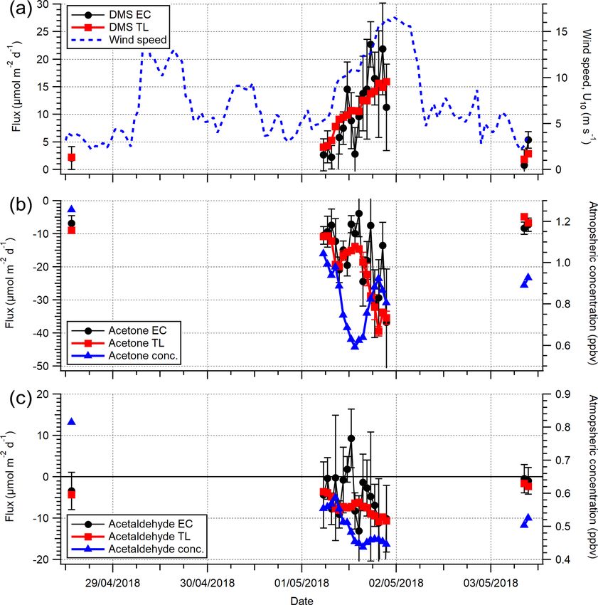
Figure 5 compares the VOC EC and TL fluxes for the acetone flux of −19.0 ± 2.2 and −21.5 ± 2.5 µmol m−2 d−1
open-water sector (not inc. isoprene), and Fig. 6 shows the (± SD, propagated error in concentration only) with and
same data as a time series. Acetone, acetaldehyde and DMS without the solubility revision. The flux with revised sol-
fluxes exhibit reasonable agreement between the EC and TL ubility is in better agreement with the EC measurement
methods, with both covarying with wind speed. The data (−14.9 ± 2.1 µmol m−2 d−1 ).
points furthest from the 1 : 1 line in Fig. 5 are hourly av-
erages with ≤ 2 10 min flux segments, suggesting that the 3.4 Comparison to other flux estimates
discrepancy is mainly due to random noise in the flux mea-
surement. We do not attempt to calculate TL fluxes for the The acetone fluxes presented here are in good agreement
Plymouth Sound sector because we do not have concurrent with previous EC measurements (−7.0 ± 2.2 µmol m−2 d−1 )
seawater measurements and have limited EC measurements from 50◦ N on an Atlantic Meridional Transect (AMT) re-
for comparison. search cruise in Autumn 2012 (Yang et al., 2014b). How-
To assess the wind speed dependence in gas transfer veloc- ever, the acetaldehyde flux here shows an opposite mean
ities at the PPAO, Ka is calculated by equating the EC flux direction to their 50◦ N average (1.8 ± 1.3 µmol m−2 d−1 ).
with TL flux; ρa w0 x 0 = −Ka (Ca − H Cw ). Figure 7 shows Acetone and acetaldehyde bulk fluxes from 50◦ N dur-
the calculated Ka and Kw (Kw = H Ka ) values for acetone, ing an AMT cruise in 2009, estimated using CAM-Chem
acetaldehyde and DMS using 1 h flux data, compared to cal- modelled atmospheric concentrations, were −5.7 ± 1.1 and
culated K from parameterisations of ka and kw . In the mean, −2.4 ± 0.7 µmol m−2 d−1 respectively (Beale et al., 2013).
the expected solubility dependence in these VOCs is ob- The PPAO fluxes are in reasonable agreement with these
served – the measurements show mean Ka of 2121, 1894 earlier indirect estimates. Further acetone and acetalde-
and 183 cm h−1 for acetone, acetaldehyde and DMS (in or- hyde bulk fluxes estimated from a time series of L4 wa-
der of decreasing solubility), respectively. These translate to ter measurements and static atmospheric mixing ratios
Kw values of 2.0, 2.6 and 9.9 cm h−1 . (0.66 and 0.40 ppbv respectively) were −7.4 ± 1.4 and
For DMS, to facilitate comparison with previous measure- 1.4 ± 1.0 µmol m−2 d−1 , respectively, for spring 2011 and
ments, the derived Kw is adjusted to a standard Schmidt num- −6.4 ± 0.1 and −1.5 ± 0.1 µmol m−2 d−1 , respectively, as
ber of 660 (K660 = Kw (660/SCw )−0.5 ). The mean K660 for annual averages. The spring acetone fluxes of Beale et
https://doi.org/10.5194/acp-21-10111-2021 Atmos. Chem. Phys., 21, 10111–10132, 202110120 D. P. Phillips et al.: Air–sea exchange of acetone, acetaldehyde, DMS and isoprene
Table 2. Saturations and two-layer bulk fluxes of VOCs in open-water (SW) and Plymouth Sound (NE) water (27 April–3 May 2018) along
with the eddy covariance measurements for this period. Errors for water concentration and air mixing ratio (measurement) and saturation
(propagation) indicate one standard deviation. Errors for flux indicate one standard error.
Compound Open water Plymouth Sound
Water Air mixing Saturation TL flux EC flux Air mixing EC flux
conc. (nM) ratio (ppbv) (%) (µmol m−2 d−1 ) (µmol m−2 d−1 ) ratio (ppbv) (µmol m−2 d−1 )
Acetaldehyde 7.1 ± 1.4 0.51 ± 0.07 44 ± 6 −6.76 ± 0.59 −3.94 ± 1.23 0.75 ± 0.04 −7.32 ± 2.86
Acetone 5.3 ± 2.0 0.82 ± 0.16 15 ± 3 −18.98 ± 2.24 −14.93 ± 2.09 1.09 ± 0.09 −8.21 ± 4.00
DMS 3.6 ± 0.8 0.20 ± 0.09 1434 ± 569 9.41 ± 1.03 9.61 ± 1.55 0.015 ± 0.006 2.55 ± 2.36
Isoprene 0.09 ± 0.01 0.18 ± 0.05 971 ± 221 0.30 ± 0.05 1.65 ± 1.89 0.28 ± 0.03 9.27 ± 3.01
Figure 6. A comparison between (a) DMS, (b) acetone and (c) acetaldehyde EC and TL fluxes (hourly) for the open-water sector during
the dates 27 April–3 May 2018. Wind speed (U10 ) is provided in (a). The error on EC measurements is 1 SE, whilst the error on TL is the
propagated error of 1 SD in concentration and solubility.
al. (2015) are in good agreement with the PPAO direct mea- mixing ratio are probably among the main causes for the dis-
surements; however their acetaldehyde flux was in the oppo- crepancies in these air–sea flux estimates (Yang et al., 2014b,
site direction. Importantly, Beale et al. (2015) identified that Beale et al., 2013, 2015, and PPAO measurements presented
the L4 water saturation of acetaldehyde was highly sensitive here).
to the atmospheric mixing ratio (changing it between 0.1– The PPAO DMS flux is in agreement with previ-
0.4 ppbv was enough to switch the direction of flux). Thus ous EC DMS flux observations from the eastern North
variability and uncertainty in the atmospheric acetaldehyde Atlantic Ocean during summer 2007 (4.4 ± 0.4 and
Atmos. Chem. Phys., 21, 10111–10132, 2021 https://doi.org/10.5194/acp-21-10111-2021D. P. Phillips et al.: Air–sea exchange of acetone, acetaldehyde, DMS and isoprene 10121
Figure 7. Calculated transfer velocities (hourly) for (a) DMS (Kw,600 ), (b) acetone (Ka ) and (c) acetaldehyde (Ka ) in the open-water foot-
print of the Penlee Point Atmospheric Observatory during the dates 27 April–3 May 2018. Error bars on the experimental data (black circles)
are propagated uncertainty from the eddy covariance measurement. The black poly fit lines are fit to the experimental data, with the dashed
black lines representing 95 % confidence in the poly fit. The red circle and blue triangle lines in panel (a) are theoretical transfer velocities
using the kw parameterisations of Yang et al. (2011a) and Nightingale et al. (2000) respectively. The red circle lines in panels (b) and (c) are
theoretical transfer velocities calculated from the kw parameterisation of Yang et al. (2011a) and ka from the COAREG 3.5 model (shown as
blue triangles).
2.6 ± 0.2 µmol m−2 d−1 with and without a short, intense tions in the North Atlantic Ocean without the phytoplankton
phytoplankton bloom; Huebert et al., 2010). Our campaign bloom (5.58 ± 0.15 µmol m−2 d−1 ; Bell et al., 2013).
ended before the spring phytoplankton bloom started at L4 Although isoprene EC fluxes were unresolvable, the esti-
(Archer et al., 2009), which typically starts in May or June. mated open-water TL flux was similar to NECS April esti-
Yang et al. (2016c) estimated bulk DMS fluxes of 3 and mates of ∼ 0.8 µmol m−2 d−1 (Palmer and Shaw, 2005) and
10 µmol m−2 d−1 in the winter and summer, respectively, us- ∼ 1.0 µmol m−2 d−1 (Booge et al., 2016, supplement) using
ing the L4 annual seawater DMS concentration time series MODIS satellite observations of chlorophyll a for production
(Archer et al., 2009). The DMS flux measurement at the models. A mean direct flux (0.7 µmol m−2 d−1 ) was observed
PPAO is also in reasonable agreement with previous observa- in the northern North Atlantic Ocean (Kim et al., 2017); Kim
et al. (2017) estimated seawater concentrations (∼ 0.02 nM)
https://doi.org/10.5194/acp-21-10111-2021 Atmos. Chem. Phys., 21, 10111–10132, 202110122 D. P. Phillips et al.: Air–sea exchange of acetone, acetaldehyde, DMS and isoprene that were ∼ 78 % lower than measured here but also expe- use of a constant lifetime of 0.3 d for the global ocean, rienced much higher wind speed. Importantly, discrepancies whereas previous measurements at L4 suggest a much between top-down and bottom-up isoprene budget analyses shorter acetaldehyde lifetime (0.01–0.13 d; Beale et al., show the ocean fluxes necessary to explain remote marine 2015). de Bruyn et al. (2017) showed shorter seawater boundary layer (MBL) concentrations of isoprene are an or- acetaldehyde lifetimes at another coastal location directly der of magnitude higher than predicted from seawater con- after rainfall or during the wet season. It is possible that centrations alone (Arnold et al., 2009; Booge et al., 2016). the shorter lifetime at L4/PPAO, and hence lower seawater Future simultaneous comparisons between EC and TL iso- acetaldehyde concentration, may be related to riverine prene fluxes might observe this difference. input. The atmospheric acetaldehyde mixing ratios from We also compare our direct VOC fluxes to global model the models are also lower than the coastal observations predictions at this location. Typical global models and cli- presented here, similar to acetone as discussed above. matologies operate with a 1◦ latitudinal and longitudinal res- From the perspective of climatology and global mod- olution (e.g. Wang et al., 2019, 2020a, b). At the PPAO, this elling, the NECS was predicted to have an April DMS equates to a grid size of ∼ 110 km N–S and ∼ 85 km E–W, flux of ∼ 14 µmol m−2 d−1 (Lana et al., 2011) and which is much coarser compared to the flux footprint areas ∼ 6 µmol m−2 d−1 (Wang et al., 2020b). The estimate of (on the order of a few square kilometres). Nevertheless, this Lana et al. (2011) is 3 times higher than the PPAO measure- comparison allows us to qualitatively assess the spatial repre- ments; however that of Wang et al. (2020b) is in good agree- sentativeness of the PPAO fluxes and identify potential short- ment. Waterside concentrations of ∼ 7 and ∼ 3 nM were pre- comings in the models. dicted (52 % higher and 43 % lower than the L4 concentra- The GEOS-Chem and CAM-Chem models predict tion) by Lana et al. (2011) and Wang et al. (2020b) respec- a mean annual acetone flux in the eastern North tively. The high concentrations in the Lana et al. (2011) cli- Atlantic Ocean coastal shelves (NECS; biogeochemi- matology likely correspond to phytoplankton blooms in the cal province that includes the PPAO coastal site) of April–May period, which did not occur at the time of our ∼ −2.5 µmol m−2 d−1 (Fischer et al., 2012) and March–May measurements or appear as intensely in the estimations of flux of ∼ −2.9 µmol m−2 d−1 (Wang et al., 2020a), respec- Wang et al. (2020b). This could be partly related to the inter- tively. These two predictions are much lower than measured annual variability in plankton dynamics and hence seawater in the PPAO open-water sector (−8.01 ± 0.77 µmol m−2 d−1 , DMS cycling. Table 1) because the models predict a smaller air–sea con- All the models and climatologies discussed here (except centration difference. Fisher et al. (2012) and Wang et for Wang et al., 2020b) used the Nightingale et al. (2000) kw al. (2020a) used water concentrations of 15 (static) and parameterisation, which leads to ∼ 26 %, ∼ 14 % and ∼ 26 % ∼ 8 nM respectively (182 % and ∼ 50 % higher than L4 con- higher kw values for acetone, acetaldehyde and DMS, respec- centrations) and a modelled atmospheric mixing ratio of tively, than those of Yang et al. (2011a) over this campaign ∼ 0.45 ppbv (∼ 45 % lower than the PPAO concentration). because of the solubility dependence in bubble-mediated gas Seawater acetone has a highly variable lifetime (Beale et al., exchange (Yang et al., 2011a; Bell et al., 2017). Substitut- 2013; de Bruyn et al., 2013; Dixon et al., 2013), so the higher ing the Nightingale et al. (2000) kw parameterisation with estimated seawater concentration in the Wang et al. (2020a) the Yang et al. (2011a) kw would generally reduce the flux model may be because of a slower removal rate. We mea- magnitude in these models, estimated as ∼ 5 %, ∼ 6 % and sured an atmospheric acetone mixing ratio that is higher than ∼ 19 % for acetone, acetaldehyde and DMS, respectively (ka in the model likely because our measurement, even from the unchanged and from COAREG 3.5). open-water sector, has some terrestrial influence (e.g. via the diurnal sea-breeze effect or advection of air masses previ- 3.5 Significance of fluxes ously in contact with land). The small negative acetaldehyde fluxes measured Our measured open-water acetone and acetaldehyde air– at the PPAO imply a weak ocean sink (mean of sea fluxes exhibit stronger deposition flux than estimated −1.55 ± 1.14 µmol m−2 d−1 , Table 1), which does not by global modelling. Here we evaluate the lifetimes of agree with global model results. The NECS acetaldehyde these gases within the atmospheric MBL. The MBL life- flux is ∼ 0.22 µmol m−2 d−1 in GEOS-Chem (Millet et al., times (τx ) are calculated similarly to a 0D model; τx = 2010) and ∼ 1.4 µmol m−2 d−1 in CAM-Chem (Wang et Cx /(Cx Lx + Dx / h), where Cx represents concentration al., 2019) in the March–May period. The seawater concen- (here, the mean of the PPAO observations; Table 2), Lx trations used by Wang et al. (2019) (∼ 11 nM) are higher represents chemical loss, Dx represents the net deposition than L4 measurements for the same period (54 % higher flux (here, the mean of the PPAO EC observations; Ta- than L4 conc.). In the model, the short marine lifetime of ble 1) and h represents MBL height. We assume h to be acetaldehyde (de Bruyn et al., 2013, 2017; Dixon et al., 500 m and VOCs to be homogeneously mixed within the 2013) is coupled with an estimate of its production rate MBL upwind of the PPAO, and Lx is 2.7 × 10⁻⁷ s−1 for to predict the seawater concentration. Wang et al. (2019) acetone and 2.1 × 10⁻⁵ s−1 for acetaldehyde. Lx is calcu- Atmos. Chem. Phys., 21, 10111–10132, 2021 https://doi.org/10.5194/acp-21-10111-2021
D. P. Phillips et al.: Air–sea exchange of acetone, acetaldehyde, DMS and isoprene                                          10123

lated from literature OH reaction rates (1.7 × 10⁻¹³ and           fluxes of acetone and acetaldehyde from the latter because of
1.5 × 10⁻¹¹ cm3 molec.−1 s−1 , respectively; Atkinson and          higher atmospheric carbonyl concentrations from that wind
Arey, 2003), April surface 50◦ N zonal average OH concen-          direction. Emission fluxes of DMS from the terrestrially in-
tration (∼ 106 molec. cm−3 ; Horowitz et al., 2003) and sum-       fluenced sector are weaker than from the open-water sector,
mer surface photolysis rates for acetone (∼ 10−7 s−1 ; Blitz et    likely because of lower wind speeds and lower seawater con-
al., 2004) and acetaldehyde (∼ 5.5 × 10⁻⁶ s−1 ; Warneck and        centrations due to estuarine influence/dilution.
Moortgat, 2012).                                                      Bulk fluxes computed from seawater and atmospheric con-
   From this simple model and the values described above,          centrations using the TL approach agree reasonably well with
the MBL lifetimes of acetone and acetaldehyde are calcu-           our EC measurements of open-water acetone, acetaldehyde
lated to be 2.0 and 0.5 d respectively. The deposition to the      and DMS fluxes. The derived air–sea transfer velocities of
ocean above accounts for 95 % and 8 % of all losses for            acetone, acetaldehyde and DMS are largely consistent with
MBL acetone and acetaldehyde respectively, which high-             previous estimates over the open ocean in the mean. Along
lights the importance of acetone air–sea exchange. The calcu-      with previous measurements of air–sea CO2 exchange, these
lated PPAO open-water acetone lifetime is much shorter than        data suggest that wind, rather than processes such as bottom
the 11–18 d estimates for the mean troposphere (Marandino          driven turbulence, is the dominant control for gas exchange
et al., 2005; Fischer et al., 2012; Khan et al., 2015; Wang        at this site for the open-water sector (depth of ∼ 20 m).
et al., 2020a), where surface deposition is less substantial          While the DMS flux at PPAO was in reasonable agree-
(16 %–56 %; Jacob et al., 2002; Fischer et al., 2012). The         ment with recent climatological estimates, our measured
acetaldehyde lifetime is in good agreement with literature         open-water acetone fluxes show stronger deposition com-
values (0.1–0.8 d; Millet et al., 2010; Wang et al., 2019) be-     pared to climatological and model estimates for the NE At-
cause photochemistry is the main loss mechanism for MBL            lantic Ocean coastal shelf. This is likely because the mod-
acetaldehyde rather than deposition, and the April surface         els/climatologies do not fully capture the spatial and tem-
50◦ N zonal average OH concentration is similar to the tro-        poral variability in the distribution of atmospheric and sea-
pospheric mean (1.1 × 10⁶ molec. cm−3 ; Li et al., 2018).          water acetone concentrations. The PPAO acetaldehyde flux
   The noticeable increase in acetone and acetaldehyde de-         (net sink in the mean) is in the opposite direction to global
position fluxes within the Plymouth Sound compared to the          models that suggest the Northern Hemisphere oceans to be a
open-water sector suggests that deposition can represent a         net acetaldehyde source. This is mostly because models pre-
large loss term for atmospheric VOCs in the coastal atmo-          dict higher seawater acetaldehyde concentrations and lower
sphere. Importantly, enhanced coastal deposition fluxes of         atmospheric acetaldehyde mixing ratios at this coastal loca-
acetone and acetaldehyde are not well captured in global           tion.
models. The boundary layer lifetimes during periods of off-           Future experiments at PPAO should strive to increase the
shore winds are calculated using the same approach as be-          temporal and spatial resolutions of the Cw observations in or-
fore, resulting in 1.7 d for acetone and 0.5 d for acetaldehyde.   der to better match up with the EC fluxes. The accuracies in
Here deposition to the ocean accounts for 96 % and 17 % of         the air and water concentration measurements can be further
losses, respectively. The estimated lifetimes in the Plymouth      improved by using blanks that have the same CO2 and hu-
Sound sector are similar to the open ocean even though the         midity levels as the samples, especially for acetaldehyde. The
deposition fluxes were stronger because the increased depo-        use of a higher resolution PTR-time-of-flight-MS at ≥ 10 Hz
sition fluxes correspond to a greater atmospheric burden. As       would improve the precision of the flux measurement and re-
air masses from the Plymouth Sound (or further inland to the       duce the magnitude of the high-frequency flux loss. Simulta-
NE) are advected offshore over the coastal seas, the mixing        neous methanol fluxes would enable the derivation of the air-
ratios of carbonyls tend to decrease due to combination of         side gas transfer velocity (ka ) and benefit the lag correlation
deposition to the sea, chemical losses and mixing with ma-         calculation (methanol flux is typically large; see Yang et al.,
rine air. If additional x–y dimensional constraints are added      2014a). Important future work would involve measuring EC
to the Plymouth Sound 0D box (e.g. 4 km N–S, 1 km E–W),            fluxes, Cw and Ca at high resolution from the anthropogeni-
dilution becomes an important loss term.                           cally/terrestrially dominated coast through to the continental
                                                                   shelf edge and open ocean on a ship in order to develop our
                                                                   understanding of the impact of coastal seas on local atmo-
4   Conclusions                                                    spheric chemistry and quality. Such transect measurements
                                                                   would help to further constrain global models for improved
This paper presents measurements of air–sea fluxes of ace-         estimations at the coast.
tone, acetaldehyde and DMS at the coastal PPAO in the SW
UK. A PTR-quadrupole-MS (2.2 Hz) was used to simultane-
ously resolve the fluxes of these gases with the eddy covari-
ance method. Comparisons between the open-water sector
and a terrestrially influenced sector show stronger deposition

https://doi.org/10.5194/acp-21-10111-2021                                        Atmos. Chem. Phys., 21, 10111–10132, 2021
10124 D. P. Phillips et al.: Air–sea exchange of acetone, acetaldehyde, DMS and isoprene
Appendix A: Additional eddy covariance method details Random uncertainty in the EC flux depends on variabil-
ity (instrument noise + ambient variability) in the VOC mea-
Table A1 shows the PTR–MS measurement parameters used, surement and the wind measurement. Precision (or random
which largely follows from Yang et al. (2013c). Importantly, error) in the EC technique can be approximated as the stan-
a high drift voltage was used to limit the formation of hy- dard deviation of “null” fluxes (i.e. covariance data with a
drated clusters (H3 O+ +nH2 O −→ H3 O+ (H2 O)n ) caused by lag time between vertical wind and concentration measure-
the high humidity of marine air. These hydrated clusters have ments that is much greater than the integral timescale; Spirig
different reaction kinetics with VOCs and can affect the in- et al., 2005). Fluxes are resolvable when they are higher than
strumental sensitivity. Increasing the drift voltage leads to a 3 times the measurement noise. An artificial lag time of 300 s
lower cluster formation but also causes a greater degree of was chosen for this calculation here. The 3 times standard
isoprene fragmentation (Schwarz et al., 2009; Wohl et al., deviation was calculated from hourly averages over a 5 h
2019). Isoprene fragmentation was corrected using gas-phase window of stable open-water wind speed and direction as
calibration. 10.1, 6.8, 4.7 and 4.7 µmol m−2 d−1 , for acetaldehyde, ace-
Table A2 shows the quality control criteria used to fil- tone, DMS and isoprene respectively. Our LOD estimates are
ter 10 min flux data segments, developed from EC measure- 140 %–250 % of the LOD from a previous deployment of this
ments of CO2 and CH4 fluxes at the PPAO (Yang et al., PTR-MS at sea (Yang et al., 2014b), mainly due to the greater
2016a). Standard deviation in wind direction was used to en- ambient variability in VOC mixing ratio at this coastal envi-
sure fairly constant wind direction and minimise influence ronment. Hourly data√were averaged to 3 h to reduce random
from areas outside the specified NE and SW wind sectors. error by a factor of 3; thus the 3 h LOD are 5.8, 4.0, 2.7
The remaining controls check for the stationary criteria re- and 2.7 µmol m−2 d−1 , for acetaldehyde, acetone, DMS and
quired for EC measurements, remove periods with obvious isoprene respectively.
flow distortion or remove periods with substantial rain influ-
ence on the sonic anemometer. Table A2. Flux segment quality control criteria.
Table A1. PTR–MS method used for measurements. Parameter Value
Parameter Value Wind direction [σ ] (◦ )You can also read