Conditioning ensemble streamflow prediction with the North Atlantic Oscillation improves skill at longer lead times - HESS
←
→
Page content transcription
If your browser does not render page correctly, please read the page content below
Hydrol. Earth Syst. Sci., 25, 4159–4183, 2021
https://doi.org/10.5194/hess-25-4159-2021
© Author(s) 2021. This work is distributed under
the Creative Commons Attribution 4.0 License.

Conditioning ensemble streamflow prediction with the North
Atlantic Oscillation improves skill at longer lead times
Seán Donegan1 , Conor Murphy1 , Shaun Harrigan2 , Ciaran Broderick3 , Dáire Foran Quinn1 , Saeed Golian1 ,
Jeff Knight4 , Tom Matthews5 , Christel Prudhomme2,5,6 , Adam A. Scaife4,7 , Nicky Stringer4 , and Robert L. Wilby5
1 IrishClimate Analysis and Research UnitS (ICARUS), Department of Geography,
Maynooth University, Maynooth, Co. Kildare, Ireland
2 Forecast Department, European Centre for Medium-Range Weather Forecasts (ECMWF), Reading, UK
3 Flood Forecasting Division, Met Éireann, Dublin 9, Ireland
4 Met Office Hadley Centre, Exeter, UK
5 Department of Geography and Environment, Loughborough University, Loughborough, UK
6 UK Centre for Ecology & Hydrology (UKCEH), Wallingford, UK
7 College of Engineering, Mathematics, and Physical Sciences, University of Exeter, Exeter, UK

Correspondence: Seán Donegan (sean.donegan@mu.ie)

Received: 19 November 2020 – Discussion started: 14 December 2020
Revised: 13 May 2021 – Accepted: 5 June 2021 – Published: 22 July 2021

Abstract. Skilful hydrological forecasts can benefit            responding, high-storage catchments are located. Forecast
decision-making in water resources management and other         reliability and discrimination were also assessed with
water-related sectors that require long-term planning. In       respect to low- and high-flow events. In addition to our
Ireland, no such service exists to deliver forecasts at the     benchmarking experiment, we conditioned ESP with the
catchment scale. In order to understand the potential for       winter North Atlantic Oscillation (NAO) using adjusted
hydrological forecasting in Ireland, we benchmark the skill     hindcasts from the Met Office’s Global Seasonal Forecasting
of ensemble streamflow prediction (ESP) for a diverse           System version 5. We found gains in winter forecast skill
sample of 46 catchments using the GR4J (Génie Rural             (CRPSS) of 7 %–18 % were possible over lead times of 1
à 4 paramètres Journalier) hydrological model. Skill is         to 3 months and that improved reliability and discrimina-
evaluated within a 52-year hindcast study design over lead      tion make NAO-conditioned ESP particularly effective at
times of 1 d to 12 months for each of the 12 initialisation     forecasting dry winters, a critical season for water resources
months, January to December. Our results show that ESP          management. We conclude that ESP is skilful in a number
is skilful against a probabilistic climatology benchmark in     of different contexts and thus should be operationalised in
the majority of catchments up to several months ahead.          Ireland given its potential benefits for water managers and
However, the level of skill was strongly dependent on lead      other stakeholders.
time, initialisation month, and individual catchment location
and storage properties. Mean ESP skill was found to decay
rapidly as a function of lead time, with a continuous ranked
probability skill score (CRPSS) of 0.8 (1 d), 0.32 (2-week),    1   Introduction
0.18 (1-month), 0.05 (3-month), and 0.01 (12-month).
Forecasts were generally more skilful when initialised in       Skilful hydrological forecasts at lead times of weeks to
summer than other seasons. A strong correlation (ρ = 0.94)      months can benefit water resources management (Anghileri
was observed between forecast skill and catchment storage       et al., 2016; Dixon and Wilby, 2019; Viel et al., 2016; Wet-
capacity (baseflow index), with the most skilful regions,       terhall and Di Giuseppe, 2018) and help mitigate extreme
the Midlands and the East, being those where slowly             events by enhancing preparedness and improving operational
                                                                decisions (Luo and Wood, 2007; Neumann et al., 2018; Pap-

Published by Copernicus Publications on behalf of the European Geosciences Union.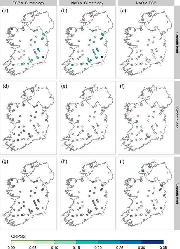
4160                 S. Donegan et al.: Conditioning ensemble streamflow prediction with the North Atlantic Oscillation

penberger et al., 2015a; Zhao and Zhao, 2014). For example,           ESP is a well-established forecasting technique in which
hydrological forecasts have been used to modify reservoir          historical sequences of climate data at the time of forecast are
operations for hydropower production (Fan et al., 2016), stor-     used to drive a hydrological model, producing an ensemble
age and supply (Turner et al., 2017), and the management of        of equiprobable future streamflow traces (Day, 1985; Twedt
flood and drought conditions (Amnatsan et al., 2018; Ficchì        et al., 1977). It is comparable to persistence in that it requires
et al., 2016; Watts et al., 2012). They have also been shown       no information about future meteorological conditions; out-
to benefit sectors such as agriculture (Mushtaq et al., 2012),     looks are instead based on knowledge of hydrological state
tourism (Fundel et al., 2013), and navigation (Meißner et al.,     variables (i.e. antecedent soil moisture, groundwater, snow-
2017). Such applications can yield significant economic re-        pack, and streamflow itself) which can provide predictabil-
turns. For instance, Hamlet et al. (2002) reported a poten-        ity up to 5 months ahead (Wood and Lettenmaier, 2008). In
tial rise in annual revenue of USD 153 million when fore-          this regard, ESP can be used to efficiently specify not only
cast information was incorporated into the operation of ma-        the catchments where knowledge of initial conditions or me-
jor hydropower dams in the Columbia River basin. Similarly,        teorological forcing may be the greatest source of skill, but
Pappenberger et al. (2015a) claim that the European Flood          also the time of year and lead times over which different skill
Awareness System (EFAS; Thielen et al., 2009) saves around         sources may be dominant (Wood and Lettenmaier, 2006).
EUR 400 for every EUR 1 invested.                                     The ESP method was originally developed in the snow-
   The value of hydrological forecasting has led several coun-     dominated catchments of the western United States (e.g.
tries to establish operational seasonal hydrological forecast-     Franz et al., 2003) but has shown skill in other regions,
ing (SHF) systems. These include the U.S. National Weather         including the UK (Harrigan et al., 2018), European Alps
Service’s (NWS) Hydrologic Ensemble Forecast Service               (Förster et al., 2018), Sweden (Girons Lopez et al., 2021),
(HEFS; Demargne et al., 2014), the Hydrological Outlook            New Zealand (Singh, 2016), Australia (Pagano et al., 2010;
UK (HOUK; Prudhomme et al., 2017), and the Australian              Wang et al., 2011), and China (Yuan et al., 2016). Simplic-
Bureau of Meteorology’s statistical and dynamical forecasts        ity and efficiency make ESP a popular choice for operational
(Schepen and Wang, 2015). Although Ireland benefits from           forecasting. It is one of three methods used in the HOUK
regional hydrological outlooks provided by EFAS, no ser-           (Prudhomme et al., 2017) and forms the basis of the NWS
vice currently exists for delivering forecasts at the catchment    HEFS (Demargne et al., 2014). Moreover, ESP is recognised
scale; yet water managers and other stakeholders require con-      as a low-cost, “tough-to-beat” forecast (Pappenberger et al.,
fident, locally tailored forecast information. A national oper-    2015b) against which value added by more sophisticated hy-
ational SHF system could bridge this gap. However, despite         drometeorological ensemble systems can be assessed (e.g.
interest from water managers, it is difficult to justify the im-   Arnal et al., 2018; Bazile et al., 2017; Wanders et al., 2019).
plementation of such a system as little preparatory work has       Hence, the potential application of ESP in Ireland merits ex-
been done to evaluate the potential for hydrological forecast-     ploration.
ing in an Irish context.                                              However, lack of sensitivity to concurrent meteorological
   Recent international assessments of progress in SHF (Tang       conditions limits the application of ESP in areas that are less
et al., 2016; Yuan et al., 2015) indicate that (i) advances in     dependent on the initial hydrological state. Given that lo-
empirical and dynamical SHF are feasible in climate contexts       cal meteorological conditions are known to be teleconnected
that resemble Ireland; and (ii) SHF spans a wide range of          to regional variations in atmospheric–oceanic modes, ESP
methods with varying complexity and data requirements, but         techniques may be improved by conditioning on these cir-
no universally accepted “best” approach has emerged. As the        culation patterns. Several studies have already demonstrated
performance of different methods will likely depend on time        the added value of incorporating climate information into
of year, lead time, and, critically, local hydrological context    ESP forecasts in this way. For example, Hamlet and Letten-
(Girons Lopez et al., 2021; Harrigan et al., 2018; Meißner         maier (1999) found that conditioning ESP traces according to
et al., 2017; Pechlivanidis et al., 2020), understanding how       El Niño–Southern Oscillation (ENSO) and Pacific Decadal
best to apply the range of available tools to develop skilful      Oscillation (PDO) indicators significantly improved forecast
forecasts for Ireland requires rigorous testing at the catch-      specificity and extended lead time by about 6 months in the
ment scale. To the authors’ knowledge, only Foran Quinn            Columbia River basin. Similarly, both Werner et al. (2004)
et al. (2021) have previously evaluated seasonal streamflow        and Bradley et al. (2015) reported improvements of 28 %
forecasts for Ireland. They found that whilst skill was mainly     and 27 % in forecast skill, respectively, when conditioning
restricted to summer months, statistical persistence forecasts     ESP with ENSO. More modest improvements of 5 %–10 %
could have practical value in the management of water re-          were observed by Beckers et al. (2016) for two test stations
sources and hydrological extremes. We build on this work           when applying an ENSO-conditioned ESP. More recently,
and further assess the scientific basis for SHF in Ireland by      Yuan and Zhu (2018) showed that decadal predictions of ter-
evaluating and benchmarking the skill of ensemble stream-          restrial water storage made using ESP could be improved by
flow prediction (ESP).                                             conditioning with PDO and Atlantic Multidecadal Oscilla-
                                                                   tion indices.

Hydrol. Earth Syst. Sci., 25, 4159–4183, 2021                                       https://doi.org/10.5194/hess-25-4159-2021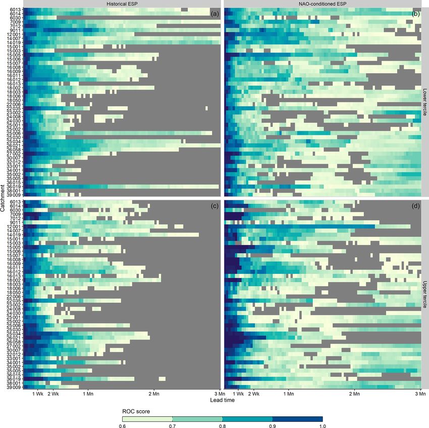
S. Donegan et al.: Conditioning ensemble streamflow prediction with the North Atlantic Oscillation                             4161

   In Europe, the dominant mode of climate variability is the
North Atlantic Oscillation (NAO). The NAO affects stream-
flow predictability, particularly during winter (Bierkens and
van Beek, 2009; Steirou et al., 2017; Wedgbrow et al., 2002;
Wilby, 2001), and it is highly correlated with winter stream-
flow over Ireland (Murphy et al., 2013). As winter is the
most important season for groundwater recharge in Europe,
the ability to accurately forecast winter streamflow would be
extremely beneficial for water managers. Advances in pre-
dicting the NAO (Scaife et al., 2014; Smith et al., 2020) en-
able long-range forecasts of UK winter hydrology (Svens-
son et al., 2015) as well as improved seasonal meteorologi-
cal forecasts for driving hydrological models (Stringer et al.,
2020). Hence, it may be possible to leverage this predictabil-
ity to improve ESP performance by sub-sampling ensemble
members for Ireland using the winter NAO.
   In this paper, we benchmark ESP skill against streamflow
climatology within a 52-year hindcast study design. Skill is
evaluated for a combination of different lead times and ini-       Figure 1. Location of the 46 study catchments, shaded by region,
tialisation months and for diverse hydroclimate regions and        and associated gauging stations (white dots).
catchment types. The relationship between catchment char-
acteristics and ESP skill is explored. Reliability and discrimi-
nation are assessed with respect to low- and high-flow events.     (iii) they had little evidence of land-use change; and (iv) to-
We also examine the effect of conditionally sampling ensem-        gether they build a representative sample of Ireland’s diverse
ble members on ESP skill during winter. The following re-          hydrological and climatological conditions, with good spatial
search questions are addressed:                                    coverage. This selection process ensured sufficient data for
                                                                   hydrological model calibration whilst limiting the potential
    1. When is ESP skilful, given a wide range of lead times
                                                                   for confounding factors that could adversely affect the in-
       and initialisation months?
                                                                   terpretation of results. Catchments were grouped according
    2. Where is ESP most skilful, at regional and catchment        to the European Union’s NUTS (Nomenclature of Territo-
       scales?                                                     rial Units for Statistics) III regions (Fig. 1) to explore spatial
                                                                   variations in skill. As the Dublin region contained only one
    3. How does ESP skill relate to catchment characteristics?     catchment in our sample, this was merged with the Mid-East
                                                                   into a single region: the East. The distribution of catchments
    4. To what extent can winter ESP skill be improved by
                                                                   within the seven regions ranges from four in the West to 10
       conditioning on the NAO?
                                                                   in the Mid-West. Although the NUTS III regions do not in-
    5. What is the potential for operationalising the ESP          herently lend themselves to hydrological analysis, grouping
       method for hydrological forecasting in Ireland?             the catchments in this way did yield regions that were diverse
                                                                   in terms of their hydrology and climate. They are therefore
   Section 2 describes our data and methods. Our results are       suitable to examine how skill may differ between areas with
presented in Sect. 3. We offer discussion and suggestions          contrasting hydroclimate properties.
for future research in Sect. 4. Conclusions are presented in          Observed daily mean streamflow data (m3 s−1 ) were ob-
Sect. 5.                                                           tained from gauging stations administered by the Office
                                                                   of Public Works (OPW) and the Environmental Protection
2     Data and methods                                             Agency. Despite the strict selection criteria, some catchments
                                                                   still contain multiple or extended periods of missing data.
2.1    Catchment selection and observed data                       Hence, streamflow records were retrieved only for calen-
                                                                   dar years 1992–2017 – the longest usable period common
A total of 46 catchments were selected for our analysis fol-       to all 46 catchments. Catchment average daily precipitation
lowing the same criteria used to establish the Irish Reference     (mm d−1 ) and temperature (◦ C) spanning 1961–2017 were
Network (Murphy et al., 2013). Catchments were selected            derived from gridded (1 km × 1 km) datasets developed by
provided they met the following conditions: (i) they had           Met Éireann (Walsh, 2012). Potential evaporation (mm d−1 )
quality-assured, long-term observational data, with a mini-        was calculated from temperature and radiation according to
mum record length of 25 years; (ii) they had a flow regime         Oudin et al. (2005).
which had not been significantly altered by human activity;

https://doi.org/10.5194/hess-25-4159-2021                                       Hydrol. Earth Syst. Sci., 25, 4159–4183, 2021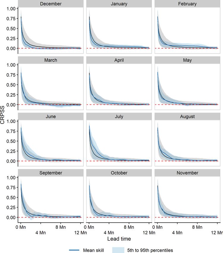
4162                   S. Donegan et al.: Conditioning ensemble streamflow prediction with the North Atlantic Oscillation

Table 1. Physical catchment descriptors referred to in this study.

              Descriptor     Explanation                                                                    Units    Range
              BFI            Baseflow index; proportion of runoff derived from stored sources               –          0–1
              RBI            Richards–Baker flashiness index; oscillations in flow relative to total flow   –          0–1
              RR             Runoff ratio; ratio of runoff to received precipitation                        –          0–1
              AREA           Catchment area                                                                 km2          –
              SAAR           Standard-period (1961–1990) average annual rainfall                            mm           –
              FLATWET        Proportion of time soils expected to be typically quite wet                    –          0–1
              PEAT           Proportional extent of catchment area classified as peat bog                   –          0–1
              FOREST         Proportional extent of forest cover                                            –          0–1
              MSL            Main-stream length                                                             km           –
              S1085          Slope of main stream excluding the bottom 10 % and top 15 % of its length      m km−1       –
              TAYSLO         Taylor–Schwartz measure of main-stream slope                                   m km−1       –

   Data on catchment physical attributes were based on a se-             for Ireland and each of the NUTS III regions in Table 2 and
lection of physical catchment descriptors (PCDs) from the                for individual catchments in Table S1 in the Supplement.
OPW’s Flood Studies Update (Mills et al., 2014). These
PCDs describe facets of catchment hydrology, morphology,                 2.2   Hydrological modelling
soil, and climate and are used here to examine relationships
between catchment characteristics and ESP skill. The pri-                The GR4J (Génie Rural à 4 paramètres Journalier; Perrin
mary PCDs of interest are the baseflow index (BFI), the                  et al., 2003) daily lumped conceptual rainfall-runoff model
Richards–Baker flashiness index (RBI; Baker et al., 2004),               was applied. This model has a parsimonious structure con-
and the runoff ratio (RR), as these describe aspects of catch-           sisting of four free parameters (x1 –x4 ) that require calibra-
ment storage and response and have been linked to ESP                    tion of observed streamflow data against precipitation and
skill (e.g. Girons Lopez et al., 2021; Harrigan et al., 2018;            potential evaporation. The model structure can be described
Pechlivanidis et al., 2020). The BFI is calculated according             in terms of its water balance and routing operators (Santos
to the Institute of Hydrology method (Gustard et al., 1992)              et al., 2018). Water is partitioned between a production (soil
and quantifies the contribution of stored sources to runoff.             moisture accounting) store and a routing store. The produc-
Hence, the BFI can be considered an integrated measure of                tion store (capacity x1 mm) gains water from rainfall and
catchment storage capacity. The RBI measures the frequency               loses water from evaporation and percolation. A total of 90 %
and rapidity of short-term changes in streamflow, and the RR             of the total quantity of water reaching the routing component
gives the amount of runoff relative to the amount of precipita-          (i.e. the sum of the percolation leak and the water bypassing
tion received. Across the sample of catchments, the median               the production store) is routed by a single unit hydrograph
(5th and 95th percentile) BFI is 0.59 (0.34, 0.75), the me-              (time base x4 d) and a non-linear routing store (capacity x3
dian RBI is 0.19 (0.07, 0.5), and the median RR is 0.62 (0.5,            mm). The remaining 10 % is routed by a single unit hydro-
0.82). Higher values of RBI and RR are observed for catch-               graph (time base 2(x4 ) d). A groundwater exchange function
ments with lower storage capacity (BFI) and smaller area,                (rate x2 mm d−1 ) operates on both routing channels and can
indicative of more responsive hydrological regimes. In addi-             be positive, negative, or zero.
tion to the BFI, we also represent catchment storage using                  We chose GR4J on the basis of its reliability. The model
the calibrated GR4J (Génie Rural à 4 paramètres Journalier)              has undergone extensive testing in several countries and has
x1 and x3 parameters, the sum of which give an overall in-               been shown to accurately simulate the hydrology of diverse
dicator of storage capacity. Catchment area ranges from 5.46             catchment types, with comparatively good results (e.g. Coron
to 2460 km2 . Although snow has been shown to be a ma-                   et al., 2012; Perrin et al., 2003; Vaze et al., 2011). It has
jor source of hydrological predictability (e.g. Greuell et al.,          also been successfully applied to Irish conditions (Broderick
2019; Shukla et al., 2013; Wood and Lettenmaier, 2008), it               et al., 2016, 2019), where it was found to perform well for
is not known to make a substantial contribution to precipi-              a similar set of catchments to those used here, with respect
tation in Ireland. No catchments have a significant amount               to both temporal transition between contrasting climate peri-
of snowfall, defined following Berghuijs et al. (2014) as a              ods and the reproduction of various hydrological signatures.
long-term mean fraction of precipitation falling as snow (Fs )           Moreover, GR4J has been used previously for ESP (Harri-
< 0.15. Hence, we do not consider the role of snow in our                gan et al., 2018; Pagano et al., 2010). We find the model
analysis. A complete list of PCDs referred to in this study is           uniquely suited to this application, as large ensembles of runs
given in Table 1. Catchment characteristics are summarised               are required in long hindcast experiments. These simulations
                                                                         can be computationally intensive and time-consuming with

Hydrol. Earth Syst. Sci., 25, 4159–4183, 2021                                              https://doi.org/10.5194/hess-25-4159-2021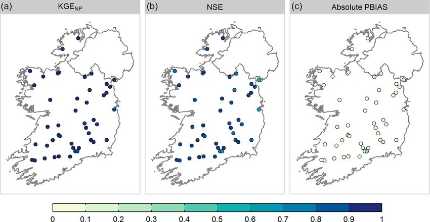
S. Donegan et al.: Conditioning ensemble streamflow prediction with the North Atlantic Oscillation                                                                           4163

Table 2. Summary statistics of eight catchment characteristics for Ireland and each NUTS III region. The median across n catchments is
given with the 5th and 95th percentile ranges in parentheses. Mean annual runoff (Q), precipitation (P ), and potential evaporation (PE) were
                                               ∗
calculated over calendar years 1992–2017. Fs is the long-term (calendar years 1992–2017) mean fraction of precipitation falling as snow.

  Region         n     Area (km2 )        Q (mm yr−1 )         P (mm yr−1 )         PE (mm yr−1 )              BFI (–)            RBI (–)             RR (–)             Fs (–)
  IE           46              412                  686                 1149                    565               0.59              0.19                0.62              0.02
                        (23, 2286)          (431, 1336)          (905, 1861)             (529, 580)       (0.34, 0.75)        (0.07, 0.5)        (0.5, 0.82)      (0.01, 0.02)
  B              6             180                  970                1484                     540               0.43               0.24               0.73              0.02
                        (94, 1279)          (569, 1371)        (1088, 1878)              (521, 551)        (0.3, 0.72)       (0.07, 0.55)       (0.59, 0.83)      (0.02, 0.02)
  E              8              290                 483                  926                    560               0.62               0.15              0.55               0.02
                          (7, 2193)          (385, 750)          (891, 1149)             (535, 574)       (0.44, 0.72)       (0.12, 0.45)        (0.47, 0.7)      (0.01, 0.02)
  MW           10              606                  697                1177                     571               0.58                0.2               0.64              0.02
                       (225, 1891)           (506, 900)        (1043, 1373)              (561, 585)       (0.45, 0.67)       (0.09, 0.36)        (0.5, 0.75)      (0.01, 0.02)
  M              6             360                  524                  986                    561              0.71                0.13               0.56              0.02
                        (38, 1147)           (440, 644)          (914, 1125)             (556, 566)        (0.53, 0.8)       (0.08, 0.26)       (0.52, 0.62)      (0.02, 0.02)
  SE             6             738                  644                 1085                    567               0.56               0.26               0.58              0.02
                       (145, 2397)          (473, 1044)          (981, 1325)             (545, 576)       (0.42, 0.66)       (0.19, 0.45)       (0.51, 0.85)      (0.02, 0.03)
  SW             6             603                  929                1581                     569               0.44                0.4              0.71               0.02
                       (269, 1206)          (668, 1500)        (1417, 1987)              (567, 574)       (0.34, 0.61)        (0.13, 0.5)        (0.65, 0.8)      (0.02, 0.02)
  W              4             308                 1046                1512                     552                0.6               0.18                0.7              0.01
                        (87, 1749)          (723, 1223)        (1198, 1695)              (545, 563)       (0.32, 0.75)        (0.1, 0.54)       (0.63, 0.76)      (0.01, 0.01)
∗ F was calculated following Berghuijs et al. (2014), where precipitation on days with an average temperature greater than or equal to 1 ◦ C was considered entirely rainfall, and
   s
precipitation on days with an average temperature below 1 ◦ C was considered entirely snowfall.

more complex model structures, which do not necessarily                                       subsequent modelling tasks. An approach of this nature is
lead to large improvements in skill (e.g. Bell et al., 2017).                                 beneficial as it allows for evaluation of the model’s ability to
GR4J is implemented in R via the open-source airGR pack-                                      accurately simulate catchment processes over two indepen-
age (v1.4.3.65; Coron et al., 2017, 2020).                                                    dent periods whilst maximising the information content of
   Model parameters were estimated using memetic algo-                                        the parameter set that is used to generate the ESP hindcast
rithms with local search chains (MA-LS-Chains; Bergmeir                                       time series. In all cases, 1992 was used as a warm-up period
et al., 2016; Molina et al., 2010). As ESP forecasts are                                      to initialise model states, and the full series (1993–2017) was
made throughout the year under varying conditions, the non-                                   simulated before calibration and testing to preserve the in-
parametric Kling–Gupta efficiency (KGENP ; Appendix A)                                        ternal dynamics and temporal stability of catchment stores.
was chosen as the objective function to optimise, as it has                                   Model performance was evaluated using KGENP , the Nash–
been shown to capture multiple parts of the hydrograph well                                   Sutcliffe efficiency (NSE; Nash and Sutcliffe, 1970), and the
(Pool et al., 2018). Parameter estimation was carried out in                                  percent bias (PBIAS; Gupta et al., 1999).
R using the Rmalschains package (v0.2-6; Bergmeir et al.,
2016, 2019) with the covariance matrix adaptation evolution                                   2.3     ESP study design
strategy (Hansen and Ostermeier, 2001) as the local search
method.                                                                                       2.3.1     Historical ESP
   Model calibration was performed following the proce-
dures recommended by Arsenault et al. (2018). A split-                                        Forecasts were initialised on the first day of each month fol-
sample test (Klemeš, 1986) was first used to assess model                                     lowing a 4-year model warm-up period to estimate initial
robustness. The available record was divided into two peri-                                   hydrological conditions. The first usable forecast date after
ods of equal length, denoted here as period 1 (P1; 1 January                                  model warm-up is, therefore, 1 January 1965. For each fore-
1993–2 July 2005) and period 2 (P2; 2 July 2005–31 Decem-                                     cast initialisation date, a 55-member ensemble m of stream-
ber 2017). Separate parameter sets were created using data                                    flow hindcasts was generated by forcing GR4J with corre-
from P1 and P2 in turn for calibration and validation (i.e. pa-                               sponding historic climate sequences (pairs of precipitation
rameters were calibrated on P1 and validated on P2 and vice                                   and potential evaporation) extracted from 1961–2016 out
versa). A third round of calibration was then performed using                                 to a 12-month lead time. Following Harrigan et al. (2018),
data from the complete period (CP; 1 January 1993–31 De-                                      streamflow at a given lead time is expressed as the mean daily
cember 2017). This parameter set was carried forward for all                                  streamflow from the forecast initialisation date to n days or

https://doi.org/10.5194/hess-25-4159-2021                                                                       Hydrol. Earth Syst. Sci., 25, 4159–4183, 2021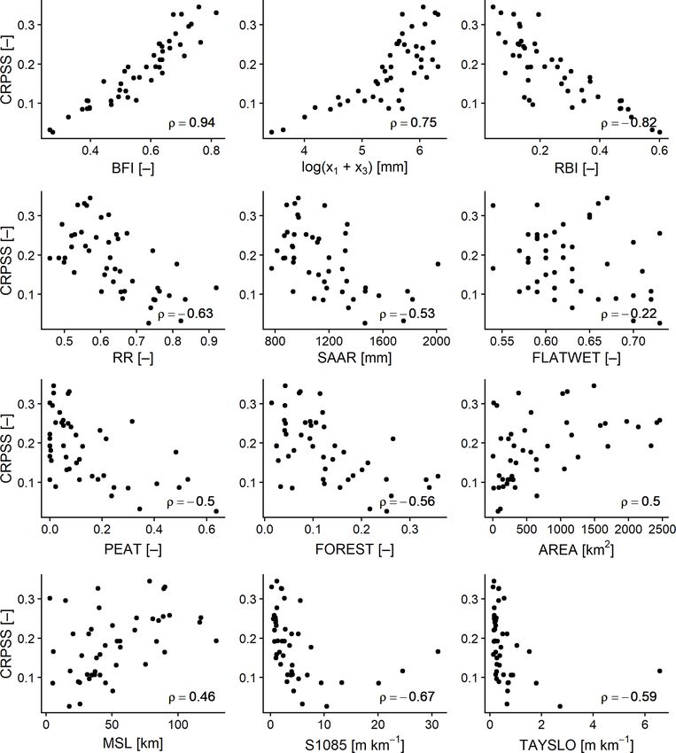
4164                 S. Donegan et al.: Conditioning ensemble streamflow prediction with the North Atlantic Oscillation

months ahead in time. For example, a January forecast with         served seasonal NAO approximated the mean adjusted sea-
a lead time of 1 month is the mean daily streamflow from           sonal NAO hindcast. This resulted in a 510-member ensem-
1 to 31 January, and a January forecast with a lead time of        ble of analogue date sequences, which were then used to ex-
2 months is the mean daily streamflow from 1 January to            tract corresponding precipitation and potential evaporation
28 February. Average flow values are used, particularly at         for input to the ESP method. The decision to construct ana-
monthly timescales because these are preferred by decision         logue seasons with months from different years was made
makers in many water sectors (Arnal et al., 2018). Hindcast        (a) to ensure that the range of possible values suggested by
time series were therefore temporally aggregated to provide        GloSea5 could be reproduced and (b) to avoid underestimat-
predictions of mean streamflow over lead times of 1 d to           ing extreme seasonal NAO values, which would sample ex-
12 months, resulting in 365 lead times per forecast (exclud-       clusively from DJF 2009–2010 if below −10 hPa (Stringer
ing leap days). In order to mimic operational conditions and       et al., 2020). Per hindcast member, 10 analogues were sam-
prevent artificial skill inflation (see Robertson et al., 2016),   pled to minimise non-NAO-related variability whilst keeping
we also employed leave-one-out cross-validation (L1OCV),           a consistent NAO signal across the sample. Conditioned ESP
whereby data from the forecast year were not used as in-           forecasts were only initialised on 1 December. A more de-
put to the model, as these would not be available in a real-       tailed description of the adjustment procedure and the selec-
time forecasting setting. For example, a forecast initialised      tion of the analogue date sequences is available in Stringer
on 1 January 1965 will use historic climate sequences of           et al. (2020).
365 d in length (1 January to 31 December) extracted from
1961–2016 but not 1965. ESP skill is evaluated over 52 ini-        2.4     Skill evaluation
tialisation years N (1965–2016) with 12 initialisation months
i (January to December). In total, 624 hindcasts were gen-         2.4.1    Hindcast overall performance
erated (N × i) with 34 320 individual ensemble members
(N × i × m), each at 365 lead times across 46 catchments,          We quantify the overall skill of the ESP method using the
resulting in a hindcast archive of more than 5.7×10⁸ stream-       continuous ranked probability score (CRPS; Hersbach, 2000)
flow values.                                                       and corresponding skill score (CRPSS; Appendix B). The
                                                                   CRPS is a recommended and widely used evaluation metric
2.3.2   Conditioned ESP                                            for ensemble hydrological forecasting (Pappenberger et al.,
                                                                   2015b) that penalises biased and unsharp forecasts (Wilks,
To investigate the potential for improving winter stream-          2019). To minimise the impact of hydrological model un-
flow predictability, we conditioned the ESP method using ad-       certainty on hindcast quality, we use modelled observations
justed NAO hindcasts from the Met Office’s Global Seasonal         derived from GR4J in place of direct streamflow data when
Forecasting System version 5 (GloSea5; MacLachlan et al.,          evaluating skill. This is common practice (e.g. Arnal et al.,
2015). GloSea5 is built around the high-resolution Hadley          2018; Harrigan et al., 2018; Wood and Lettenmaier, 2008;
Centre Global Environmental Model version 3 (HadGEM3),             Wood et al., 2016) as it isolates loss of skill to errors in initial
which integrates atmosphere, ocean, land, and sea-ice com-         conditions. Our reference forecast is constructed as the full-
ponents. HadGEM3 has an atmospheric resolution of 0.83◦            sample climatological distribution of modelled observations
longitude by 0.55◦ latitude, with 85 vertical levels and an        over 1965–2016 for the forecast period. This forecast was
ocean resolution of 0.25◦ in both latitude and longitude with      also created using L1OCV to account for streamflow persis-
75 vertical levels. Although GloSea5 has been shown to skil-       tence. In the case of the conditioned ESP, skill is calculated
fully predict the NAO (Scaife et al., 2014), several stud-         relative to both the probabilistic climatology benchmark and
ies have documented a signal-to-noise problem that limits          the full historical ESP ensemble. In all cases, the Ferro et al.
the usefulness of forecasts to drive hydrological models, as       (2008) ensemble size correction for CRPS is applied after
ensemble mean signals in NAO forecasts are anomalously             cross-validation to account for differences in the number of
weak (Eade et al., 2014; Scaife et al., 2014; Scaife and           ensemble members.
Smith, 2018). Focusing on the dynamical signals can correct
this by amplifying the ensemble mean (Baker et al., 2018),         2.4.2    Hindcast reliability
so adjusted hindcasts are used here following the method
of Stringer et al. (2020). For each DJF period over 1993–          Hindcast reliability was also assessed for low and high flows.
2016, we combined GloSea5 hindcasts initialised on 1, 9, and       Reliability refers to the overall agreement between the fore-
17 November, each with 17 ensemble members, to create a            cast probabilities and the observed frequencies. For each
51-member lagged ensemble of raw NAO predictions. Af-              catchment, initialisation month, and lead time, the probabil-
ter adjustment to remove the signal-to-noise discrepancy in        ity integral transform (PIT; Gneiting et al., 2007; Laio and
the raw ensemble, predicted monthly NAO values were used           Tamea, 2007) score was calculated for subsets of forecast–
to select 10 non-sequential DJF analogues (e.g. December           observation pairs falling within the lower and upper terciles
2007, January 1980, February 2011), where the mean ob-             of the corresponding modelled observations. The PIT score

Hydrol. Earth Syst. Sci., 25, 4159–4183, 2021                                        https://doi.org/10.5194/hess-25-4159-2021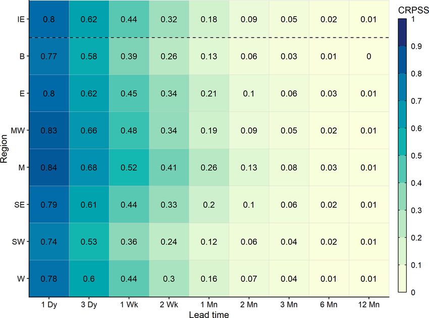
S. Donegan et al.: Conditioning ensemble streamflow prediction with the North Atlantic Oscillation                            4165

was derived from the PIT diagram following Renard et al.            this band range between 0.1 and 0.58 and for a 1-month lead
(2010). A forecast with a PIT score of 1 has perfect reliabil-      time between 0.03 and 0.4.
ity, whereas a forecast with a PIT score of 0 has the worst
reliability.                                                        3.2.2    Initialisation month

2.4.3    Hindcast discrimination                                    ESP skill varies with forecast initialisation month and time
                                                                    of year, with the highest and lowest skill scores dependent
Hindcasts were further assessed in terms of their ability to        on lead time (Fig. 4). For short to monthly lead times, skill
discriminate between events and non-events using the re-            scores are highest when forecasts are initialised in summer
ceiver operator characteristic (ROC; Mason and Graham,              (JJA), with July the most skilful initialisation month on aver-
1999) score. The ROC score is defined as the area under the         age, whereas skill tends to be lower during winter (DJF), with
ROC curve, which plots the probability of detection against         January and December exhibiting the lowest skill. At sea-
the probability of false detection for a given event and a range    sonal lead times, skill during autumn (SON) is comparable to
of probability levels (Demargne et al., 2010). A ROC score          that of summer, whilst the least skilful forecasts are produced
of 1 indicates that all ensemble members correctly predicted        in the spring months (MAM). As in Fig. 3, skill tends toward
the event in all years, whereas a ROC score of 0.5 indicates        zero as lead time increases, regardless of initialisation month.
a forecast with no discrimination. For each catchment, ini-         Although this decline in performance is less severe for sum-
tialisation month, and lead time, the ROC score was calcu-          mer than for other seasons, by a 12-month lead time, nearly
lated using the lower and upper terciles of the corresponding       all forecasts are less skilful than climatology. Despite this,
modelled observations as thresholds. Hence, the ROC score           several catchments have above (below) average skill scores,
should be interpreted as a measure of how well ESP can fore-        with some performing notably better (worse) across different
cast the occurrence of low- and high-flow events and can            lead times and initialisation months. For example, ESP fore-
thus be regarded as an indicator of potential usefulness. We        casts initialised in July with a 1-month lead have moderate
use a slightly stricter skill threshold of 0.6, so that forecasts   skill on average (CRPSS = 0.34), but seven catchments have
are only considered skilful if they are better than guesswork.      high skill (CRPSS ≥ 0.5), with a maximum CRPSS of 0.68
Both the CRPSS and ROC score were calculated in R using             for the Erkina (ID 15005). Conversely, 14 catchments have
the easyVerification package (v0.4.4; MeteoSwiss, 2017).            low skill (CRPSS ≤ 0.25), with a minimum of −0.03 for the
                                                                    Newport (ID 32012).

3     Results                                                       3.3     Spatial distribution of ESP skill

3.1     Hydrological model performance                              3.3.1    NUTS III regions

GR4J performed well for our catchment sample (Fig. 2). The          Mean ESP skill across all initialisation months is shown
median (5th and 95th percentile) value of KGENP is 0.95             in Fig. 5 for Ireland and each of the seven NUTS III re-
(0.88, 0.97) for calibration over P1, P2, and CP. Median val-       gions. The Midlands, Mid-West, and East are the most skil-
idation scores of 0.91 (0.84, 0.96) were achieved during test-      ful regions, followed by the South-East, West, and Border
ing on both P1 and P2. Median NSE for calibration over CP           regions. The South-West is the least skilful region on av-
is 0.88 (0.69, 0.93), and median PBIAS is 0.04 % (−0.13 %,          erage, with the lowest CRPSS values for all sampled lead
0.14 %). Performance metrics and calibrated parameter val-          times. Regional variations in skill are less pronounced at
ues for individual catchments over CP are given in Table S1.        shorter lead times but become more apparent as lead time
                                                                    increases. For example, at a 1-month lead time, the Mid-
3.2     Timing of ESP skill                                         lands (CRPSS = 0.26) is twice as skilful as the Border
                                                                    (CRPSS = 0.13) and South-West (CRPSS = 0.12). All re-
3.2.1    Lead time                                                  gions are, on average, skilful out to a 1-month lead time,
                                                                    but the Midlands is the only region that is moderately skil-
Mean ESP skill declines rapidly as a function of lead time,         ful (CRPSS ≥ 0.25). The Midlands remains the most skilful
across all catchments and initialisation months (Fig. 3). Mean      region beyond 1-month, though the level of skill is generally
CRPSS values for short (1 d) to extended (2-week) lead times        quite low for all regions by this point. The regional variations
range from 0.8 to 0.32 and for monthly (1- and 2-month), sea-       observed in Fig. 5 are partly explained by the relationship be-
sonal (3-month), and annual lead times from 0.18, 0.09, and         tween catchment characteristics and ESP skill (Sect. 3.4) as
0.05 to 0.01, respectively. However, the rate at which skill de-    the pattern is broadly consistent with differences in catch-
cays across catchments varies, with considerable differences        ment storage capacity and wetness. For instance, the Mid-
around the mean shown by the 5th and 95th percentile bands.         lands has a high median BFI of 0.71, a low median RBI
For example, for a 2-week lead time, CRPSS values within            of 0.13, and a low median SAAR of 939 mm, whereas the

https://doi.org/10.5194/hess-25-4159-2021                                         Hydrol. Earth Syst. Sci., 25, 4159–4183, 2021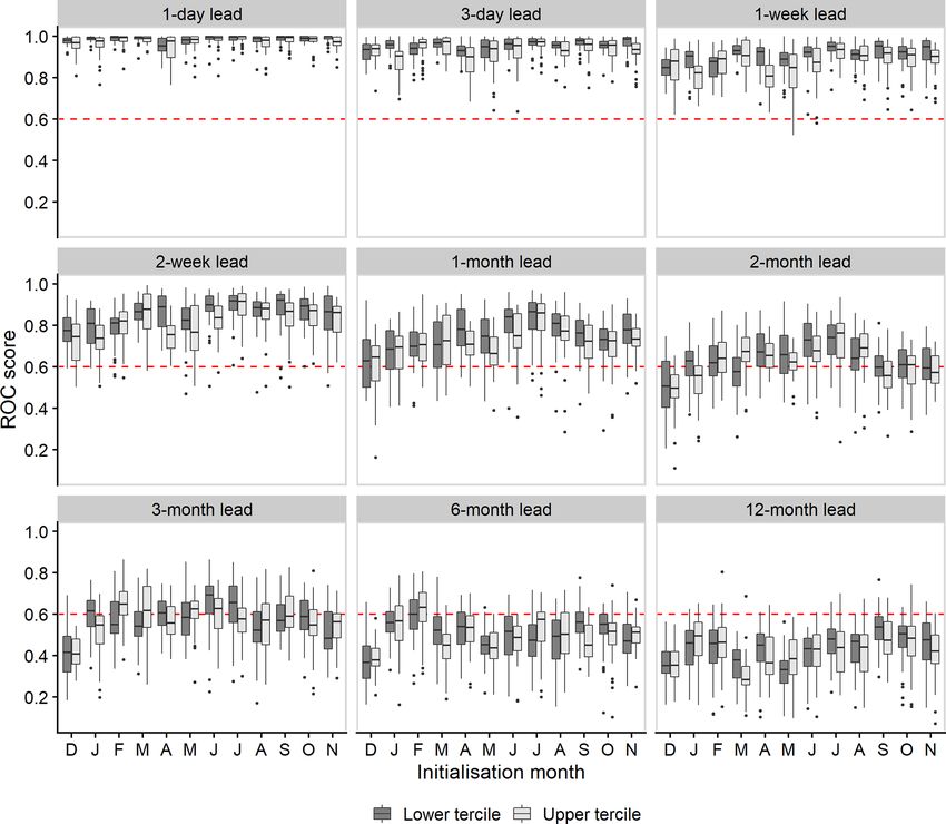
4166                  S. Donegan et al.: Conditioning ensemble streamflow prediction with the North Atlantic Oscillation

Figure 2. GR4J model performance over the complete period (1993–2017) as measured by KGENP (a), NSE (b), and absolute PBIAS (c).

Figure 3. Mean ESP CRPSS values across all 46 study catchments, 12 forecast initialisation months, and all 365 lead times, with short and
extended lead times shown inset for readability. Variations in skill scores across all catchments at each lead time are given by the 5th and
95th percentile ensemble range.

South-West has a low median BFI of 0.44, a high median RBI              for several catchments at different times of the year, even if
of 0.4, and a high median SAAR of 1407 mm. Differences                  average skill for the region as a whole tends to be low. For
in regional hydroclimate properties therefore contribute to             example, whilst the South-West is the least skilful region at a
differences in regional skill as forecasts perform better in            1-month lead time, with an average CRPSS of 0.12, forecasts
the baseflow-dominated catchments of the Midlands than the              with above-average skill are possible in several catchments
flashy, wetter catchments of the South-West.                            in the region in June, such as the Blackwater (ID 18003;
                                                                        CRPSS = 0.25) and the Laune (ID 22035; CRPSS = 0.23).
3.3.2   Catchment scale
                                                                        3.4    Relationship with catchment characteristics
Notable subregional heterogeneity emerges when examining
skill scores for individual forecasts at the catchment scale            Figure 7 shows the relationship between ESP skill, as
(Fig. 6). This heterogeneity is more noticeable at monthly              represented by the average 1-month CRPSS, and several
to seasonal lead times, where skilful forecasts are possible            PCDs for each of the 46 study catchments using the non-

Hydrol. Earth Syst. Sci., 25, 4159–4183, 2021                                             https://doi.org/10.5194/hess-25-4159-2021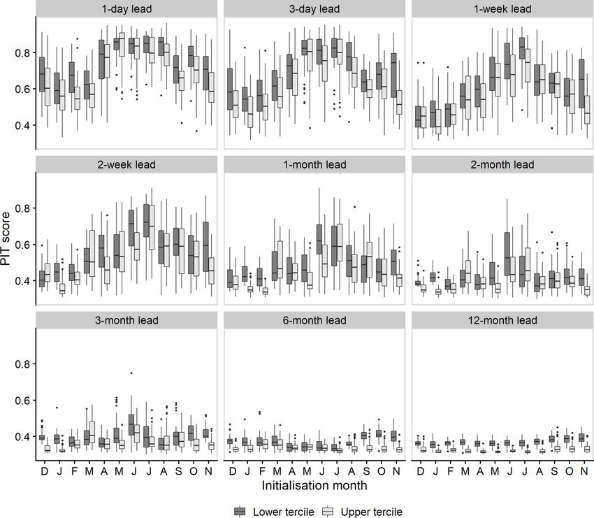
S. Donegan et al.: Conditioning ensemble streamflow prediction with the North Atlantic Oscillation                                       4167

Figure 4. As in Fig. 3 but for each forecast initialisation month. Data from Fig. 3 are included in the background of each panel for reference.

parametric Spearman rank correlation coefficient (ρ). ESP                 catchments are more likely to be those with lower storage
skill is closely linked with catchment storage properties and             and flashier regimes in which ESP has already been shown
responsiveness. There are strong positive correlations be-                to perform poorly. Poor skill in these catchments is likely
tween modelled storage capacity (x1 +x3 ) and BFI (ρ = 0.79)              a combination of high precipitation and low permeability,
and between ESP skill and BFI (ρ = 0.94). There is also a                 which leads to more variable hydrological conditions as rain-
strong positive correlation between ESP skill and modelled                fall events propagate to streamflow quickly. Finally, there are
storage capacity (ρ = 0.75). Conversely, there is a strong neg-           moderate negative correlations between ESP skill and S1085
ative correlation between ESP skill and the RBI (ρ = −0.82)               (ρ = −0.67) and TAYSLO (ρ = −0.59), indicating that fore-
and a moderate negative correlation between ESP skill and                 casts are less skilful in catchments with steeper gradients.
the RR (ρ = −0.63). All of these correlations are statisti-               Although these results are based on the 1-month CRPSS av-
cally significant (p ≤ 0.05). In general, ESP skill tends to be           eraged across all initialisation months, similar results are ob-
higher for slower responding catchments with greater stor-                served for a variety of different months and lead times (not
age capacity and lower for faster responding, flashy catch-               shown).
ments with poor infiltration. ESP skill is also positively cor-
related with catchment area (ρ = 0.5) and main-stream length              3.5   Reliability of low- and high-flow forecasts
(ρ = 0.46), indicating a tendency for the method to perform
better in larger catchments with longer streams. Negative cor-            ESP is capable of producing reliable forecasts of both low
relations exist between ESP skill and PCDs related to catch-              (lower tercile) and high (upper tercile) flows (Fig. 8). How-
ment wetness (SAAR, FLATWET, and PEAT), though these                      ever, the level of reliability is dependent on both lead time
PCDs also exhibit negative correlations with BFI and posi-                and initialisation month. Reliability decreases as lead time
tive correlations with RBI and RR, highlighting that wetter               increases, though the rate at which this occurs is not uniform
                                                                          across all initialisation months. Furthermore, there is con-

https://doi.org/10.5194/hess-25-4159-2021                                               Hydrol. Earth Syst. Sci., 25, 4159–4183, 2021
4168 S. Donegan et al.: Conditioning ensemble streamflow prediction with the North Atlantic Oscillation
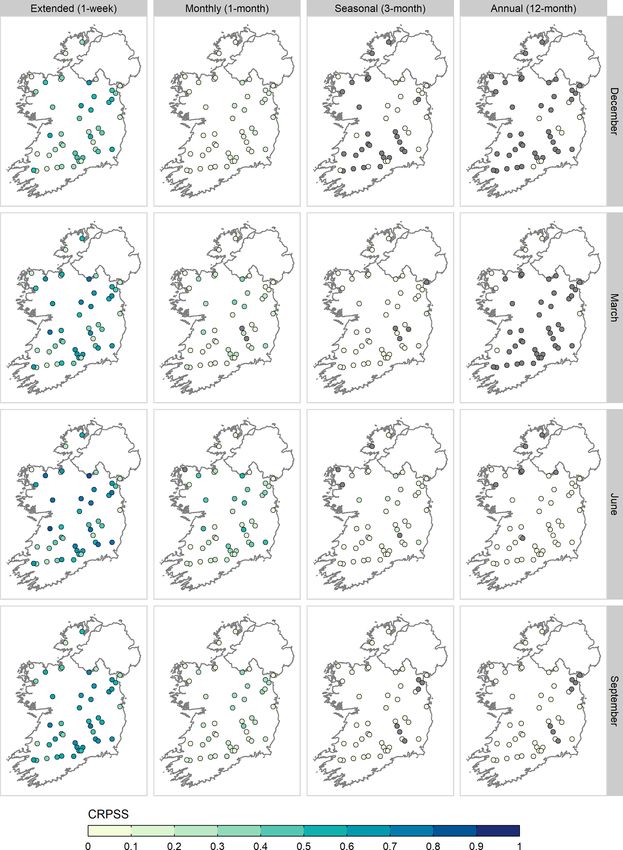
Figure 5. CRPSS values for Ireland (IE) and seven NUTS III regions (B, E, MW, M, SE, SW, and W) averaged across all initialisation
months for a selection of lead times: short (1 and 3 d), extended (1- and 2-week), monthly (1- and 2-month), seasonal (3- and 6-month) and
annual (12-month).
siderable inter-catchment variability for both low- and high- catchments and initialisation dates, with little or no skill at
flow forecasts. This latter point is perhaps most pronounced lead times of 6 and 12 months across the majority of the
at short to extended lead times but is also evident at longer catchment sample. Some seasonality in ROC skill is appar-
leads (e.g. 1- and 2-month forecasts initialised in June and ent, particularly at monthly lead times, where ESP can more
July), where some catchments return much higher than aver- skilfully discriminate between events and non-events in sum-
age PIT scores. Reliability tends to be highest when forecasts mer than other seasons. Discrimination is more skilful for
are initialised in summer and lowest when initialised in win- low-flow events than high-flow events.
ter, with the smallest and largest reductions in PIT scores also
evident for these seasons as lead time increases. Across all 3.7 Improvements in winter skill
lead times and initialisation months, reliability is, on aver-
age, higher for low-flow forecasts than high-flow forecasts. The overall skill (CRPSS) of NAO-conditioned ESP is com-
Although the PIT score decays with lead time, unlike the pared with that of historical ESP in Fig. 10. Whilst historical
CRPSS it does not tend toward zero and instead has a lower ESP is skilful in the majority of catchments at a 1-month
bound of around 0.3. Hence, somewhat reliable forecasts of lead time, there is a dramatic reduction in both the magni-
both low and high flows are still possible at annual lead times tude of skill and the number of catchments for which skilful
even when overall skill (CRPSS) is poor. forecasts can be made at 2- and 3-month lead times. NAO-
conditioned ESP outperforms historical ESP relative to the
climatology benchmark in all but one catchment at a 1-month
3.6 Discrimination between events and non-events
lead time, though these improvements are generally modest,
with a median (5th and 95th percentile) difference in CRPSS
In general, ESP is skilful at forecasting the occurrence of of 0.04 (0.01, 0.07). At a lead time of 2 months, NAO-
both low-flow (lower tercile) and high-flow (upper tercile) conditioned ESP remains skilful against climatology in 98 %
events up to 1 month ahead in the majority of catchments and of catchments, compared to historical ESP which is only skil-
for all initialisation months (Fig. 9). Discrimination for both ful in 37 % of catchments. The value of the NAO-conditioned
event types is also possible at lead times of 2 and 3 months, ESP is more evident at a 3-month lead time, where skilful
though to a lesser extent. These results highlight that ESP forecasts are still possible for several catchments in the Bor-
still has utility at longer lead times, even when overall per- der and western regions, when historical ESP exhibits little
formance as measured by the CRPSS is poor. However, this or no skill across the majority of the sample.
utility seldom extends beyond 3 months, except for specific
Hydrol. Earth Syst. Sci., 25, 4159–4183, 2021 https://doi.org/10.5194/hess-25-4159-2021S. Donegan et al.: Conditioning ensemble streamflow prediction with the North Atlantic Oscillation 4169 Figure 6. ESP skill for individual forecasts made at the 46 catchments for four sample lead times (columns) and 4 initialisation months (rows). Catchments with negative skill (CRPSS < 0) are greyed out. Over the three lead times examined here, the greatest im- RR values of 1570 mm and 0.79, respectively, although it is provements are found for wet, fast-responding catchments not as flashy (RBI = 0.18). NAO-conditioned forecasts gen- with low baseflow contribution. For example, two of the best- erally perform the worst in slowly responding catchments performing catchments for NAO-conditioned ESP are the with high storage capacity. At a lead time of 3 months, neg- Owenea (ID 38001) and the Fern (ID 39009). The Owenea ative skill is observed in several catchments in the East and has a BFI of 0.27, the lowest in the sample, with high SAAR South-East, though these values can still be defined within (1753 mm), RR (0.82), and RBI (0.58) values. The Fern has the bounds of what Bennett et al. (2017) refer to as “neu- a below-average BFI of 0.47, with similarly high SAAR and tral skill” (±0.05 CRPSS) and hence do not represent a sig- https://doi.org/10.5194/hess-25-4159-2021 Hydrol. Earth Syst. Sci., 25, 4159–4183, 2021
4170                  S. Donegan et al.: Conditioning ensemble streamflow prediction with the North Atlantic Oscillation

Figure 7. Relationship between 1-month ESP skill (CRPSS) and selected catchment descriptors.

nificant departure from the performance of historical ESP.            observed have high baseflow contribution and long recession
These differences in performance can be explained by the              times. Hence, hydrological response is controlled predomi-
relative contribution of initial conditions and meteorological        nately by the slow release of water from reservoirs, and initial
forcing to ESP skill. In the flashy catchments where NAO-             conditions act as the primary source of skill. The combina-
conditioned ESP performs well, meteorological conditions              tion of initial conditions and subsampled climate information
are the dominant control on skill as rainfall events propagate        grants modest improvements in skill in these catchments up
to streamflow at a faster rate, and memory of initial condi-          to a 1-month lead time. However, at longer lead times, im-
tions is lost quickly. It is also worth noting that in these catch-   proved atmospheric representation alone cannot compensate
ments skill generally increases with lead time. This is likely        for divergences from the initial state. Skill deteriorates as a
due to the fact that the underlying NAO signal is not as strong       result, eventually becoming negative.
over shorter averaging periods due to the noise of the individ-          In addition to the CRPSS, both the PIT score and the ROC
ual weather systems. Moreover, only the seasonal mean NAO             score were calculated for NAO-conditioned ESP. Figure 11
is rescaled to account for the signal-to-noise problem when           shows the difference between PIT scores calculated for his-
adjusting hindcasts, so skill is only present at the longer 3-        torical ESP and NAO-conditioned ESP at lead times of 1,
month lead time. For example, at a 3-month lead time, NAO-            2, and 3 months. Conditioning ESP with the NAO increases
conditioned ESP improves forecast skill by ∼ 18 % over his-           the reliability of low-flow forecasts in all catchments at a 1-
torical ESP in both the Owenea and Fern, whereas gains of             month lead time. Some catchments experience a reduction in
7 % and 12 % are observed for 1- and 2-month lead times,              low-flow reliability at a 2-month lead time, whereas at a 3-
respectively. Conversely, catchments where negative skill is          month lead time, low-flow reliability is observed to increase

Hydrol. Earth Syst. Sci., 25, 4159–4183, 2021                                          https://doi.org/10.5194/hess-25-4159-2021
S. Donegan et al.: Conditioning ensemble streamflow prediction with the North Atlantic Oscillation                                    4171

Figure 8. Distribution of PIT score values across all 46 study catchments for each initialisation month and the same selection of lead times
as in Fig. 5.

in almost all catchments. High-flow reliability increases in            the skill threshold. Although this is also observed for histor-
some catchments at a 1-month lead time but then decreases               ical ESP, it is less frequent.
in almost all catchments at lead times of 2 and 3 months.                  Changes in reliability are generally consistent with im-
At these longer lead times, increases in high-flow reliabil-            provements in skill (CRPSS) and discrimination (ROC). Im-
ity tend to be restricted to flashy catchments (e.g. Owenea),           proved low-flow reliability allows NAO-conditioned ESP to
where NAO-conditioned ESP has already been shown to per-                better distinguish between low-flow events and non-events.
form well in terms of CRPSS.                                            The reductions in low-flow reliability in some catchments
   ROC scores for individual catchments and the full range              at a 2-month lead time are also consistent with NAO-
of lead times are presented in Fig. 12. On average, NAO-                conditioned ESP “losing” ROC skill before later regaining
conditioned ESP extends the lead time over which discrim-               it (Fig. 12). Increases in high-flow reliability at a 3-month
ination between events and non-events is possible by 141 %              lead time in flashy catchments correspond with the greatest
for low flows (37 to 89 d) and 170 % for high flows (33 to              increases in CRPSS from NAO-conditioned ESP. In these
89 d). These are considerable improvements over historical              catchments, where streamflow variability is greater and the
ESP, which failed to meet the skill threshold in most catch-            NAO is most influential, improved reliability and sharpness
ments at longer lead times. For example, skilful discrimina-            lead to better overall skill at longer lead times.
tion of low-flow events is possible in 78 % of catchments at a
3-month lead time when using NAO-conditioned ESP com-
pared to only 11 % of catchments when using historical ESP.             4     Discussion
This makes NAO-conditioned ESP particularly effective at
forecasting dry winters, which can be critical for water re-            4.1    When is ESP skilful?
sources management. It is worth noting that in many catch-
                                                                        For short lead times (1–3 d), ESP forecasts are on average
ments NAO-conditioned ESP can “lose” skill before later re-
                                                                        highly skilful (CRPSS ≥ 0.5) and for extended lead times
gaining it, with the ROC score falling only marginally below
                                                                        (1–2 weeks) moderately skilful (CRPSS ≥ 0.25). Mean ESP
                                                                        skill decays rapidly with lead time. Hence, forecast skill for

https://doi.org/10.5194/hess-25-4159-2021                                             Hydrol. Earth Syst. Sci., 25, 4159–4183, 2021
4172 S. Donegan et al.: Conditioning ensemble streamflow prediction with the North Atlantic Oscillation Figure 9. As in Fig. 8 but for the ROC score. The red line denotes the stricter skill threshold of 0.6. monthly, seasonal, and annual lead times is on average much ful when initialised in winter. This is again consistent with lower. This is because ESP relies on the long-term “memory” previous research, with higher predictability during dry sea- of the hydrological system. The cumulative effect of distinct sons for forecasting methods that rely on hydrological mem- meteorological forcing causes a divergence from the initial ory reported for the UK (Harrigan et al., 2018), Switzerland state that grows with time. Thus, ESP suffers at longer lead (Staudinger and Seibert, 2014), China (Yang et al., 2014), times as there is little or no persistence of initial hydrologi- and parts of the Amazon Basin (Paiva et al., 2012). This cal conditions. Over longer periods, we find that ESP is most likely stems from a reduction in the direct contribution of skilful out to a month ahead (CRPSS = 0.18) but that some precipitation to streamflow (Li et al., 2009; Mo and Letten- predictability (CRPSS > 0.05) is possible up to 3 months in maier, 2014; Wood and Lettenmaier, 2008), which reduces advance. This rapid decline in forecast skill is consistent with variability and allows initial conditions to persist for longer. findings from several other benchmarking experiments, in- In winter, lower evaporation rates lead to more effective rain- cluding Harrigan et al. (2018) and Girons Lopez et al. (2021), fall, which “disrupts” the initial state and limits the skill of who noted a similar deterioration in ESP skill in the UK ESP forecasts. This is particularly noticeable in flashy catch- and Sweden, respectively. Pechlivanidis et al. (2020) also ments with a low baseflow contribution, where the hydrolog- reported a decline in seasonal streamflow forecasting skill ical response is driven predominately by rainfall. Under such with increasing lead time across Europe. Persistence fore- conditions, rainfall events propagate to streamflow at a much casts, which also rely on hydrological memory as their main faster rate, and memory of initial conditions is lost quickly. source of skill, have shown comparable results. For example, At longer lead times, ESP is least skilful when initialised both Svensson (2016) and Foran Quinn et al. (2021) noted a in spring. Both Harrigan et al. (2018) and Svensson (2016) reduction in the number of usable persistence forecasts in the also found lower longer range skill for forecasts initialised in UK and Ireland, respectively, when moving from a 1-month spring in the UK. The former attributed this to the transition forecast horizon to a 3-month forecast horizon. from wet conditions with small soil moisture deficits to dry ESP skill is also highly dependent on initialisation month. conditions with large soil moisture deficits. Given that Ire- On average, at short to extended lead times (1 d to 2 weeks), land shares a similar precipitation regime to the UK and that ESP is most skilful when initialised in summer and least skil- ESP skill is negatively impacted by high rainfall variability Hydrol. Earth Syst. Sci., 25, 4159–4183, 2021 https://doi.org/10.5194/hess-25-4159-2021
S. Donegan et al.: Conditioning ensemble streamflow prediction with the North Atlantic Oscillation                             4173

Figure 10. CRPSS values for historical ESP (a, d, g), NAO-conditioned ESP (b, e, h), and the improvement made by NAO-conditioned ESP
over historical ESP (c, f, i), at lead times of 1, 2, and 3 months (rows). Catchments with negative skill (CRPSS < 0) are greyed out.

across the forecast period (Harrigan et al., 2018), this is also     ity and hence greater skill due to their long memory. Both
a plausible explanation for the results observed here.               the Border and the West are poorly drained regions, with
                                                                     the former characterised by unproductive bedrock aquifers.
4.2   Where is ESP skilful?                                          This partly explains the low storage capacity of catchments in
                                                                     these regions, which have quick hydrological response times
ESP is most skilful in the Midlands and least skilful in the         and poor persistence of initial conditions, resulting in lower
Border and South-West. The Midlands is a lowland karst re-           ESP skill. Similar patterns were noted for persistence fore-
gion, which is underlain by permeable Carboniferous lime-            casts (Foran Quinn et al., 2021).
stone, characterised by several locally and regionally impor-
tant aquifers. Given that soils in this region are also well
drained, catchments located here have higher storage capac-

https://doi.org/10.5194/hess-25-4159-2021                                         Hydrol. Earth Syst. Sci., 25, 4159–4183, 2021
4174 S. Donegan et al.: Conditioning ensemble streamflow prediction with the North Atlantic Oscillation
Figure 11. Difference in PIT score values between NAO-conditioned ESP and historical ESP at lead times of 1, 2, and 3 months. Negative
values indicate a reduction in reliability, whereas positive values indicate an increase in reliability over historical ESP.
4.3 Why is ESP skilful? which can lead to temporal streamflow dependence for up to
a season ahead (Chiverton et al., 2015).
ESP skill displays a strong relationship with modelled catch- 4.4 Potential for operationalising ESP in Ireland
ment storage capacity and catchment BFI values, with higher
skill scores returned for catchments with greater storage. Our benchmarking results establish that ESP, in its tradi-
We conclude that storage capacity is primarily responsible tional formulation, is skilful in a number of different scenar-
for modulating ESP skill. High BFI catchments have flow ios, sometimes up to several months in advance. We recom-
regimes dominated by slowly released groundwater (Chiver- mend that ESP be used operationally in Ireland, similar to the
ton et al., 2015) and are characterised by longer response HOUK (Prudhomme et al., 2017). Skilful streamflow fore-
times and lower streamflow variability (Sear et al., 1999; casts at short to extended lead times could prove beneficial
Broderick et al., 2016). This is conducive to greater per- for water resources management, particularly in areas such
sistence of initial conditions, with water storage in the soil as Dublin where water supply systems have been operating
creating a memory effect whereby anomalous conditions can close to capacity and face challenges of supply during dry
take weeks or months to wane (Ghannam et al., 2014; Harri- periods. Given that the predictability of summer rainfall is
gan et al., 2018; Li et al., 2009). The role played by storage notoriously difficult over northern Europe (Weisheimer and
capacity is perhaps best illustrated by the fact that ESP skill Palmer, 2014), the true utility of ESP may lie in its ability to
decays at a much slower rate in catchments with high BFI, es- leverage initial hydrological conditions, particularly in high-
pecially during summer when streamflow is derived primar- storage catchments, to skilfully predict streamflow up to a
ily from stored sources. For example, ESP is moderately skil- season ahead during dry months. Operationally, skill could
ful (CRPSS ≥ 0.25) out to a 2-month lead time for the Inny be extended further by initialising forecasts more than once
(ID 26021; BFI = 0.82) when initialised in July but shows a month (e.g. Girons Lopez et al., 2021). As ESP has also
adequate (non-neutral) performance relative to climatology been shown to accurately forecast the occurrence of low- and
(CRPSS > 0.05) up to 4 months ahead. Moreover, whilst ESP high-flow events in many catchments up to at least a month
tends to perform worse outside of summer months, catch- in advance, it may also have practical relevance for decision
ments with relatively high SAAR but also high BFI yield makers where it can act as an aid in the management of hy-
above-average skill scores in winter, spring, and autumn. In drologic extremes.
the Slaney (ID 12001; BFI = 0.67; SAAR = 1167 mm), skil- In the absence of skilful atmospheric forecasts or im-
ful forecasts are possible up to almost a year ahead in Jan- proved hydrological process representation, historical ESP
uary and February and up to 3–6 months ahead in spring and provides a lower limit of streamflow forecasting skill (Har-
autumn. This likely stems from the delayed release of pre- rigan et al., 2018). However, we show that it is possible to
cipitation from groundwater stores (van Dijk et al., 2013), improve ESP skill during winter by conditioning the method
Hydrol. Earth Syst. Sci., 25, 4159–4183, 2021 https://doi.org/10.5194/hess-25-4159-2021You can also read