First assessment of the earth heat inventory within CMIP5 historical simulations - Earth System Dynamics
←
→
Page content transcription
If your browser does not render page correctly, please read the page content below
Earth Syst. Dynam., 12, 581–600, 2021
https://doi.org/10.5194/esd-12-581-2021
© Author(s) 2021. This work is distributed under
the Creative Commons Attribution 4.0 License.

                    First assessment of the earth heat inventory
                         within CMIP5 historical simulations
            Francisco José Cuesta-Valero1,2 , Almudena García-García1,3 , Hugo Beltrami1 , and Joel Finnis4
              1 Climate & Atmospheric
                                    Sciences Institute, St. Francis Xavier University, Antigonish, NS, Canada
              2 Environmental
                            Sciences Program, Memorial University of Newfoundland, St. John’s, NL, Canada
          3 Department of Remote Sensing, Helmholtz Centre for Environmental Research-UFZ, Leipzig, Germany
                4 Department of Geography, Memorial University of Newfoundland, St. John’s, NL, Canada

                                       Correspondence: Hugo Beltrami (hugo@stfx.ca)

                                 Received: 3 December 2020 – Discussion started: 28 December 2020
                                         Accepted: 1 April 2021 – Published: 10 May 2021

       Abstract. The energy imbalance at the top of the atmosphere over the last century has caused an accumulation
       of heat within the ocean, the continental subsurface, the atmosphere and the cryosphere. Although ∼ 90 % of
       the energy gained by the climate system has been stored in the ocean, the other components of the Earth heat
       inventory cannot be neglected due to their influence on associated climate processes dependent on heat storage,
       such as sea level rise and permafrost stability. However, there has not been a comprehensive assessment of
       the heat inventory within global climate simulations yet. Here, we explore the ability of 30 advanced general
       circulation models (GCMs) from the fifth phase of the Coupled Model Intercomparison Project (CMIP5) to
       simulate the distribution of heat within the Earth’s energy reservoirs for the period 1972–2005 of the Common
       Era. CMIP5 GCMs simulate an average heat storage of 247 ± 172 ZJ (96 ± 4 % of total heat content) in the
       ocean, 5 ± 9 ZJ (2 ± 3 %) in the continental subsurface, 2 ± 3 ZJ (1 ± 1 %) in the cryosphere and 2 ± 2 ZJ (1 ±
       1 %) in the atmosphere. However, the CMIP5 ensemble overestimates the ocean heat content by 83 ZJ and
       underestimates the continental heat storage by 9 ZJ and the cryosphere heat content by 5 ZJ, in comparison with
       recent observations. The representation of terrestrial ice masses and the continental subsurface, as well as the
       response of each model to the external forcing, should be improved in order to obtain better representations of the
       Earth heat inventory and the partition of heat among climate subsystems in global transient climate simulations.

1   Introduction                                                   society is strongly dependent on the partition of heat among
                                                                   all climate components.
                                                                      The evolution of ocean heat content determines the ther-
Sustained net radiative imbalance at the top of the atmo-          mosteric component of sea level rise (Church et al., 2011;
sphere is increasing the heat stored within the climate subsys-    Kuhlbrodt and Gregory, 2012; Levitus et al., 2012), affects
tems – the ocean, the continental subsurface, the atmosphere       the total precipitation and intensity of hurricanes (Mainelli
and the cryosphere (Hansen et al., 2011; von Schuckmann            et al., 2008; Wada and Chan, 2008; Lin et al., 2013; Tren-
et al., 2020). The ocean is the largest component of the Earth     berth et al., 2018), and influences regional cyclonic activity
heat inventory (EHI), accounting for around 90 % of the total      (Bhowmick et al., 2016). The increase in ground heat content
heat in the climate system (Rhein et al., 2013; Gleckler et al.,   leads to the warming of the continental subsurface and to per-
2016; von Schuckmann et al., 2020). Nonetheless, it is im-         mafrost thawing in the Northern Hemisphere (Koven et al.,
perative to measure the distribution of heat storage within the    2013; Cuesta-Valero et al., 2016; McGuire et al., 2018; Bisk-
four components of the climate system, since the evolution of      aborn et al., 2019; Hock et al., 2019; Meredith et al., 2019;
several physical processes critical to understanding climate       Soong et al., 2020). Thus, the increase in continental heat
change and quantifying future impacts of climate change on

Published by Copernicus Publications on behalf of the European Geosciences Union.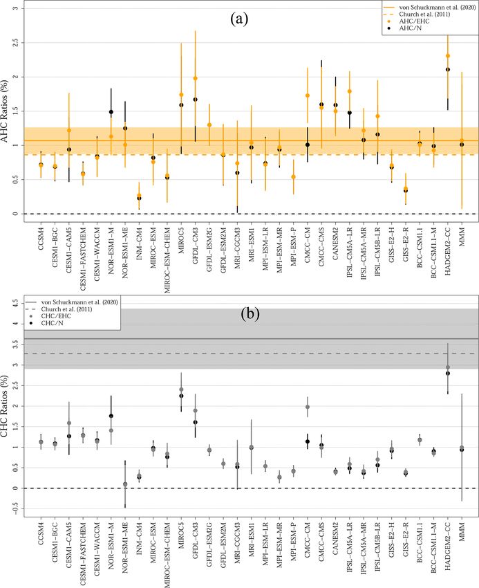
582                                                          F. J. Cuesta-Valero et al.: Earth heat inventory in CMIP5 models

storage threatens the stability of the global soil carbon pool,    tions, nevertheless, do not simulate other aspects of the Earth
potentially facilitating the release of large amounts of green-    heat inventory successfully. CMIP5 simulations are unable
house gasses from the decomposition of soil organic mat-           to accurately represent heat storage within the continental
ter in northern soils (Koven et al., 2011; MacDougall et al.,      subsurface over the second half of the 20th century (Cuesta-
2012; Schädel et al., 2014; Schuur et al., 2015; Hicks Pries       Valero et al., 2016), and many do not conserve atmospheric
et al., 2017; McGuire et al., 2018). Melting of ice sheets in      water (Liepert and Lo, 2013) or subsurface water (Krakauer
Greenland and Antarctica as well as glacier degradation at         et al., 2013; Trenberth et al., 2016) and do not conserve the
all latitudes contribute to sea level rise (Jacob et al., 2012;    total heat in the system (Hobbs et al., 2016). Furthermore,
Hanna et al., 2013; Vaughan et al., 2013; Dutton et al., 2015;     there has not yet been an assessment of the ability of CMIP5
Bamber et al., 2018; King et al., 2018; Rignot et al., 2019;       GCMs to reproduce heat storage within the atmosphere and
Hock et al., 2019; Oppenheimer et al., 2019; Meredith et al.,      the cryosphere, despite their impact on a variety of phenom-
2019; Zemp et al., 2019) and, together with changes in the         ena of critical interest to both society and the scientific com-
extension and volume of sea ice, may disturb deep water for-       munity.
mation zones and alter ocean circulation and large-scale heat         Here, we assess the ability of 30 CMIP5 GCM “Historical”
distribution (Hu et al., 2013; Jahn and Holland, 2013; Ferrari     simulations to reproduce the Earth heat inventory and the
et al., 2014; Smeed et al., 2018; Collins et al., 2019). The       partition of heat within the ocean, continental subsurface, at-
evolution of the atmosphere heat content constrains the pro-       mosphere and cryosphere. Results are compared with obser-
jected change in total global precipitation due to atmospheric     vations for the period 1972–2005 of the Common Era (CE).
warming (Pendergrass and Hartmann, 2014a; Hegerl et al.,           Our analysis reveals the importance of the simulated terres-
2015), and the additional moisture in a warmer atmosphere          trial ice masses and the represented continental subsurface
increases the frequency of extreme precipitation events (Pen-      volume for achieving a realistic distribution of the total Earth
dergrass and Hartmann, 2014b). The intensity of cyclones           heat content within GCM simulations, and it reinforces the
and hurricanes is also expected to increase in the future due      need to reduce the spread in model responses to external forc-
to the higher energy available in the atmosphere (Pan et al.,      ing.
2017).
   Therefore, the partition of heat within these subsystems
has long-term impacts on society, as the heat content of each      2   Data and methods
subsystem is related to processes altering near-surface condi-
tions. Higher surface temperatures together with changes in        A total of 30 Historical simulations performed with ad-
precipitation regimes and sea level rise threaten global food      vanced general circulation models were retrieved from
security (Lloyd et al., 2011; Rosenzweig et al., 2014; Phalkey     the fifth phase of the Coupled Model Intercomparison
et al., 2015; Campbell et al., 2016) and may result in an in-      Project (CMIP5) archive (Taylor et al., 2011). Historical
crease in the frequency of floods and storm surges (McGrana-       simulations attempt to represent the evolution of global cli-
han et al., 2007; Lin et al., 2013; Kundzewicz et al., 2014).      mate from the Industrial Revolution to the present (1850–
The combination of high temperatures, high levels of mois-         2005 CE) using estimates of natural and anthropogenic emis-
ture and changes in precipitation patterns also affect human       sions of greenhouse gases and aerosols, as well as changes
health, particularly for the populations least responsible for     in land cover and land use (Mieville et al., 2010; Hurtt et al.,
climate change (Patz et al., 2007). These changes in near-         2011). We analysed the simulated evolution of heat storage in
surface conditions increase the risk of high levels of heat        the entire climate system and in the different subsystems (the
stress (Sherwood and Huber, 2010; Matthews et al., 2017)           ocean, continental subsurface, atmosphere and cryosphere)
and the spread of infectious diseases (Levy et al., 2016; Wu       for the period 1972–2005 CE, in common with observations.
et al., 2016; McPherson et al., 2017), among other risks for          Estimates of the Earth heat inventory from observations
human health (McMichael et al., 2006).                             are retrieved from Church et al. (2011) and von Schuck-
   General circulation model (GCM) simulations are the             mann et al. (2020). Results in Church et al. (2011) are pro-
main source of information about the possible evolution of         vided for the period 1972–2008 CE; thus we scale those es-
the climate system, which is critical for society’s adaptation     timates linearly to cover the period 1972–2005 CE, in com-
to future risks posed by climate change. Modelling experi-         mon with CMIP5 Historical simulations. Observational esti-
ments performed for the fifth phase of the Coupled Model           mates from 1960 to 2018 CE at annual resolution are taken
Intercomparison Project (CMIP5) have provided several in-          from von Schuckmann et al. (2020); thus results for the pe-
sights into the long-term evolution of the net radiative imbal-    riod 1972–2005 CE are selected without scaling or modifica-
ance at the top of the atmosphere (Allan et al., 2014; Smith       tion. Both datasets employ similar measurements from me-
et al., 2015), the evolution of ocean heat content since prein-    chanical and expendable bathythermographs to estimate the
dustrial times (Gleckler et al., 2016) and the relationship be-    heat content within the ocean. Differences in the reported
tween these two magnitudes (Palmer et al., 2011; Palmer and        heat storage are caused by the statistical treatment of data
McNeall, 2014; Smith et al., 2015). The same GCM simula-           gaps, the choice of the climatology, the approach to account

Earth Syst. Dynam., 12, 581–600, 2021                                                 https://doi.org/10.5194/esd-12-581-2021
F. J. Cuesta-Valero et al.: Earth heat inventory in CMIP5 models                                                                  583

for instrumental biases, and the higher number of recent mea-       tional methods only consider temperature profiles, as salinity
surements included in von Schuckmann et al. (2020). Church          profiles are not routinely measured at the global scale. How-
et al. (2011) extrapolates the continental heat storage esti-       ever, CMIP5 simulations yield similar changes in OHC from
mated in Huang (2006) from meteorological observations of           both methods (Fig. S1 in the Supplement). Thus, we use the
surface air temperature at 2 m. Otherwise, von Schuckmann           method described by Eq. (1) to estimate OHC from simula-
et al. (2020) include ground heat content estimates from an         tions, since this approach includes simulated salinity profiles
updated database of borehole temperature profile measure-           in the analysis, maximizing the information considered to es-
ments (Cuesta-Valero et al., 2021). This method contrasts           timate heat content.
to the one included in Church et al. (2011), since estimates           The GHC series were estimated as in Cuesta-Valero et al.
of continental heat storage are retrieved from direct mea-          (2016) for all terrestrial grid cells. Subsurface thermal prop-
surements of subsurface temperatures. There are substantial         erties were computed taking into account spatial variations
differences between both datasets in the methods employed           in soil composition (percentage of sand, clay and bedrock)
to obtain the heat storage in the atmosphere. Church et al.         and simulated subsurface water and ice amounts (Van Wijk
(2011) estimates heat storage as proportional to the change in      et al., 1963; Oleson et al., 2010). The subsurface temperature
surface air temperature, while von Schuckmann et al. (2020)         profile was then integrated following
considers the atmospheric profile in several reanalysis prod-
                                                                                zf
ucts, multisatellite radio occultation records and radiosonde                   X
                                                                    QGround =          ρCi · Ti · 1zi ,                           (2)
observations (Steiner et al., 2020), analysing temperature,                     i=z0
water content and wind intensity. Estimates of ice melting
from glaciers and ice sheets are considered in both datasets,       where QGround is the subsurface heat storage per surface unit
with more recent analyses included in von Schuckmann et al.         (in J m−2 ), and ρCi , Ti and 1zi are the volumetric heat ca-
(2020). Changes in sea ice volume in Church et al. (2011)           pacity (in J m−3 K−1 ), the temperature (in K) and the thick-
are obtained from Levitus et al. (2005), and from the Pan-          ness (in m) of the ith soil layer, respectively. All CMIP5
Arctic Ice Ocean Modeling and Assimilation System (PI-              GCMs present outputs for subsurface temperature, but not
OMAS, Zhang and Rothrock, 2003; Schweiger et al., 2019)             all models provide outputs for subsurface water and ice con-
in the case of von Schuckmann et al. (2020). All changes in         tent in the same format (Table 1), hampering the estimate of
ice mass are multiplied by the latent heat of fusion in order       thermal properties (ρC) in Eq. (2). Indeed, two-thirds of the
to obtain the corresponding estimate of cryosphere heat con-        GCMs provide the joint content of water and ice for each
tent.                                                               soil layer (mrlsl variable in CMIP5 notation), while the re-
   Global averages of ocean heat content (OHC), the heat            maining third provides the total water and ice content in the
content within the continental subsurface (ground heat con-         entire soil column (mrso variable). As in Cuesta-Valero et al.
tent, GHC), atmosphere heat content (AHC) and heat uptake           (2016), we considered water to be frozen in layers with tem-
by ice masses (cryosphere heat content, CHC) were derived           peratures below 0 ◦ C and liquid water otherwise for models
from the CMIP5 Historical experiments. The OHC values               providing the mrlsl variable. For models providing the mrso
were estimated using the formulation for potential enthalpy         variable, we distributed the water and ice content among the
described in McDougall (2003) and Griffies (2004) from              soil layers proportionally with layer thickness, considering
simulated seawater potential temperature and salinity profiles      ice in soil layers with temperature below 0 ◦ C and liquid wa-
(Table 1 contains the list of variables employed for estimat-       ter otherwise.
ing each term of the EHI). Once the potential enthalpy has             The AHC series from CMIP5 simulations were estimated
been determined, estimates of seawater density (McDougall           using the theoretical foundations of Trenberth (1997) and
et al., 2003) and pressure profiles (Smith et al., 2010) allowed    Previdi et al. (2015). The simulated air temperature profile
simulated heat content in the ocean to be calculated as fol-        was integrated for all atmospheric grid cells together with
lows:                                                               estimates of wind kinetic energy, latent heat of vaporization
           zf                                                       and surface geopotential, which was determined as in Dut-
           X
QOcean =          ρi (S, θ, p (zi )) · Hio (S, θ ) · 1zi ,   (1)    ton (2002). Vertical atmospheric profiles were integrated in
           i=z0                                                     pressure coordinates as follows:
                                                                                         p s
where QOcean is the ocean heat per surface unit (in J m−2 );                           1X
                                                                    QAtmosphere =            cp · Ti + ki + L · qi + 8s · 1pi ,   (3)
S is salinity (in psu); θ is potential temperature (in ◦ C); p is                      g i=0
pressure (in bar); and zi , ρi , Hio and 1zi are depth (in m),
density (in kg m−3 ), potential enthalpy (in J kg−1 ) and thick-    where QAtmosphere is atmospheric heat per surface unit
ness (in m) of the ith ocean layer, respectively. This approach     (in J m−2 ); g is apparent acceleration due to grav-
is based on the availability of both temperature and salinity       ity (in m s−2 ); ps is surface pressure (in Pa); cp =
profiles in CMIP5 simulations, which allows changes in wa-          1000 J kg−1 K−1 is the specific heat of air at constant pres-
ter density to be integrated. Estimates of OHC from observa-        sure; L = 2260 J kg−1 is the latent heat of vaporization;

https://doi.org/10.5194/esd-12-581-2021                                                   Earth Syst. Dynam., 12, 581–600, 2021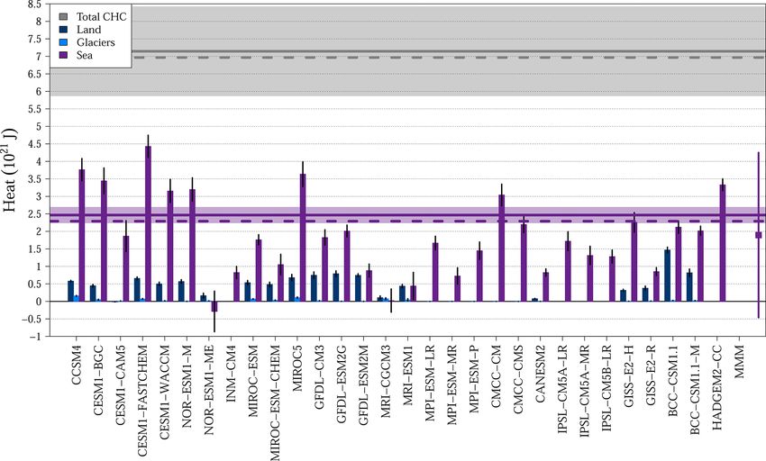
584                                                              F. J. Cuesta-Valero et al.: Earth heat inventory in CMIP5 models

Table 1. Variables from the CMIP5 archive employed to estimate the heat content within each climate subsystem by each GCM (Sect. 2).
References for each GCM Historical experiment are also provided. All variables correspond with the r1i1p1 realization of the Historical
experiment. A description of all listed variables can be found at the dedicated web page of the Lawrence Livermore National Laboratory
(LLNL, 2010).

  Model                   Ocean        Land         Atmosphere            Cryosphere               TOA                References
                                                                                                   imbalance
  CCSM4                   so, thetao   mrlsl, tsl   hus, ps, ta, ua, va   mrfso, sic, sit, snw     rlut, rsdt, rsut   Gent et al. (2011)
  CESM1-BGC               so, thetao   mrlsl, tsl   hus, ps, ta, ua, va   mrfso, sic, sit, snw     rlut, rsdt, rsut   Long et al. (2013)
  CESM1-CAM5              so, thetao   mrlsl, tsl   hus, ps, ta, ua, va   mrfso, sic, sit, snw     rlut, rsdt, rsut   Meehl et al. (2013)
  CESM1-FASTCHEM          so, thetao   mrlsl, tsl   hus, ps, ta, ua, va   mrfso, sic, sit, snw     rlut, rsdt, rsut   Hurrell et al. (2013)
  CESM1-WACCM             so, thetao   mrlsl, tsl   hus, ps, ta, ua, va   mrfso, sic, sit, snw     rlut, rsdt, rsut   Marsh et al. (2013)
  NOR-ESM1-M              so, thetao   mrlsl, tsl   hus, ps, ta, ua, va   mrfso, sic, sit, snw     rlut, rsdt, rsut   Iversen et al. (2013)
  NOR-ESM1-ME             so, thetao   mrlsl, tsl   hus, ps, ta, ua, va   mrfso, sic, sit, snw     rlut, rsdt, rsut   Tjiputra et al. (2013)
  INM-CM4                 so, thetao   mrlsl, tsl   hus, ps, ta, ua, va   sic, sit, snw            rlut, rsdt, rsut   Volodin et al. (2010)
  MIROC-ESM               so, thetao   mrlsl, tsl   hus, ps, ta, ua, va   mrfso, sic, sit, snw     rlut, rsdt, rsut   Watanabe et al. (2011)
  MIROC-ESM-CHEM          so, thetao   mrlsl, tsl   hus, ps, ta, ua, va   mrfso, sic, sit, snw     rlut, rsdt, rsut   Watanabe et al. (2011)
  MIROC5                  so, thetao   mrlsl, tsl   hus, ps, ta, ua, va   mrfso, sic, sit, snw     rlut, rsdt, rsut   Watanabe et al. (2010)
  GFDL-CM3                so, thetao   mrlsl, tsl   hus, ps, ta, ua, va   mrfso, sic, sit, snw     rlut, rsdt, rsut   Donner et al. (2011)
  GFDL-ESM2G              so, thetao   mrlsl, tsl   hus, ps, ta, ua, va   mrfso, sic, sit, snw     rlut, rsdt, rsut   Dunne et al. (2012)
  GFDL-ESM2M              so, thetao   mrlsl, tsl   hus, ps, ta, ua, va   mrfso, sic, sit, snw     rlut, rsdt, rsut   Dunne et al. (2012)
  MRI-CGCM3               so, thetao   mrso, tsl    hus, ps, ta, ua, va   mrfso, sic, sit, snw     rlut, rsdt, rsut   Yukimoto et al. (2012)
  MRI-ESM1                so, thetao   mrso, tsl    hus, ps, ta, ua, va   mrfso, sic, sit, snw     rlut, rsdt, rsut   Adachi et al. (2013)
  MPI-ESM-LR              so, thetao   mrso, tsl    hus, ps, ta, ua, va   sic, sit, snw            rlut, rsdt, rsut   Giorgetta et al. (2013)
  MPI-ESM-MR              so, thetao   mrso, tsl    hus, ps, ta, ua, va   sic, sit, snw            rlut, rsdt, rsut   Giorgetta et al. (2013)
  MPI-ESM-P               so, thetao   mrso, tsl    hus, ps, ta, ua, va   sic, sit, snw            rlut, rsdt, rsut   Jungclaus et al. (2014)
  CMCC-CM                 so, thetao   mrso, tsl    hus, ps, ta, ua, va   sic, sit, snw            rlut, rsdt, rsut   Scoccimarro et al. (2011)
  CMCC-CMS                so, thetao   mrso, tsl    hus, ps, ta, ua, va   sic, sit, snw            rlut, rsdt, rsut   Scoccimarro et al. (2011)
  CANESM2                 so, thetao   mrlsl, tsl   hus, ps, ta, ua, va   mrfso, sic, sit, snw     rlut, rsdt, rsut   Arora et al. (2011)
  IPSL-CM5A-LR            so, thetao   mrso, tsl    hus, ps, ta, ua, va   sic, sit                 rlut, rsdt, rsut   Dufresne et al. (2013)
  IPSL-CM5A-MR            so, thetao   mrso, tsl    hus, ps, ta, ua, va   sic, sit                 rlut, rsdt, rsut   Dufresne et al. (2013)
  IPSL-CM5B-LR            so, thetao   mrso, tsl    hus, ps, ta, ua, va   sic, sit                 rlut, rsdt, rsut   Dufresne et al. (2013)
  GISS-E2-H               so, thetao   mrlsl, tsl   hus, ps, ta, ua, va   mrfso, sic, sit, snw     rlut, rsdt, rsut   Miller et al. (2014)
  GISS-E2-R               so, thetao   mrlsl, tsl   hus, ps, ta, ua, va   mrfso, sic, sit, snw     rlut, rsdt, rsut   Miller et al. (2014)
  BCC-CSM1.1              so, thetao   mrlsl, tsl   hus, ps, ta, ua, va   mrfso, sic, sit, snw     rlut, rsdt, rsut   Wu et al. (2014)
  BCC-CSM1.1-M            so, thetao   mrlsl,tsl    hus, ps, ta, ua, va   mrfso, sic, sit, snw     rlut, rsdt, rsut   Wu et al. (2014)
  HADGEM2-CC              so, thetao   mrlsl, tsl   hus, ps, ta, ua, va   mrfso, sic, sit, snw     rlut, rsdt, rsut   Collins et al. (2011)

8s is the surface geopotential estimated from orography                   et al., 2013). Therefore, the cryosphere heat content was es-
(in m2 s−2 ); and Ti , ki , qi and 1pi are the air temperature            timated as
(in K), specific kinetic energy (in J kg), specific humidity
(in kg kg−1 ) and thickness (in Pa) of the ith atmospheric                QCryosphere = Lf · (1ω + ρ · 1p · 1z + 1),                         (4)
layer, respectively.
   For estimating the CHC series, the simulated cryosphere                where QCryosphere is absorbed heat per surface unit
was divided into three terms: sea ice, subsurface ice and                 (in J m−2 ), ρ = 920 kg m−3 is ice density (Rhein et al.,
glaciers. Variations in the mass of simulated sea ice and                 2013), 1ω is the change in subsurface ice mass per surface
subsurface ice were multiplied by the latent heat of fusion               unit (in kg m−2 ), 1p is the change in the proportion of sea
(Lf = 3.34×10⁵ J kg−1 ; Rhein et al., 2013) to obtain the heat            ice at each ocean grid cell, 1z is the change in thickness of
absorbed in the melting process. The same method was ap-                  sea ice at each ocean grid cell (in m), and 1 is the change
plied to the change in snow mass in grid cells containing land            in snow amount at each cell containing land ice (in kg m−2 ).
ice within each CMIP5 GCM (glaciers or ice sheets, sftgif                 It is important to note that nine of the CMIP5 GCMs did not
variable in the CMIP5 archive). Although this is not a sat-               provide outputs for the subsurface ice amount (mrfso vari-
isfactory approach given the differences between snow and                 able) and that three of the models did not provide outputs
land ice, it is the only available approximation since CMIP5              for snow amount (snw variable; see Table 1), and thus these
GCMs do not typically represent terrestrial ice masses (Flato             terms are missing in the CHC estimates from those models.
                                                                          We were unable to retrieve the file indicating the cells con-

Earth Syst. Dynam., 12, 581–600, 2021                                                            https://doi.org/10.5194/esd-12-581-2021
F. J. Cuesta-Valero et al.: Earth heat inventory in CMIP5 models 585
taining land ice (sftgif file) for the HADGEM2-CC GCM;
thus we used the CMCC-CMS sftgif file interpolated to the
HADGEM2-CC grid, since the grid for both models have
a similar spatial resolution (1.25◦ × 1.875◦ for HADGEM2-
CC; 1.875◦ × 1.875◦ for CMCC-CMS).
Estimates of total heat in the climate system from each
CMIP5 model are required to determine the simulated parti-
tion of heat among each climate subsystem. The total heat
content can be determined as the sum of the heat storage
within the different climate subsystems (Earth heat content,
EHC) or as the integration of the radiative imbalance at the
top of the atmosphere (N) during the period of interest. Both
approximations have been used in the literature and are con-
sidered equivalent (Rhein et al., 2013; Palmer and McNeall,
2014; Trenberth et al., 2014; von Schuckmann et al., 2016).
That is, if a model does not produce artificial sources or leak-
ages of energy or mass (i.e. if the model conserves the total
heat content in the system), the change in N and in EHC
Figure 1. Example to illustrate the process to estimate heat propor-
should be almost identical (Hobbs et al., 2016). Neverthe-
tions using data from the CCSM4 Historical simulation. In this case,
less, CMIP5 GCM simulations are prone to drift, particularly
the proportion of heat within the continental subsurface (GHC / N)
the ocean component due to incomplete model spin-up pro- is estimated as the slope from the linear regression analysis (solid
cedures (Sen Gupta et al., 2013; Séférian et al., 2016). For line) between the simulated GHC and N anomalies (dots) for the pe-
this reason, potential drifts in estimates of heat content and riod 1972–2005 CE multiplied by 100. The proportion of heat in the
the components of the radiative budget at the top of the at- rest of the climate subsystems is estimated by replacing the GHC
mosphere were removed by subtracting the linear trend of anomaly with the corresponding heat content anomaly. The EHC
the corresponding preindustrial control simulation from the anomaly is also used as the metric for the total heat content in the
Historical simulations, which should correct artificial drifts system by replacing the N anomaly in the regression analysis.
in the simulated heat content within each climate subsystem
(Hobbs et al., 2016). N estimates from the CESM1-CAM5
GCM constitute a particular case, since an unrealistic trend continental subsurface, AHC / N and AHC / EHC for the
remained in the Historical experiment in comparison with simulated proportion of heat in the atmosphere, and CHC / N
other CMIP5 GCMs after removing the drift using data from and CHC / EHC for the simulated proportion of heat ab-
the corresponding control simulation (Fig. S2). The rest of sorbed by the cryosphere.
the variables from this GCM were dedrifted using the trend
estimated from the preindustrial control simulation as in the
3 Results
other CMIP5 simulations, but the drift in the outgoing short-
wave radiation and the outgoing longwave radiation at the 3.1 Earth heat inventory
top of the atmosphere could not be removed. Therefore, we
used the trend estimated from the first five decades of the The CMIP5 ensemble mean overestimates the observed
Historical simulation (1861–1911 CE) to remove the drift in ocean heat content for the period 1972–2005 CE and under-
N estimates, achieving a better comparison with the other estimates the observations for the continental subsurface and
CMIP5 GCMs (Fig. S2). the cryosphere (Fig. 2). Additionally, the multimodel mean
As a complement to the estimates of the EHI detailed yields higher total heat in the climate system than observa-
above, we also estimated the partition of the simulated to- tions, as expected due to the high OHC values reached by
tal heat content among the ocean, the continental subsurface, these simulations (Fig. 2a). Indeed, the CMIP5 multimodel
the atmosphere and the cryosphere. A linear regression anal- mean yields an OHC increase of 247 ± 172 ZJ (mean ± 2 SD
ysis was performed between the evolution of the simulated (standard deviations), 1 ZJ = 1 × 10²¹ J) for 1972–2005 CE,
heat storage within each climate subsystem and the estimates higher than the observational estimates in Church et al.
of total heat content in the entire climate system to deter- (2011) (∼ 199 ZJ) and von Schuckmann et al. (2020) (164 ±
mine the partition of heat within the four climate subsystems 17 ZJ, Table 2). These high OHC estimates are the cause
(Fig. 1). The slope of the linear fit was assumed to represent of the large Earth heat content displayed by the CMIP5 en-
the simulated proportion of heat in the corresponding subsys- semble, since the EHC estimates result from the cumulative
tem, thus providing estimates of OHC / N and OHC / EHC heat storage in the four climate subsystems, and the ocean
for the simulated proportion of heat in the ocean, GHC / N accounts for around 90 % of the total heat storage (Church
and GHC / EHC for the simulated proportion of heat in the et al., 2011; Hansen et al., 2011; Rhein et al., 2013; Gleck-
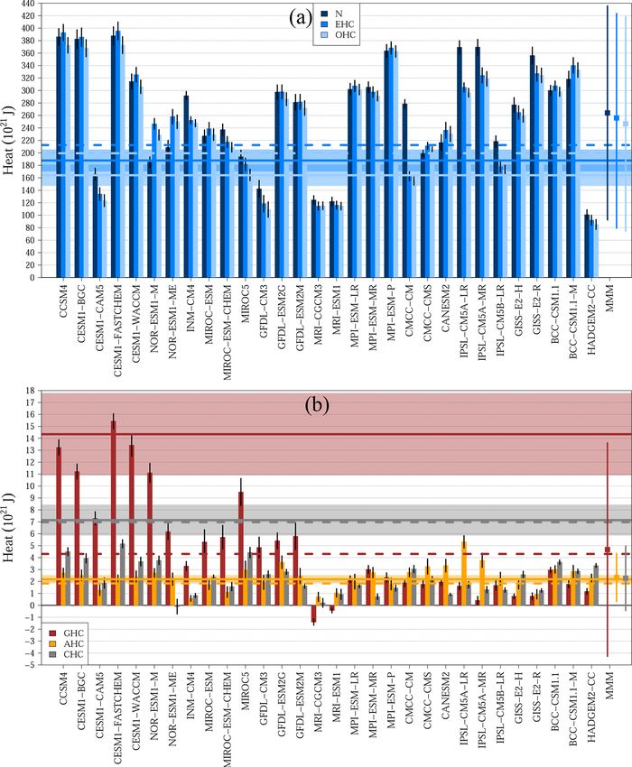
https://doi.org/10.5194/esd-12-581-2021 Earth Syst. Dynam., 12, 581–600, 2021586 F. J. Cuesta-Valero et al.: Earth heat inventory in CMIP5 models Figure 2. Simulated heat storage for 1972–2005 CE from 30 CMIP5 GCM Historical simulations. (a) Results for N (dark blue bars), EHC (blue bars) and OHC (light blue bars). (b) Results for GHC (brown bars), AHC (orange bars) and CHC (grey bars). Vertical black lines at the top of the bars indicate the 95 % confidence interval for each model. Observations from von Schuckmann et al. (2020) are shown as solid horizontal lines and shadows (mean and 95 % confidence intervals), and observations from Church et al. (2011) are displayed as dashed horizontal lines. Multimodel means and 95 % confidence intervals are indicated in the right side of the panel (MMM). ler et al., 2016; von Schuckmann et al., 2020). The integra- verge from those for the Earth heat content in some mod- tion of the radiative imbalance at the top of the atmosphere els, which may suggest that those models have biases in for the period 1972–2005 CE should yield similar values to their represented energy budget. Particularly, the CESM1- those of EHC and OHC over the same period, as the ra- CAM5, CMCC-CM, GFDL-CM3, HADGEM2-CC, INM- diative imbalance causes the heat storage within the differ- CM4, IPSL-CM5A-LR, IPSL-CM5A-MR, IPSL-CM5B-LR, ent climate subsystems. Indeed, EHC and OHC estimates NOR-ESM1-M and NOR-ESM1-ME models show N-EHC are generally similar within each model, while N values di- differences larger than 10 % of their simulated changes in Earth Syst. Dynam., 12, 581–600, 2021 https://doi.org/10.5194/esd-12-581-2021
F. J. Cuesta-Valero et al.: Earth heat inventory in CMIP5 models                                                             587

Table 2. Earth heat inventory and proportion of heat allocated      of GHC in the CMIP5 GCMs is markedly limited by the sim-
in each climate subsystem from the 30 CMIP5 GCMs analysed           ulated subsurface volume, which is determined by the depth
here (MMM), and observations from Church et al. (2011) (Ch11)       of the land surface model (LSM) component (Stevens et al.,
and von Schuckmann et al. (2020) (vS20). Heat storage in ZJ, heat   2007; MacDougall et al., 2008; Cuesta-Valero et al., 2016).
proportion in %.                                                    Indeed, five of seven GCMs using LSM components deeper
                                                                    than 40 m yield GHC estimates are in agreement with the
  Magnitude                        MMM      Ch11         vS20       95 % confidence interval of observations from von Schuck-
  N                            264 ± 171        –            –      mann et al. (2020), suggesting that the underestimated conti-
  EHC                          256 ± 177      212    188 ± 17       nental heat storage and the large spread in the CMIP5 ensem-
  OHC                          247 ± 172      199    164 ± 17       ble are direct consequences of the different bottom boundary
  GHC                              5±9          4       14 ± 3      depths used by each model (see Cuesta-Valero et al., 2016,
  AHC                              2±2          2    2.2 ± 0.3      for a complete list of bottom boundary depths). The nega-
  CHC                              2±3          7        7±1        tive GHC estimates for both MRI simulations in Fig. 2b are
  CHC (only sea ice)               2±2          2    2.5 ± 0.2
                                                                    caused by an unrealistic and sharp decrease in the total water
  OHC / N                        93 ± 24         –           –      content in the subsurface along these Historical simulations
  OHC / EHC                        96 ± 4      94     88 ± 12       (see Cuesta-Valero et al., 2016, for more details).
  OHC / EHC (only sea ice)         96 ± 4      96     90 ± 12          The CMIP5 ensemble mean constantly underestimates
  GHC / N                           2±3          –           –      the cryosphere heat content in comparison with observa-
  GHC / EHC                         2±3          2       7±2        tions (Fig. 2b). The multimodel average estimates a 2 ± 3 ZJ
  GHC / EHC (only sea ice)          2±3          2       7±2
                                                                    change in the cryosphere heat content for the period 1972–
  AHC / N                       1.0 ± 0.9        –           –
  AHC / EHC                         1±1        0.9   1.1 ± 0.2
                                                                    2005 CE, which is much lower than the observed CHC in
  AHC / EHC (only sea ice)          1±1        0.9   1.1 ± 0.2      Church et al. (2011) (7 ZJ) and in von Schuckmann et al.
  CHC / N                           1±1          –           –      (2020) (7 ± 1 ZJ, Table 2). Figure 3 examines the three com-
  CHC / EHC                         1±1          3   3.6 ± 0.7      ponents contributing to the cryosphere heat content in this
  CHC / EHC (only sea ice)          1±1          1   1.2 ± 0.2      analysis for each CMIP5 model (i.e. sea ice, subsurface ice
                                                                    and glaciers), in order to understand the reason for the dis-
                                                                    agreement between simulated and observed CHC estimates.
                                                                    The simulated heat uptake to reduce sea ice volume is in
OHC (Fig. 2a). Furthermore, the inter-model spread obtained         agreement with observations, with a multimodel mean of
for these three magnitudes is excessively large, given that all     2 ± 2 ZJ, while observations reach ∼ 2 and 2.5 ± 0.2 ZJ in
Historical simulations were forced using the same boundary          Church et al. (2011) and von Schuckmann et al. (2020),
conditions – i.e. the same external forcing. Further details        respectively (Fig. 3, Table 2). However, the spread in the
about the large spread among the CMIP5 simulations as well          CMIP5 results is still large, with the difference between the
as the discrepancies in N, EHC and OHC can be found in the          highest and the lowest estimates of heat storage due to sea
Discussion section.                                                 ice melting being more than double the value of the ensem-
   A different situation is found for the magnitude of the sim-     ble mean (5 ZJ). Heat uptake by subsurface ice is the second
ulated heat storage within the continental subsurface, with         contributor to the cryosphere heat content in all models after
the CMIP5 ensemble mean yielding generally lower esti-              sea ice melting. Nevertheless, neither Church et al. (2011)
mates of GHC than the observations (Fig. 2b). The multi-            nor von Schuckmann et al. (2020) include observations of the
model mean achieves a GHC change of 5 ± 9 ZJ for 1972–              change in terrestrial subsurface ice, and not all CMIP5 GCMs
2005 CE, which is lower than the 14 ± 3 ZJ in von Schuck-           include a representation of the subsurface ice masses; thus
mann et al. (2020) but similar to the ∼ 4 ZJ in Church et al.       we cannot assess the ability of the CMIP5 GCMs to repro-
(2011) (Table 2). However, the difference between the GHC           duce this term of the cryosphere heat content. Furthermore,
estimates in Church et al. (2011) and in von Schuckmann             the approximation used in this study to estimate the simu-
et al. (2020) is large (Fig. 2), probably caused by the differ-     lated heat absorbed by glaciers yields a much smaller value
ent source of data used in both products. That is, results from     from models than from observations (∼ 2.8 ZJ in Church
Church et al. (2011) are based on surface air temperatures          et al., 2011 and ∼ 1.4 ZJ in von Schuckmann et al., 2020),
while results from von Schuckmann et al. (2020) are based           indicating that a comprehensive representation of terrestrial
on subsurface temperatures (see Huang, 2006; Cuesta-Valero          ice masses is necessary to reproduce observations.
et al., 2021, and the Data and methods section for more de-            The heat storage within the atmosphere yields the best
tails). Therefore, the estimate of 14 ± 3 ZJ from von Schuck-       results for the CMIP5 GCMs in comparison with observa-
mann et al. (2020) constitutes a more robust reference for          tions (Fig. 2b). The CMIP5 ensemble mean achieves an at-
evaluating the simulated ground heat content by the CMIP5           mosphere heat content of 2 ± 2 ZJ, in agreement with obser-
ensemble, indicating that models underestimate observations         vations from Church et al. (2011) (2 ZJ) and von Schuck-
of continental heat storage. Additionally, the representation       mann et al. (2020) (2.2 ± 0.3 ZJ). Additionally, one-third of

https://doi.org/10.5194/esd-12-581-2021                                                Earth Syst. Dynam., 12, 581–600, 2021
588 F. J. Cuesta-Valero et al.: Earth heat inventory in CMIP5 models
Figure 3. Simulated CHC for 1972–2005 CE. Dark blue bars indicate the heat uptake due to changes in subsurface ice mass, blue bars
indicate the heat uptake due to changes in glacier mass, and purple bars indicate the heat uptake due to changes in sea ice volume (see Sect. 2
for details). Vertical black lines at the top of the bars indicate the 95 % confidence interval for each model. The multimodel mean and 95 %
confidence interval for the heat uptake due to changes in sea ice volume are indicated in the right side of the panel (MMM). Observations
from von Schuckmann et al. (2020) are shown as solid horizontal lines and shadows (means and 95 % confidence intervals), and observations
from Church et al. (2011) are displayed as dashed horizontal lines.
the models displays AHC estimates within the 95 % confi- and 5, Table 2). Nevertheless, the ensemble mean presents
dence interval of the observed atmosphere heat content. De- a partition of heat in each climate subsystem similar to the
spite the similarity between the multimodel mean and obser- results for the EHI. That is, the simulated proportion of en-
vations, the inter-model spread is large, with the difference ergy in the ocean is larger than observations, the proportion
between the maximum and minimum AHC from CMIP5 of heat in the continental subsurface and in the cryosphere
models reaching 5 ZJ, more than double the value of the ob- is lower than observations, and the proportion of heat in the
servational estimate. atmosphere is in agreement with observations. Additionally,
results vary depending on the metric used to characterize to-
tal heat content in the system, particularly for the ocean.
3.2 Heat partition within climate subsystems All 30 CMIP5 GCM simulations represent a proportion of
heat stored in the ocean within the 95 % confidence interval
The simulated heat storage within each climate subsystem of the observations considering EHC as the metric for to-
has been assessed in the previous section, displaying a large tal energy in the climate system (OHC / EHC, blue dots in
inter-model spread among CMIP5 GCMs. This wide range Fig. 4a), achieving a multimodel mean just 2 % higher than
of results hampers the assessment of the simulated Earth Church et al. (2011) and 8 % higher than von Schuckmann
heat inventory, particularly the evaluation of the represented et al. (2020) (Table 2). The spread of OHC / EHC estimates is
ocean heat content and total heat in the climate system. Nev- small, with values ranging from 91±2 % (MIROC5) to 100±
ertheless, models may be distributing the total heat content 1 % (MRI-CGCM3). Nevertheless, the simulated proportion
among the four climate subsystems similarly. This section of heat in the ocean presents different results for some mod-
evaluates the partition of heat among climate subsystems els when considering the integration of the radiative imbal-
within each CMIP5 GCM, testing whether models simulat- ance at the top of the atmosphere as the metric for total heat
ing higher values of N and EHC distribute this energy in the in the climate system (OHC / N, black dots in Fig. 4a). The
same proportion among climate subsystems as models simu- model spread is much larger for OHC / N estimates than for
lating lower values of total heat content. OHC / EHC estimates, ranging from 56 ± 2 % (CMCC-CM)
The simulated heat partitions by the 30 CMIP5 GCMs to 122 ± 4 % (NOR-ESM1-M). These different estimates are
achieve a lower inter-model spread in comparison with the related to the differences between N and EHC values dis-
simulated EHI, particularly for the ocean component (Figs. 4
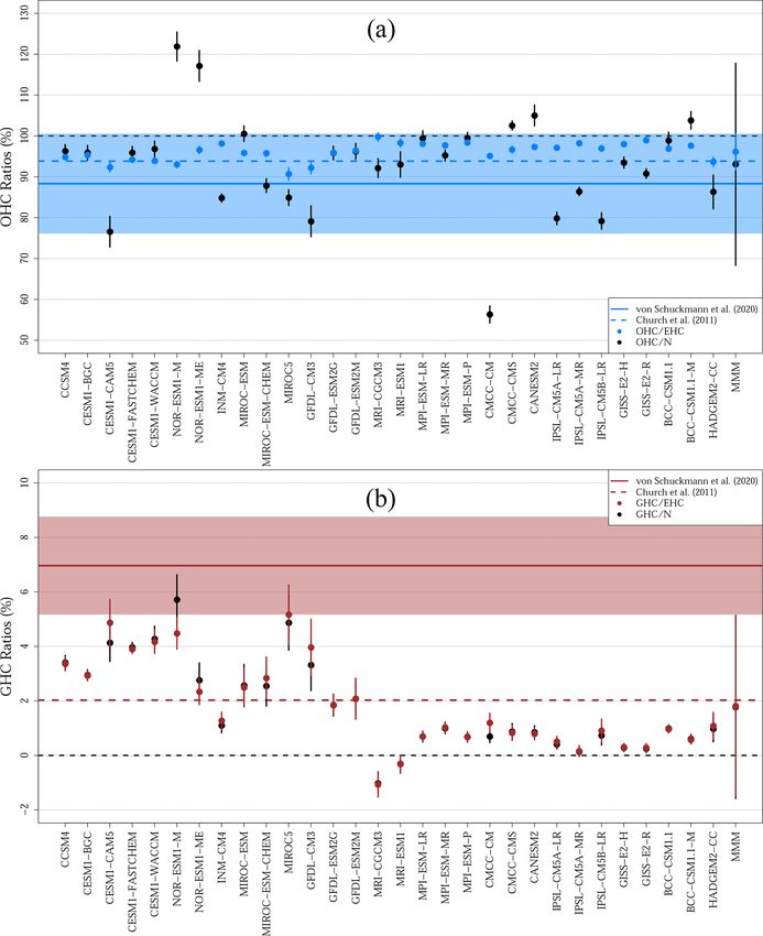
Earth Syst. Dynam., 12, 581–600, 2021 https://doi.org/10.5194/esd-12-581-2021F. J. Cuesta-Valero et al.: Earth heat inventory in CMIP5 models 589 Figure 4. (a) Simulated proportion of heat within the ocean for the period 1972–2005 CE using EHC (blue dots) and N (black dots) as estimates of total heat content in the climate system. (b) Simulated proportion of heat within the continental subsurface for the period 1972– 2005 CE using EHC (red dots) and N (black dots) as estimates of total heat content in the climate system. Observations from von Schuckmann et al. (2020) are shown as solid horizontal lines and shadows (means and 95 % confidence intervals), and observations from Church et al. (2011) are displayed as dashed horizontal lines. Multimodel means and 95 % confidence intervals are indicated in the right side of the panels (MMM). Black dashed lines indicate the 0 % and 100 % values. played in Fig. 2a. That is, some CMIP5 models yield exces- in those models is much lower than EHC estimates (the sively different values of N and EHC, suggesting the pres- BCC-CSM1.1-M, CANESM2, CMCC-CMS, MIROC-ESM, ence of non-conservation terms in the simulated energy bud- NOR-ESM-M and NOR-ESM-ME models in Fig. 4a). The get (see Sects. 3.1 and 4). Six models obtain OHC / N es- opposite behaviour occurs in other five models that simulate timates above 100 %, which indicates that the simulated N OHC / N values below 80 % (the CESM1-CAM5, CMCC- https://doi.org/10.5194/esd-12-581-2021 Earth Syst. Dynam., 12, 581–600, 2021
590                                                               F. J. Cuesta-Valero et al.: Earth heat inventory in CMIP5 models

Figure 5. (a) Simulated proportion of heat within the atmosphere for the period 1972–2005 CE using EHC (orange dots) and N (black dots) as
estimates of total heat content in the climate system. (b) Simulated proportion of heat within the continental subsurface for the period 1972–
2005 CE using EHC (light blue dots) and N (black dots) as estimates of total heat content within the climate system. Observations from
von Schuckmann et al. (2020) are shown as solid horizontal lines and shadows (means and 95 % confidence intervals), and observations from
Church et al. (2011) are displayed as dashed horizontal lines. Multimodel means and 95 % confidence intervals are indicated in the right side
of the panels (MMM). The black dashed line indicate the 0 % value.

CM, GFDL-CM3, IPSL-CM5A-LR and IPSL-CM5B-LR                              et al., 2014; Hobbs et al., 2016; von Schuckmann et al.,
models in Fig. 4a), which is probably an excessively small               2016, 2020).
proportion of heat stored in the ocean in comparison with                   Estimates of the proportion of heat in the ground from
observations (Hansen et al., 2011; Palmer et al., 2011;                  CMIP5 GCMs show smaller differences between GHC / N
Rhein et al., 2013; Palmer and McNeall, 2014; Trenberth                  and GHC / EHC than the retrieved proportion of heat in the

Earth Syst. Dynam., 12, 581–600, 2021                                                         https://doi.org/10.5194/esd-12-581-2021
F. J. Cuesta-Valero et al.: Earth heat inventory in CMIP5 models                                                                 591

ocean (Fig. 4b). Both GHC / N and GHC / EHC estimates
have a multimodel mean and 95% confidence interval of
2 ± 3 %, which is in agreement with estimates derived from
Church et al. (2011) (∼ 2 %), but excessively low in compari-
son with results from von Schuckmann et al. (2020) (7±2 %).
As in the case of the simulated ground heat content, the rel-
atively large inter-model spread in the simulated proportion
of heat stored in the continental subsurface is caused by the
depth of the LSM component. Indeed, deeper models reach
higher proportions of heat in the ground than shallower mod-
els using either EHC or N as the metric for total heat in the
climate system. This marked dependence on the depth of the       Figure 6. Correlation coefficients between the simulated equi-
represented subsurface is apparent in a covariance analysis,     librium climate sensitivity (ECS, squares), transient climate re-
                                                                 sponse (TCR, circles), adjusted forcing (AF, triangles), depth of
with significant correlation coefficients between the depth of
                                                                 the LSM component (LSM depth, diamonds) and the components
the LSM component and the GHC / N and GHC / EHC esti-
                                                                 of the Earth heat inventory. Results obtained by analysing the 18
mates (Fig. S3).                                                 models presenting estimates of ECS, TCR and AF in Forster et al.
   As in the case of the continental subsurface, CMIP5           (2013). Red symbols indicate statistically significant results at the
GCMs consistently underestimate the observed proportion          95 % confidence level using a Student’s t test. The dashed black
of heat absorbed by the cryosphere. Both metrics of total        horizontal line indicates zero values.
heat content in the system yield similar ratios (CHC / N
and CHC / EHC), with only one model (the HADGEM2-
CC) reaching the 95 % confidence interval from von Schuck-       rium climate sensitivities in the literature (e.g. Knutti et al.,
mann et al. (2020) (Fig. 5). This disagreement between ob-       2017). Indeed, Forster et al. (2013) assessed the response to
servations and CMIP5 simulations is expected given the           the common forcing of a large ensemble of CMIP5 GCMs
large differences in the simulated and observed cryosphere       in terms of climate sensitivity, feedbacks and adjusted radia-
heat content (Fig. 2b), while the partial agreement between      tive forcing, showing that these models yielded a broad range
the HADGEM2-CC estimates and the observations is likely          of responses. To test the potential relationship between to-
the result of the low EHC and N values simulated by this         tal heat storage and model response, we performed a covari-
model (Fig. 2a). Nevertheless, CMIP5 models and observa-         ance analysis between some of the metrics used by Forster
tions agree if considering only the heat allocated for sea ice   et al. (2013) to characterize the response of CMIP5 models
melting (Table 2), with the multimodel average yielding an       and the estimated Earth heat inventory here (Fig. 6). The 18
average of 1±1 % in comparison with 1 % from Church et al.       CMIP5 models in common with those analysed in Forster
(2011) and 1.2 ± 0.2 % from von Schuckmann et al. (2020).        et al. (2013) do not show covariance between the heat stor-
   The CMIP5 GCMs also show similar estimates for the pro-       age within the different climate subsystems and equilibrium
portion of heat in the atmosphere using both EHC and N met-      climate sensitivity nor with the transient climate response.
rics. A large proportion of the models achieve AHC / N and       However, the adjusted forcing during the last part of the His-
AHC / EHC ratios within the 95 % confidence interval from        torical experiment (2001–2005 CE) presents significant cor-
von Schuckmann et al. (2020) and contain the observational       relation coefficients with N, EHC and OHC (red triangles in
estimates from Church et al. (2011) within the limits of their   Fig. 6). This is a reasonable result, as different adjusted forc-
individual confidence intervals (Fig. 5). The ensemble aver-     ings result from a spread of radiative imbalances at the top of
age yields a proportion of heat in the atmosphere of around      the atmosphere and climate sensitivities, from which differ-
1 ± 1 %, with observations reporting 0.9 % (Church et al.,       ent N values arise – and therefore distinct heat storage within
2011) and 1.1 ± 0.2 %, which is a reassuring result for the      the ocean (Palmer and McNeall, 2014). The relationship be-
CMIP5 models (von Schuckmann et al., 2020, Table 2).             tween adjusted forcing and heat storage, nevertheless, should
                                                                 be considered just as a potential line of research, since the
                                                                 estimates of radiative forcing from transient climate simula-
4   Discussion                                                   tions depend on the method employed in the analysis (Forster
                                                                 et al., 2016), meaning that further work is needed to evaluate
The 30 CMIP5 GCMs analysed here simulate markedly dif-           the robustness of this relationship.
ferent total heat contents within the climate system, indepen-      The simulated proportion of heat in the ocean for some
dently of the analysed metric (N, EHC and OHC values in          models shows markedly different results depending on the
Fig. 2a), which may be caused by the different response from     metric used for total heat content in the climate system
each model to the common Historical forcing. That is, differ-    (Fig. 4a). The different heat partition is caused by the dis-
ent models simulate distinct responses to the common exter-      crepancies between estimates of N and EHC within each
nal forcing, as seen in the broad range of simulated equilib-    GCM simulation (Fig. 2a), which are probably related to

https://doi.org/10.5194/esd-12-581-2021                                               Earth Syst. Dynam., 12, 581–600, 2021
592 F. J. Cuesta-Valero et al.: Earth heat inventory in CMIP5 models non-conservation terms in the simulated energy budget by ers snow changes in grid cells indicated as land ice by the each GCM as discussed in Hobbs et al. (2016). That is, small models, but results show that this method markedly underes- numerical inconsistencies, insufficient spin-up time, or the timates heat uptake in comparison with observations (Fig. 3). amount of water leaving the LSM component at the bottom Furthermore, the observed proportion of heat in the ocean of the soil column, among other factors, may prevent the con- yields different results if considering the whole cryosphere servation of energy in GCM simulations (Sen Gupta et al., for estimating EHC or if considering only the change in sea 2013; Hobbs et al., 2016; Séférian et al., 2016; Trenberth ice volume (Table 2). Therefore, heat uptake by terrestrial et al., 2016). We applied a simple drift-removal technique ice sheets and glaciers is important to improve the simulated to each variable considered in this study in order to minimize EHI and the partition of heat within the four climate subsys- the effect of possible non-conservation terms in our results tems. CMIP5 GCMs currently include modules representing (see Sect. 2). This method has shown good results in previ- ice sheets, but such model components were not activated ous analyses including several CMIP5 experiments, although for generating the CMIP5 simulations analysed here, prob- no perfect solution is available yet (Hobbs et al., 2016). ably due to issues with computational resources and techni- The low ground heat content achieved by the shallow cal challenges of coupling the ice sheet grids with the rest LSM components (Fig. 2b) alters the distribution of heat of the subsystems (Flato et al., 2013). New experiments are within models, mainly causing a higher proportion of heat planned to assess the ability of the latest generation of GCMs stored in the ocean if considering EHC as the metric for to- to reproduce the ice sheets of Greenland and Antarctica tal heat content. This can be seen in a covariance analysis within the sixth phase of the Coupled Model Intercompari- between OHC / EHC estimates and the depth of the LSM son Project (CMIP6), including coupled atmosphere–ocean– components in the CMIP5 ensemble (Fig. S3). The shal- ice-sheet simulations (Nowicki et al., 2016). Although these low depth of the LSM components included in the CMIP5 experiments are focused on understanding the contribution GCMs limits the represented amount of continental heat stor- of ice sheets to sea-level rise, these simulations could be also age within each simulation (Stevens et al., 2007; MacDougall useful to test whether including land ice masses enhances the et al., 2008; Cuesta-Valero et al., 2016; Hermoso de Mendoza representation of the Earth heat inventory within GCMs, par- et al., 2020), altering the GHC estimates and the obtained ticularly the coupled experiments. GHC / EHC and GHC / N ratios from the 30 CMIP5 GCMs analysed here (Figs. 2b, 4b and S3). Simulated OHC / N val- ues, nevertheless, do not present such covariance with the 5 Conclusions depth of the LSM component, nor the simulated propor- tion of heat in the atmosphere and the cryosphere (Figs. S3 The ensemble of CMIP5 GCMs analysed here overestimates and S4). Surprisingly, the simulated CHC indicates signifi- the amount of heat stored in the ocean and underestimates cant covariance with the depth of the employed LSM com- the heat uptake by the cryosphere and the continental subsur- ponent (red diamond in Fig. 6), although this should be the face, while representing changes in atmosphere heat storage result of the different subsurface volume within CMIP5 mod- similar to observations. Models present a large inter-model els. That is, deeper models tend to simulate more subsurface spread of ocean heat content and total heat content in the ice and GHC than shallower models, and therefore more heat system, probably related to the wide range of simulated re- can be used to thaw the larger mass of subsurface ice. This sponses to external forcing in these GCMs. The lack of an ad- result suggests another limit to the representation of the EHI equate representation of terrestrial ice masses and continental within GCM simulations, as the lack of a sufficient continen- subsurface volume within CMIP5 models limits the amount tal subsurface volume alters the simulated heat uptake by the of heat allocated within the cryosphere and the continental subsurface ice masses. Nevertheless, further work is required subsurface. The issue of heat conservation within complex to clarify this point. numerical simulations also affects the Earth heat inventory The simulated cryosphere heat content and heat proportion represented in the CMIP5 ensemble. Nevertheless, there is are in better agreement with observations when ignoring the good agreement between simulated and observed atmosphere heat absorbed by terrestrial ice masses from the assessment, heat storage and heat uptake by changes in sea ice volume. that is, considering sea ice as the only cryosphere compo- There are two main issues hindering the assessment of the nent (see results labelled as “only sea ice” in Table 2). The EHI in CMIP5 models in comparison with observations: the same can be said about the simulated proportion of heat in the non-conservation of energy in models and the markedly dif- ocean, which shows a reduction of 2 % in the difference with ferent amounts of simulated total heat content in the Earth observations if considering only sea ice as cryosphere (Ta- system. Ocean heat storage is markedly high within the ble 2). This is caused by the lack of a representation of land CMIP5 ensemble, presenting high inter-model variability. ice in CMIP5 simulations, as only the simulated heat uptake This causes a much higher Earth heat content in the models by sea ice can be directly compared with observations, and in comparison with observations. The different response of the method used here to approximate the melting of land ice each model to the external forcing may be the cause for this in the models is not accurate enough. Our approach consid- large variability and high values of OHC and EHC, suggest- Earth Syst. Dynam., 12, 581–600, 2021 https://doi.org/10.5194/esd-12-581-2021
F. J. Cuesta-Valero et al.: Earth heat inventory in CMIP5 models                                                                 593

ing that simulations from the CMIP6 models may present an           for improvement in climate modelling for a long time now.
even larger spread in results, since Meehl et al. (2020) found      The analysis of CMIP6 simulations will allow for testing of
a larger inter-model variability for estimates of equilibrium       the improvement of advanced climate models in reproducing
climate sensitivity (ECS) in this new generation of models.         the evolution of climate change, but in order to maintain the
Otherwise, the spread in effective radiative forcing (ERF)          progress in modelling and to enhance the understanding of
is similar in CMIP5 and CMIP6 (Smith et al., 2020), and             the processes conforming the Grand Challenges of the World
the simulated radiative imbalance seems to present smaller          Climate Research Program (WCRP), the global network of
inter-model variability in the CMIP6 ensemble than in the           observations must be maintained and expanded.
CMIP5 ensemble (Wild, 2020). Therefore, a future assess-
ment of the simulated EHI within the CMIP6 ensemble is
required to determine the performance of the new genera-            Data availability. CMIP5 simulations can be accessed at the
tion of models. Regarding the non-conservation of energy            dedicated website of the Earth System Grid Federation (https:
within the models, Irving et al. (2020) have found that drifts      //esgf-node.llnl.gov/projects/cmip5/, last access: 3 May 2021)
in N and OHC are still markedly large in CMIP6 models, al-          (WCRP, 2021). Data from von Schuckmann et al. (2020) are avail-
                                                                    able at https://doi.org/10.26050/WDCC/GCOS_EHI_EXP_v2 (last
though the energy leakage within these models has improved
                                                                    access: 3 May 2021), and data from Church et al. (2011) can be
in comparison with CMIP5 simulations. Nevertheless, such
                                                                    retrieved from the publication itself.
a result indicates that an assessment of the EHI represented
by CMIP6 models will encounter similar burdens and limi-
tations to those in our analysis, including the need to apply a     Supplement. The supplement related to this article is available
drift correction technique before evaluating the simulations.       online at: https://doi.org/10.5194/esd-12-581-2021-supplement.
   The assessment of transient climate simulations in com-
parison with observations presented here indicates that
deeper continental subsurfaces and some representation of           Author contributions. FJCV designed the study, analysed the
terrestrial ice masses within GCMs are required to im-              CMIP5 simulations, and produced all results and figures. All au-
prove the simulated Earth heat inventory, as well as the as-        thors contributed to the interpretation and discussion of results.
sociated phenomena relevant to society such as sea level            FJCV wrote the paper with continuous feedback from all authors.
rise or permafrost evolution. These issues will probably be
present within the CMIP6 simulations, together with non-
conservation of energy and drifts, but the comparison with          Competing interests. The authors declare that they have no con-
observational references may help to mitigate these limita-         flict of interest.
tions in future generations of GCMs. For example, an ex-
tended sampling of the deepest part of the ocean will improve
the observational estimate of OHC and will provide a refer-         Acknowledgements. We acknowledge the World Climate Re-
                                                                    search Programme’s Working Group on Coupled Modelling, which
ence to evaluate deep heat uptake in GCMs, probably reduc-
                                                                    is responsible for CMIP, and we thank the climate modelling groups
ing the drift in these models (Irving et al., 2020; von Schuck-     responsible for the model simulations used herein (listed in Ta-
mann et al., 2020). Local and regional measurements of the          ble 1 of this paper) for producing and making available their
state of glaciers and ice sheets may help to parameterize the       model output. For CMIP the US Department of Energy’s Pro-
evolution of ice masses in individual grid cells. That is, a sim-   gram for Climate Model Diagnosis and Intercomparison provides
plified parameterization of land ice masses based on tiling         coordinating support and led development of software infrastruc-
(Essery et al., 2003; Best et al., 2004) could be implemented.      ture in partnership with the Global Organization for Earth Sys-
This strategy has been successful in representing vegetation        tem Science Portals. This analysis contributes to the PALEOLINK
functional types at sub-grid scales (Melton and Arora, 2014),       project (http://www.pastglobalchanges.org/science/wg/2k-network/
and it has been proposed to improve the representation of           projects/paleolink/intro, last access: 4 May 2021), part of the
permafrost in land surface model components (Beer, 2016).           PAGES 2k Network. Part of the presented analysis was performed
                                                                    in the computational facilities provided by the Atlantic Computa-
Additionally, expanding the global network of subsurface
                                                                    tional Excellence Network (ACENET-Compute Canada). We thank
temperature profiles will improve the estimates of continen-        two anonymous reviewers for their constructive feedback. We are
tal heat storage, mitigating the scarcity of measurements af-       grateful to Fiammetta Straneo and Susheel Adusumilli for their
ter 2000 CE and in the Southern Hemisphere (Cuesta-Valero           help with obtaining and Page 2 of 3 interpreting the sea ice vol-
et al., 2021).                                                      ume data. This work was supported by grants from the Natural
   Furthermore, the collaboration between the observational         Sciences and Engineering Research Council of Canada Discov-
and modelling communities should be maintained and ex-              ery Grant (NSERC DG 140576948), the Canada Research Chairs
panded to further advance our knowledge of key climate pro-         Program (CRC 230687), and the Canada Foundation for Innova-
cesses. Assessments of transient climate simulations based          tion (CFI) to Hugo Beltrami. Almudena García-García and Fran-
on observational estimates of important climate variables,          cisco José Cuesta-Valero are funded by Hugo Beltrami’s Canada
like the analysis performed here, have been showing paths           Research Chair program, the School of Graduate Students at

https://doi.org/10.5194/esd-12-581-2021                                                  Earth Syst. Dynam., 12, 581–600, 2021
You can also read