Comparison of ocean vertical mixing schemes in the Max Planck Institute Earth System Model (MPI-ESM1.2)
←
→
Page content transcription
If your browser does not render page correctly, please read the page content below
Geosci. Model Dev., 14, 2317–2349, 2021
https://doi.org/10.5194/gmd-14-2317-2021
© Author(s) 2021. This work is distributed under
the Creative Commons Attribution 4.0 License.

Comparison of ocean vertical mixing schemes in the Max Planck
Institute Earth System Model (MPI-ESM1.2)
Oliver Gutjahr1,a , Nils Brüggemann2,1 , Helmuth Haak1 , Johann H. Jungclaus1 , Dian A. Putrasahan1 ,
Katja Lohmann1 , and Jin-Song von Storch1,3
1 Max  Planck Institute for Meteorology, Hamburg, Germany
2 Institutfür Meereskunde, Universtät Hamburg, Hamburg, Germany
3 Center for Earth System Research and Sustainability (CEN), University of Hamburg, Hamburg, Germany
a currently at: Institut für Meereskunde, Universität Hamburg, Hamburg, Germany

Correspondence: Oliver Gutjahr (oliver.gutjahr@uni-hamburg.de)

Received: 19 June 2020 – Discussion started: 25 August 2020
Revised: 11 March 2021 – Accepted: 12 March 2021 – Published: 3 May 2021

Abstract. For the first time, we compare the effects of four   Nordic Seas lead to increased deep convection and thus to
different ocean vertical mixing schemes on the mean state      the increased overflows. Due to the warmer SSTs, the ex-
of the ocean and atmosphere in the Max Planck Institute        tratropics of the Northern Hemisphere become warmer with
Earth System Model (MPI-ESM1.2). These four schemes            TKE(+IDEMIX), weakening the meridional gradient and
are namely the default Pacanowski and Philander (1981)         thus the jet stream. With KPP, the tropics and the South-
(PP) scheme, the K-profile parameterization (KPP) from         ern Hemisphere also become warmer without weakening the
the Community Vertical Mixing (CVMix) library, a re-           jet stream. Using an energetically more consistent scheme
cently implemented scheme based on turbulent kinetic en-       (TKE+IDEMIX) produces a more heterogeneous and realis-
ergy (TKE), and a recently developed prognostic scheme         tic pattern of vertical eddy diffusivity, with lower diffusivities
for internal wave dissipation, energy, and mixing (IDEMIX)     in deep and flat-bottom basins and elevated turbulence over
to replace the often assumed constant background diffusiv-     rough topography. IDEMIX improves in particular the diffu-
ity in the ocean interior. In this study, the IDEMIX scheme    sivity in the Arctic Ocean and reduces the warm bias in the
is combined with the TKE scheme (collectively called the       Atlantic Water layer. We conclude that although shortcom-
TKE+IDEMIX scheme) to provide an energetically more            ings due to model resolution determine the global-scale bias
consistent framework for mixing, as it does not rely on the    pattern, the choice of the vertical mixing scheme may play
unwanted effect of creating spurious energy for mixing. En-    an important role for regional biases.
ergetic consistency can have implications on the climate.
Therefore, we focus on the effects of TKE+IDEMIX on the
climate mean state and compare them with the first three
schemes that are commonly used in other models but are not     1   Introduction
energetically consistent.
   We find warmer sea surface temperatures (SSTs) in           Vertical mixing in the ocean is a complex phenomenon and
the North Atlantic and Nordic Seas using KPP or                its magnitude depends on processes acting over a large range
TKE(+IDEMIX), which is related to 10 % higher over-            of vertical and horizontal scales, from about 1 km to several
flows that cause a stronger and deeper upper cell of the       metres down to centimetres (Fox-Kemper et al., 2019). Ver-
Atlantic meridional overturning circulation (AMOC) and         tical mixing affects key elements in the ocean that are of cli-
thereby an enhanced northward heat transport and higher        matic importance, such as ocean stratification, the distribu-
inflow of warm and saline water from the Indian Ocean          tion of temperature, salinity and passive tracers, the ocean
into the South Atlantic. Saltier subpolar North Atlantic and   uptake of heat and carbon, and the global meridional over-
                                                               turning circulation (MOC; e.g. Gent, 2018).

Published by Copernicus Publications on behalf of the European Geosciences Union.
2318                                      O. Gutjahr et al.: Comparison of ocean vertical mixing schemes in MPI-ESM1.2

   In ocean models, the processes that lead to mixing are          energetically more consistent scheme for vertical mixing in
subgrid scale and therefore not resolved, so they have to          the ocean. The practical effect of IDEMIX on the climate
be parameterized. The complexity of these parameteriza-            state, however, has hardly been studied, with the exception
tions varies in dependence of our understanding, application,      of the work of Nielsen et al. (2018).
and available resources (e.g. Large et al., 1994; Fox-Kemper          The four schemes, whose effect on the climate state we
et al., 2019). In fact, the parameterization of vertical mixing    investigate, are the default PP scheme from MPI-ESM1.2,
constitutes one of the current shortcomings of ocean models        KPP, TKE, and TKE+IDEMIX (see Sect. 2.1 and Ap-
(Robertson and Dong, 2019; Fox-Kemper et al., 2019).               pendix A for details). Note that we do not break down the
   Frequently used ocean vertical mixing schemes date back         effects found to the process level for which idealized un-
to the 1980s and 1990s. Often, a modelling centre or a group       coupled ocean simulations would be necessary. We have in-
decides to implement only one of these schemes and, for            corporated the Community Vertical Mixing (CVMix) library
practical reasons such as tuning effort, not to deviate from       (Griffies et al., 2015; Van Roekel et al., 2018) into MPI-
it afterwards. However, as these schemes are based on dif-         ESM1.2. The KPP scheme is already part of CVMix, and
ferent principles, deviations in the results are to be expected.   we used the infrastructure of CVMix to extend the library to
We further note that even the same scheme may produce dif-         include TKE and IDEMIX, which are not yet an official part
ferent results due to the numerical implementation (e.g. Li        of CVMix.
et al., 2019) and small modifications (e.g. Danabasoglu et al.,       The remainder of the paper is organized as follows. We
2006).                                                             first give a brief overview of the model configuration in
   In the ocean surface boundary layer, schemes diagnose           Sect. 2, with more details about the vertical mixing schemes
vertical profiles of scalar mixing diffusivity and viscosity       and the experiments we conducted. In Sect. 3, we present
from surface forcing and background fields, such as in the         the results of the comparison for the global ocean and in
Pacanowski and Philander (1981) (PP) scheme or in the K-           Sect. 4 for the regional ocean. Section 5 presents effects of
profile parameterization (KPP; Large et al., 1994). Second-        the mixing scheme in the atmosphere. Finally, we conclude
order schemes (Mellor and Yamada, 1982), such as the turbu-        in Sect. 6.
lent kinetic energy (TKE) scheme (Gaspar et al., 1990), con-
tain in addition to the mean quantities also prediction equa-
tions for higher-order moments, i.e. for variance and covari-      2   Model configuration
ance terms of heat and momentum. These two most common
approaches represent processes that result in vertical shear of    For our analysis, we used MPI-ESM in version 1.2.01 (Mau-
the velocity and in changes of the buoyancy, e.g. due to con-      ritsen et al., 2019), which was also used for the Cou-
vection. These schemes can become more complex by adding           pled Model Intercomparison Project phase 6 (CMIP6). The
further subgrid-scale processes (Fox-Kemper et al., 2019),         model consists of the atmospheric submodel ECHAM6.3
such as mixing by Langmuir turbulence (e.g. McWilliams             (Stevens et al., 2013), including the land-surface submodel
et al., 1997; Li and Fox-Kemper, 2017; Li et al., 2019) or         JSBACH3.2, and the ice–ocean submodel MPIOM1.6.3
internal tides (Garrett, 2003). Although KPP is probably the       (Jungclaus et al., 2013; Notz et al., 2013). The submodels are
most widely used scheme in ocean models, TKE is also a             coupled via the Ocean-Atmosphere-Sea-Ice coupler version
frequent choice and is part of state-of-the-art ocean models       3 (OASIS3-mct; Valcke, 2013) with a coupling frequency of
and for which also extensions such as Langmuir turbulence          1 h.
(Axell, 2002) or surface waves (Breivik et al., 2015) were            The horizontal resolution of the atmosphere is T127 (about
developed.                                                         103 km) with 95 vertical levels. The ocean is discretized on
   For the first time, we compare four ocean vertical mixing       a tripolar grid with a horizontal resolution of 0.4◦ (TP04;
schemes side by side in a coupled climate model, that is, the      about 44 km) and 40 vertical levels, of which the upper 20
Max Planck Institute Earth System Model (MPI-ESM1.2).              levels are distributed in the top 750 m. A partial grid cell for-
The traditional schemes (PP, KPP, TKE) all artificially create     mulation (Adcroft et al., 1997; Wolff et al., 1997) was used to
energy for mixing, which is introduced by the arbitrary back-      better represent the bottom topography. River runoff is calcu-
ground diffusivity. However, this spurious energy source is        lated by a horizontal discharge model (Hagemann and Gates,
an unwanted effect in an ocean model. We therefore imple-          2003). Tracer advection by unresolved mesoscale eddies is
ment a prognostic scheme for internal wave energy in the           parameterized following Gent et al. (1995) (GM) with a con-
ocean, termed internal wave dissipation, energy, and mix-          stant eddy thickness diffusivity of 250 m2 s−1 for a 400 km
ing (IDEMIX; Olbers and Eden, 2013). IDEMIX is a nat-              wide grid cell, which reduces linearly with increasing resolu-
ural extension to TKE, as it is also based on an energy bud-       tion (about 25 m2 s−1 for a resolution of 40 km). The lateral
get equation that is linked with TKE by the dissipation of         eddy diffusivity is parameterized by an isopycnal formula-
internal wave energy. This prognostic dissipation term re-         tion (Redi, 1982) with a constant value of 1000 m2 s−1 for
places the otherwise artificial background diffusivity. To-        a 400 km wide grid cell, which again reduces linearly with
gether, the TKE+IDEMIX scheme theoretically provides an            increasing resolution (about 100 m2 s−1 for a resolution of

Geosci. Model Dev., 14, 2317–2349, 2021                                             https://doi.org/10.5194/gmd-14-2317-2021
O. Gutjahr et al.: Comparison of ocean vertical mixing schemes in MPI-ESM1.2                                                2319

40 km). The default parameterization of ocean vertical mix-        transfer equation of weakly interacting internal waves (Ol-
ing is a modified version of the PP scheme that was extended       bers and Eden, 2013). Energy dissipated by internal waves
with a wind-induced mixing term (Marsland et al., 2003).           (wave breaking) is treated as an energy source for TKE,
This model configuration is referred to as “high resolution”       resulting in a more energetically consistent solution (Eden
(HR) and was described and tested in more detail by Mau-           et al., 2014).
ritsen et al. (2019), Müller et al. (2018), and Gutjahr et al.        Furthermore, IDEMIX solves the propagation of low-
(2019).                                                            mode waves away from their generation site (Fox-Kemper
   To analyse the effect of different ocean vertical mixing        et al., 2019) in the vertical and horizontal (see Sect. A3 and
schemes on the mean state, we coupled the CVMix library            Fig. A1), along with the energy loss the waves experience
(Griffies et al., 2015; Van Roekel et al., 2018) to MPI-           as they encounter different ocean regions and continental
ESM1.2. KPP, as described in Large et al. (1994), is already       shelves. When internal waves propagate, they can be damped
included in CVMix and has been used with MPI-ESM1.2 by             by wave–wave interaction, which is taken into account in
Gutjahr et al. (2019). In addition, we have added the TKE          IDEMIX (Olbers and Eden, 2013). Compared to empirical
scheme (Gaspar et al., 1990; Eden et al., 2014) and IDEMIX         tidal mixing schemes, e.g. Simmons et al. (2004), IDEMIX
(Olbers and Eden, 2013) to CVMix, which is, however, not           represents not only internal waves generated by barotropic
yet officially available. Although it is principally possible to   tides that interact with rough submarine topography but also
couple IDEMIX to other mixing schemes, such as KPP, we             internal waves excited at the base of the mixed layer due to
only combined it with TKE because TKE and IDEMIX both              high-frequency wind fluctuations. Furthermore, in contrast
rely on energy budgets, which results in a more consistent         to the tidal mixing scheme of Simmons et al. (2004), inter-
mixing scheme. In the following, we describe the ocean ver-        nal wave energy also propagates horizontally and might thus
tical mixing schemes in more detail. A complete description        affect mixing at a considerable distance from its generation
is given in Appendix A.                                            site.
                                                                      IDEMIX has been developed recently and its performance
2.1   Ocean vertical mixing schemes in MPI-ESM1.2                  was studied in both stand-alone ocean models (Eden et al.,
                                                                   2014; Pollmann et al., 2017; Nielsen et al., 2018) and coupled
The default vertical mixing scheme in MPI-ESM1.2 is a              simulations (Nielsen et al., 2018, 2019). Based on ocean-
modified version of the PP scheme that was extended with an        only simulations, the TKE dissipation calculated with a com-
additional wind-induced mixing term and in which the diffu-        bined TKE and IDEMIX scheme agrees well with Argo-
sivity is independent of the viscosity (Marsland et al., 2003).    float-derived dissipation rates (Pollmann et al., 2017). Us-
The modified PP scheme was used to tune MPI-ESM1.2                 ing IDEMIX in coupled simulations, Nielsen et al. (2018)
(Mauritsen et al., 2012), which is why we did not use the          report only a minor effect on the sea surface temperature.
version that comes with CVMix. Recent experiments with a           However, they demonstrate reduced thermocline diffusivities
higher-resolution (T255 or ∼ 50 km) version of ECHAM6.3,           with IDEMIX, which leads to a sharper and shallower ther-
the atmospheric model developed at MPI-M, resulted in a            mocline, because less heat is mixed downwards. Although
collapse of the Atlantic meridional overturning circulation        IDEMIX produces colder temperature within the first 1000 m
(AMOC) and icing of the Labrador Sea (Putrasahan et al.,           of their simulations, at mid-depth the temperatures are in bet-
2019). By replacing PP with KPP, however, Gutjahr et al.           ter agreement with observations.
(2019) showed that a stable AMOC is maintained. Com-                  Due to these promising results, we compare the effect of
plementing the MPI-ESM1.2-HR simulations performed by              IDEMIX with the other mixing schemes of MPI-ESM1.2 and
Gutjahr et al. (2019) with PP and KPP, we perform two ad-          analyse regions that are most sensitive to IDEMIX on the
ditional sensitivity experiments in which we replace the PP        typical timescale of 100 years for climate simulations.
scheme with TKE (Gaspar et al., 1990), which has two alter-
natives for parameterizing the background diffusivity.             2.2   Experiments
   The background diffusivity, which quantifies the mixing
due to internal wave breaking, is either parameterized as          We performed four 100-year long simulations with MPI-
a constant value (PP or KPP), or it depends on the buoy-           ESM1.2-HR using four different ocean vertical mixing
ancy frequency and an artificial minimum value for the TKE         schemes. See Table 1 for an overview of the experiments and
scheme. We have implemented the TKE scheme with two                Appendix A for details of the mixing schemes.
alternatives for the background diffusivity. In the first case,       The reference simulation (HRpp ) uses the PP scheme and
we use a minimum value for TKE that is modified by the             exactly the configuration used by Müller et al. (2018) and
buoyancy frequency to represent the breaking of internal           Gutjahr et al. (2019). In the second simulation, we used the
waves. In the second case, we do not assume an artificial          KPP scheme and refer to it as HRkpp . The configuration of
minimum value for TKE but combine the TKE scheme with              this experiment is exactly as in Gutjahr et al. (2019). These
IDEMIX, which describes the energy transfer from internal          two simulations were also compared with higher-resolution
wave sources to wave sinks prognostically via a radiative          versions (atmosphere and ocean) by Gutjahr et al. (2019), as

https://doi.org/10.5194/gmd-14-2317-2021                                             Geosci. Model Dev., 14, 2317–2349, 2021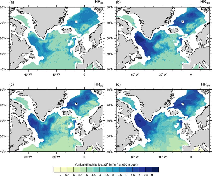
2320                                          O. Gutjahr et al.: Comparison of ocean vertical mixing schemes in MPI-ESM1.2

Table 1. Overview of the 100-year long control simulations conducted with MPI-ESM1.2-HR. All simulations use a T127 (about 100 km)
resolution in the atmosphere and a resolution of 0.4◦ (about 40 km) on a tripolar grid (TP04) in the ocean. The number of vertical levels is
95 in the atmosphere and 40 in the ocean, respectively. All models were analysed for model years 81–100.

    Experiment   Ocean mixing scheme   Description                                                         Reference
    HRpp         PP                    reference simulation                                                Pacanowski and Philander (1981)
    HRkpp        KPP                   uses PP scheme below mixed√layer                                    Large et al. (1994), Griffies et al. (2015)
    HRtke        TKE                   background diffusivity K = 2Emin /N with Emin = 10−6 m2 s−2         Gaspar et al. (1990)
    HRide        TKE+IDEMIX            Emin = 0 m2 s−2 ; prognostic simulation of internal gravity waves   Eden et al. (2014)

part of the High-Resolution Model Intercomparison Project                   eterize
                                                                                  √ internal wave breaking. Because of the relationship
(HighResMIP; Haarsma et al., 2016).                                         K = 2Emin /N for the background diffusivity in the TKE
   The third experiment (HRtke ) used the TKE scheme with                   scheme (see Appendix A3), HRtke simulates a small K in
a background diffusivity that depends on the buoyancy fre-                  the tropical and subtropical ocean, where N is positive, and a
quency and on a minimum value for TKE (see Appendix A3)                     large K in the high-latitude ocean, where N is negative. Even
but without any contribution from IDEMIX. In the last ex-                   more heterogeneous is the distribution of K in HRide , which
periment (HRide ), we used the TKE scheme together with                     simulates stronger mixing above rough topography and mix-
IDEMIX (TKE+IDEMIX) and replaced the artificial back-                       ing coefficients of about 2 orders of magnitude lower above
ground diffusivity with one diagnosed from TKE that is fu-                  the abyssal plains and in the Arctic Ocean. Hotspots of strong
elled by the internal wave dissipation (see Sect. A3 for more               vertical mixing are simulated for all four cases particularly in
details). If not explicitly mentioned, we used default values               the subpolar North Atlantic (SPNA), in the Nordic Seas, and
for the parameters of the mixing schemes, as listed in the re-              in the Weddell and Ross seas of the Southern Ocean. Exces-
spective original description (see also Appendix A), without                sive deep convection in the Weddell Sea is a known issue in
analysing the effect of changed parameters.                                 ocean models (e.g. Sallée et al., 2013; Kjellsson et al., 2015;
   The initial state was derived from a MPI-ESM1.2-HR sim-                  Heuzé et al., 2015; Naughten et al., 2018) and not unique
ulation (with the PP scheme) that was nudged to the aver-                   to MPI-ESM1.2-HR. The unrealistic convection is related
aged temperature and salinity state of 1950 to 1954 of the                  to anomalously frequent open-ocean Weddell Sea polynyas
Met Office Hadley Centre EN4 observational data set (ver-                   (Gordon, 1978; Carsey, 1980; Gordon, 2014). HRide reduces
sion 4.2.0; Good et al., 2013), as described in Gutjahr et al.              the occurrence of this spurious deep convection, which we
(2019). All simulations were forced by constant 1950s condi-                will discuss in Sect. 4.4.
tions according to the HighResMIP protocol (Haarsma et al.,                    A closer look at Fig. 1 reveals more regional differences in
2016). As recommended in this protocol, the model was not                   the above-mentioned areas. We will relate them to biases in
retuned to obtain isolated effects from changing the ocean                  temperature and salinity (Sect. 3.2 and 3.4) and discuss them
vertical mixing scheme. If not stated otherwise, we analysed                in more detail for the SPNA and Nordic Seas (Sect. 4.1), the
averages over the last 20 model years (model years 81 to                    Fram Strait (Sect. 4.2), the Arctic Ocean (Sect. 4.3), and the
100). Although our focus is on the ocean, we briefly present                Southern Ocean (Sect. 4.4).
results for the atmosphere as well.
                                                                            3.2    Sea surface temperature and salinity bias
3     Effects on the global ocean
                                                                            The sea surface temperature (SST) is a key quantity for
In the following, we present how the choice of the ocean ver-               the atmosphere–ocean coupling. Reducing biases of SST in
tical mixing scheme affects the ocean mean state in control                 model simulations is thus of crucial importance. However,
simulations with MPI-ESM1.2-HR. We first present results                    the causes of SST biases are often complex and result, among
for the global ocean before discussing specific regional as-                others, from insufficient horizontal and vertical resolution
pects in Sect. 4.                                                           and from the need to parameterize subgrid-scale processes,
                                                                            which has the largest influence on the biases (Fox-Kemper
3.1     Spatial distribution of vertical diffusivity                        et al., 2019). Vertical mixing is thereby only one of these pa-
                                                                            rameterizations.
Figure 1 shows the spatial distribution of the vertical diffusiv-              Overall, the SSTs are mostly colder in the MPI-ESM1.2-
ity K for the model layer at 1020 m depth. Apart from bound-                HR simulations compared with EN4 (Fig. 2). Although ver-
ary flows, deep convection regions, and the surface mixed                   tical mixing has little effect on the SST bias in large parts of
layer, K is approximately homogeneous in the simulations                    the ocean, some areas are more sensitive. One such area is the
with PP and KPP. Both simulations use a simple constant                     North Atlantic with its subpolar gyre, as well as the Nordic
background diffusivity of K = 1.05×10⁻⁵ m2 s−2 to param-                    Seas. The largest cold bias occurs in the North Atlantic and

Geosci. Model Dev., 14, 2317–2349, 2021                                                        https://doi.org/10.5194/gmd-14-2317-2021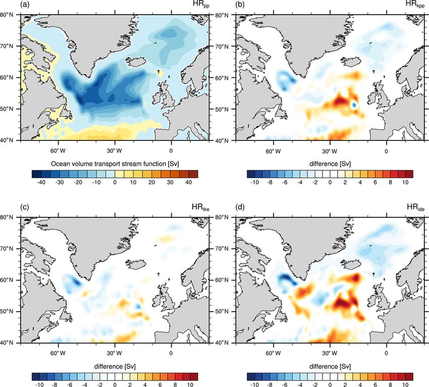
O. Gutjahr et al.: Comparison of ocean vertical mixing schemes in MPI-ESM1.2                                                   2321

Figure 1. Time-averaged vertical diffusivity log10 (K) (m2 s−1 ) at a depth of 1020 m in the MPI-ESM1.2-HR simulations for (a) HRpp ,
(b) HRkpp , (c) HRtke , and (d) HRide .

amounts to −7 ◦ C in HRpp . This cold bias is a common phe-          yet well understood. Most likely it is linked to the reduced
nomena in ocean models (e.g. Randall et al., 2007) and is            sea ice formation that we will discuss in the next section.
mainly caused by a too-zonal pathway of the Gulf Stream
(Dengg et al., 1996) in relation to insufficient horizontal res-     3.3   Sea ice
olution and northward heat transport (Wang et al., 2014). By
using a vertical mixing scheme other than PP, we find that the       The extent and thickness of sea ice in March in the Arc-
SST cold bias in the North Atlantic is reduced (Fig. 2b–d).          tic Ocean and the Nordic Seas are shown in Fig. 4. We
This reduction of the cold bias can be explained by a gener-         compare the sea ice thickness to average thickness (1979–
ally warmer North Atlantic. A stronger Atlantic meridional           2005) of the Pan-Arctic Ice-Ocean Modeling and Assimi-
overturning circulation (AMOC) in the simulations with KPP           lation System (PIOMAS) reanalysis (Zhang and Rothrock,
and TKE (see Sect. 3.5) transports more heat northwards that         2003; Schweiger et al., 2011). We define the ice edge as the
leads to warmer temperatures in the SPNA, especially in the          15 % ice concentration and compare it with the European
Labrador and Irminger seas, and in the Nordic Seas.                  Organisation for the Exploitation of Meteorological Satel-
   Strong warm biases occur also in the tropical upwelling re-       lites (EUMETSAT) Ocean and Sea Ice Satellite Applica-
gions off the west coasts of Africa and South America, which         tion Facility (OSI SAF) (OSI-409-a; v1.2) product (1979–
are related to insufficiently resolved coastal winds that force      2005) (EUMETSAT Ocean and Sea Ice Satellite Application,
the upwelling of colder water (Milinski et al., 2016).               2015).
   The sea surface salinity is mostly unaffected by the chosen          The ice extent is largest in the reference simulation with
vertical mixing scheme, except in the Arctic Ocean (Fig. 3)          the PP scheme (Fig. 4a). The ice edge extends further south
and in the western and eastern equatorial Pacific, which could       everywhere than in PIOMAS, especially in the Nordic Seas
be related to differences in the feedback with the atmosphere.       and the Labrador Sea. The ice edge in the Labrador Sea and
By using the TKE or TKE+IDEMIX scheme, the salinity                  the Nordic Seas lies further north in the simulations with KPP
bias is considerably reduced, especially in the Canada Basin         and TKE(+IDEMIX), especially in HRide . In the North Pa-
(Fig. 3c–d). The cause for these fresher surface waters is not       cific, the ice edge is less affected and lies only further north
                                                                     in the Sea of Okhotsk in HRide . The more northerly location
                                                                     of the ice edge in the KPP and TKE(+IDEMIX) simulations

https://doi.org/10.5194/gmd-14-2317-2021                                               Geosci. Model Dev., 14, 2317–2349, 2021
2322 O. Gutjahr et al.: Comparison of ocean vertical mixing schemes in MPI-ESM1.2
Figure 2. Time-averaged sea surface temperature bias of MPI-ESM1.2-HR minus EN4 (1945–1955) for (a) HRpp , (b) HRkpp , (c) HRtke ,
and (d) HRide .
than in HRpp results from warmer water temperatures in the model layer at 740 m depth (Fig. 6). Exceptions are the
Nordic Seas and Labrador Sea, which causes the sea ice to Southern Ocean and parts of the North Atlantic, where the
retreat. ocean is colder at upper to intermediate depth. In the Atlantic
Ice thickness is lower in all simulations compared to PI- Ocean, the warm biases are mainly linked to the representa-
OMAS, especially in the central Arctic and north of Green- tion of the Agulhas Current system and Mediterranean Over-
land, and lowest in HRide . What causes thinner ice in the flow Water (MOW), as well as to the pathway of the Gulf
simulations with KPP and TKE(+IDEMIX) is unclear and Stream. Previous studies with MPI-ESM1.2 have shown that
remains for further investigation. It could be related to lower these warm biases diminish with increasing spatial resolu-
ice production in the marginal seas, especially in the Laptev tion (Gutjahr et al., 2019; Putrasahan et al., 2019). Advec-
Sea, and could require further tuning of the lead-close pa- tion of these warmer (and more saline) water masses causes
rameterization. subsequent warm biases in the SPNA, Nordic Seas, and Arc-
In the Southern Hemisphere, there is also thinner ice sim- tic Ocean. Even though an eddy-resolving resolution (0.1◦ )
ulated with the TKE and TKE+IDEMIX scheme for the reduces most of these biases, as shown by Gutjahr et al.
time-averaged September (Fig. 5), especially along the coast (2019) with MPI-ESM1.2-ER, the choice of the vertical mix-
of Antarctica. However, we note a closed sea ice cover in ing scheme also affects the hydrographic biases; for instance,
the Weddell Sea in HRide that reduces spurious convec- with TKE+IDEMIX, the warm bias is reduced in the Arctic
tion within the Weddell Sea polynya (see more details in Ocean but enhanced for the MOW (Fig. 6).
Sect. 4.4.1). The sea ice extent is larger than in OSI SAF Salinity shows a similar bias pattern at intermediate depth
but differs only slightly between the simulations. (Fig. 7). The Atlantic is too saline, which is again due to
the poor representation of the MOW and the Agulhas Cur-
3.4 Ocean interior rent system. Consequently, northward advection by the Gulf
Stream and the boundary currents along the European shelf
3.4.1 Horizontal maps of hydrographic biases distribute these saline waters into the SPNA and Nordic Seas,
where they affect the local water masses (Reid, 1979; Mc-
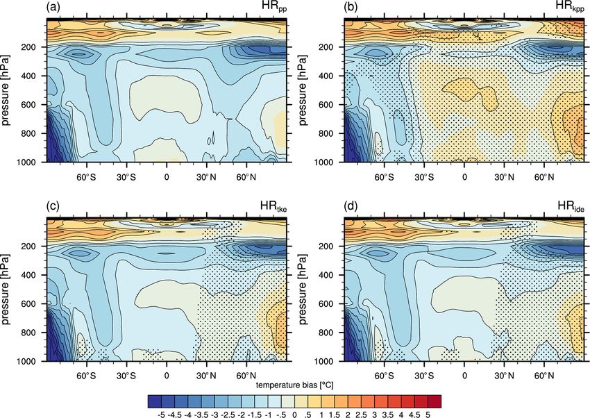
At intermediate depth, all simulations are too warm com- Cartney and Mauritzen, 2001; Lozier and Sindlinger, 2008).
pared to EN4, as shown by the temperature bias for the
Geosci. Model Dev., 14, 2317–2349, 2021 https://doi.org/10.5194/gmd-14-2317-2021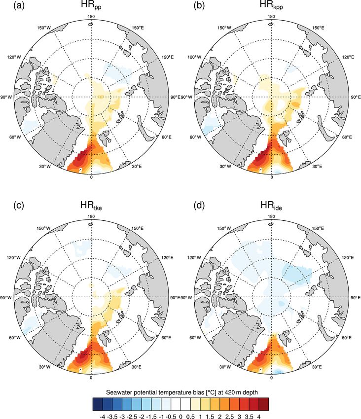
O. Gutjahr et al.: Comparison of ocean vertical mixing schemes in MPI-ESM1.2                                                 2323

Figure 3. Time-averaged sea surface salinity bias of MPI-ESM1.2-HR minus EN4 (1945–1955) for (a) HRpp , (b) HRkpp , (c) HRtke , and
(d) HRide .

At a resolution of 0.4◦ , MPI-ESM1.2-HR is unable to capture         diffusivity becomes very low (O(10−6 m2 s−2 )). We specu-
the Agulhas Retroflection. Although all simulations show a           late that this lower diffusivity reduces mixing with the over-
similar salinity bias in the Agulhas region, we note a larger        lying, less saline North Atlantic Central Water, so that the
bias for HRkpp , HRtke , and HRide . This larger bias indi-          warm, highly saline core of the MOW is less diluted than in
cates a stronger inflow of warm and salty water from the In-         the other simulations. However, the MOW is already saltier
dian Ocean. In fact, the inflow is about 10 Sv stronger with         by about 0.4 psu and 0.5 ◦ C warmer before it flows into the
TKE(+IDEMIX) and about 15 Sv with KPP than the 40 to                 Atlantic. It remains a subject of further investigation what
50 Sv in HRpp (Fig. 8). We further notice a large salinity bias      causes this warmer and saltier MOW in TKE+IDEMIX. Pos-
in all simulations in the South Pacific that seems to be linked      sibly, the scheme modifies the variability of the near-surface
to the South Pacific gyre. We speculate that the bias is due         wind field or the net evaporation over the Mediterranean Sea
to unresolved eddies in the East Australian Current and pro-         (Aldama-Campino and Döös, 2020).
cesses at the border zone of the South Pacific Current and              We further note a slight freshwater bias in the Arctic
the Subantarctic Front. A more detailed analysis is needed to        Ocean in HRide that we will describe in relation to the At-
identify the cause of this model bias, which we suspect to be        lantic Water layer in Sect. 4.2.
related to model resolution but will not explore here.
   The largest difference in salinity bias is linked to the repre-   3.4.2   Vertical sections through the Atlantic and Arctic
sentation of MOW. Although all models produce warmer and                     oceans
more saline MOW, the bias is decreased only in HRtke . The
bias even becomes considerably larger when TKE is used               A vertical section of the zonally averaged potential temper-
with IDEMIX instead of an artificial background diffusiv-            ature bias through the Atlantic and Arctic Oceans (Fig. 9)
ity (Fig. 7d). Although the use of IDEMIX increases vertical         shows predominantly too-cold near-surface water, especially
eddy diffusivity at the overflow sill of the Strait of Gibraltar     in the North Atlantic, where the cold bias extends to a depth
and in the Gulf of Cádiz (not shown), downstream vertical            of about 1000 m due to errors in heat convergence resulting
mixing over the abyssal plains of the Atlantic is very low,          from a misrepresented Gulf Stream and North Atlantic Cur-
probably due to the low internal wave activity, so that the          rent. The intermediate water masses are too warm compared
                                                                     with EN4 and there appears almost no bias in the deeper

https://doi.org/10.5194/gmd-14-2317-2021                                               Geosci. Model Dev., 14, 2317–2349, 2021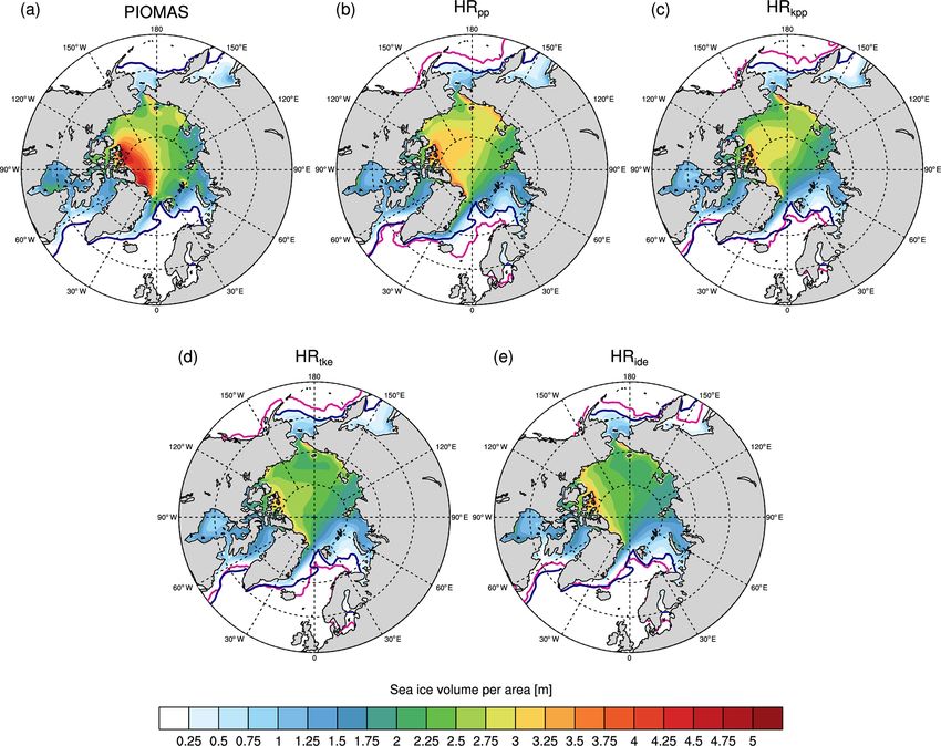
2324                                     O. Gutjahr et al.: Comparison of ocean vertical mixing schemes in MPI-ESM1.2

Figure 4. Time-averaged Arctic sea ice thickness in March for (a) PIOMAS reanalysis (March 1979–2005; Zhang and Rothrock, 2003;
Schweiger et al., 2011), (b) HRpp , (c) HRkpp , (d) HRtke , and (e) HRide . The 15 % sea ice concentration of the EUMETSAT OSI SAF
(averaged over March 1979–2005) is contoured in dark blue and those of the simulations in magenta.

ocean, since the simulation length is too short to affect the         These already-too-warm waters are transported north
abyssal ocean. This general bias pattern is established in all     throughout the whole Atlantic and eventually reach the
simulations, but we note some differences.                         SPNA and Nordic Seas. Part of it continuous further into the
   All simulations simulate a too-warm (and saline) inflow         Arctic Ocean at a depth of 500 m to more than 1000 m, where
from the Indian Ocean to the South Atlantic, roughly at            it becomes the Atlantic Water (AW) layer, which is roughly
30◦ S. The model resolution is too coarse to correctly capture     1 ◦ C warmer than in EN4. Due to stronger recirculation in
the Agulhas Current system; in particular, the retroflection       Fram Strait (see Sect. 4.2), less AW enters the Arctic Ocean
and Agulhas rings are not well represented. Instead, warm          in HRide , reducing the warm bias.
and saline water flows more or less constantly from the In-           In the Nordic Seas, the water temperature is higher in all
dian Ocean into the South Atlantic. From all simulations, this     simulations with KPP and TKE(+IDEMIX) than in HRpp .
misrepresentation is strongest in HRide . The reason for this      Although the higher temperature partly compensates for the
behaviour remains a subject for future studies.                    increase in salinity, the overflows across the Greenland–
   A second source of too-warm water is related to the MOW,        Iceland–Scotland Ridge are dense enough and reach depths
as described above. The core of the MOW reaches a neu-             of about 3000 m. Their warmer temperature can be seen at
tral buoyancy surface slightly above 1000 m depth at roughly       and south of 60◦ N. Similarly, also the deep water formed in
30◦ N. The MOW is warmest in HRide but colder in HRtke             the Labrador Sea is warmer than in HRpp and together these
compared to the reference simulation.                              water masses cause a warm bias when exported as the Deep
                                                                   Western Boundary Current.

Geosci. Model Dev., 14, 2317–2349, 2021                                             https://doi.org/10.5194/gmd-14-2317-2021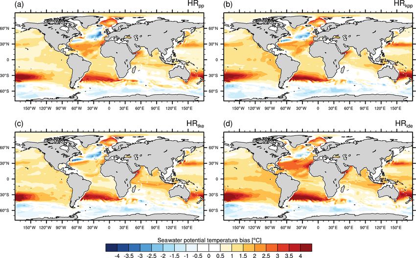
O. Gutjahr et al.: Comparison of ocean vertical mixing schemes in MPI-ESM1.2                                                             2325

Figure 5. Time-averaged Arctic sea ice thickness in March for (a) HRpp , (b) HRkpp , (c) HRtke , and (d) HRide . The 15 % sea ice concentration
of the EUMETSAT OSI SAF (averaged over March 1979–2005) is contoured in dark blue and those of the simulations in magenta.

   Salinity shows a similar bias pattern (not shown) with too-            of > 18 Sv at 26.5◦ N (Fig. 10) compared with about 15 Sv
saline waters where there is a warm bias.                                 in HRpp . A stronger upper cell may imply a stronger north-
                                                                          ward heat transport, whereas a deeper upper cell indicates
3.5   AMOC and transport                                                  a stronger southward transport of NADW (see Sect. 4.1.2).
                                                                          To compensate for the increased overturning in the Nordic
                                                                          Seas, the water in the Atlantic must be replaced by a stronger
The SPNA and the Nordic Seas are important regions for the
                                                                          inflow from the Indian Ocean, which is the case in the simu-
global climate, where the vertical connection between the up-
                                                                          lations with KPP and TKE(+IDEMIX), as seen in Fig. 8.
per warm and the lower cold branch of the AMOC is estab-
                                                                             We note, however, that the bottom cell is weaker in all sen-
lished. The northward-flowing warm AW is cooled by ex-
                                                                          sitivity simulations, which is probably due to a stronger mix-
tensive heat loss to the atmosphere until it becomes dense
                                                                          ing of NADW with Antarctic Bottom Water (AABW), caus-
enough to sink into deeper layers. Together with the dense
                                                                          ing the latter to vanish further south. The simulation length
overflow water from the Nordic Seas, it leaves the SPNA
                                                                          of 100 years is too short to see pronounced effects in the
as North Atlantic Deep Water (NADW) with the southward-
                                                                          deep ocean, but it could be expected that over longer periods
flowing Deep Western Boundary Current (DWBC).
                                                                          (several centuries) the additional mixing from internal waves
   The simulations with KPP and TKE(+IDEMIX) produce
a stronger and deeper-reaching upper branch of the AMOC

https://doi.org/10.5194/gmd-14-2317-2021                                                      Geosci. Model Dev., 14, 2317–2349, 2021
2326                                        O. Gutjahr et al.: Comparison of ocean vertical mixing schemes in MPI-ESM1.2

Figure 6. Time-averaged potential temperature bias of MPI-ESM1.2-HR minus EN4 (1945–1955) at a depth of 740 m for (a) HRpp ,
(b) HRkpp , (c) HRtke , and (d) HRide .

might affect the diapycnal diffusion of the upwelling deep           why we expect differences in vertical diffusion and mixed
water, e.g. in the Pacific.                                          layer depths (MLDs). Eddies are only partially resolved in
                                                                     MPI-ESM1.2-HR, so we do not expect the exchange of deep
                                                                     water with the boundary currents to be realistic.
4     Effects on the regional ocean                                     The largest diffusivities (K) are simulated in the Labrador
                                                                     Sea and the Nordic Seas (Fig. 11), with markedly greater
In this section, we discuss some regional areas in more detail,      values in the simulations with KPP and TKE(+IDEMIX).
in particular the Atlantic Ocean, the Nordic Seas and Fram           In particular, we note increased vertical diffusivities in the
Strait, the Arctic Ocean, and the Southern Ocean. We already         Irminger Sea, where open-ocean deep convection occurs and
note here that the insufficient model resolution determines          contributes to the formation of Labrador Sea water (e.g.
the large-scale bias pattern, as shown by Gutjahr et al. (2019).     Pickart et al., 2003; Våge et al., 2011).
                                                                        In the PP scheme, the vertical instability is parameterized
4.1     Subpolar North Atlantic and the Nordic Seas                  by enhancing the diffusivity to K = 0.1 m2 s−1 . The con-
                                                                     vection parameterization in KPP is more complex, where
4.1.1    Convection and mixed layer depths                           non-local transport terms (see Appendix A2) redistribute the
                                                                     surface fluxes throughout the ocean surface boundary layer.
The sinking of buoyant Atlantic Water is thought to be es-           These non-local transport terms depend on the net heat and
tablished by downwelling of dense water along the bound-             freshwater fluxes at the ocean surface, on K, and on a dimen-
ary currents with complex interplay of deep convection and           sionless vertical shape function (Large et al., 1994; Griffies
the mesoscale eddy field (e.g. Katsman et al., 2018; Brügge-         et al., 2015).
mann and Katsman, 2019; Sayol et al., 2019; Georgiou et al.,            In the TKE scheme, the buoyancy term (third term on the
2019). The water mass transformation of Atlantic Water oc-           right-hand side of Eq. A15), which usually is an energy trans-
curs, however, in areas of deep convection and lateral ex-           fer from TKE to mean potential energy, acts in this case
change with the boundary current by eddies. Convection, or           (N 2 < 0) in the opposite direction and enhances TKE. How-
vertical instability, is parameterized differently in the vertical   ever, besides differences in the parameterizations, remotely
mixing schemes in MPI-ESM1.2 (see Appendix A), which is

Geosci. Model Dev., 14, 2317–2349, 2021                                              https://doi.org/10.5194/gmd-14-2317-2021
O. Gutjahr et al.: Comparison of ocean vertical mixing schemes in MPI-ESM1.2 2327
Figure 7. Time-averaged salinity bias of MPI-ESM1.2-HR minus EN4 (1945–1955) at a depth of 740 m for (a) HRpp , (b) HRkpp , (c) HRtke ,
and (d) HRide .
changed water mass properties, and hence density changes, with KPP and TKE(+IDEMIX), the strength of the gyres is
also affect convection and the MLD in the SPNA. Therefore, stronger than in HRpp (Fig. 13). This enhanced updoming is
it is not straightforward to diagnose what is a cause and what caused by a combination of a more saline SPNA and Nordic
is a consequence for changes in the MLDs. Seas, e.g. about +0.2 psu in the Greenland Sea, and enhanced
The average MLDs in March are shown in Fig. 12. A direct heat loss in the gyre centres. The steeper isopycnal gradients
comparison with MLDs derived from Argo floats is not op- accelerate the geostrophic flow around the convection cen-
timal, because our simulations are control simulations with tres leading to a roughly 10 Sv stronger boundary current in
1950s greenhouse gas forcing. Keeping this in mind, we find the Labrador Sea and a Greenland gyre that is about 5 Sv
profound differences to Argo-float-derived MLDs and across stronger.
the simulations. As with vertical diffusivity, all simulations
show the deepest mixed layers in the Labrador Sea and a 4.1.2 Overflows from the Nordic Seas
second maximum in the Greenland–Iceland–Norway (GIN)
seas. In general, KPP and TKE(+IDEMIX) tend to simu- A substantial contribution to the NADW constitutes the Den-
late deeper mixed layers. In the Labrador Sea, the convection mark Strait overflow water (DSOW; σ > 1027.8 kg m−3 ),
area extends too far north in all simulations due to the lack of which accounts for about half of the observed overflows
mesoscale eddies that would impede convection by restrat- from the Nordic Seas (Hansen et al., 2004), being its dens-
ification of the water column (e.g. Eden and Böning, 2002; est water mass. The other major overflow pathway across
Brüggemann and Katsman, 2019; Gutjahr et al., 2019). HRide the Greenland–Iceland–Scotland Ridge is through the Faroe–
simulates deeper mixed layers in the centre of the Greenland Shetland Channel (FSC; σ > 1027.75 kg m−3 ) and through
Sea gyre and particular around Jan Mayen, which might be the Faroe Bank Channel (FBC; σ > 1027.75 kg m−3 ).
caused by internal wave activity, especially along the Kol- The increased MLDs in the simulations with KPP and
beinsey and Mohn ridges and along the Jan Mayen Fracture TKE(+IDEMIX) due to stronger deep convection in the
Zone. Nordic Seas suggest higher overflow volumes. We applied
Due to stronger updoming of the isopycnals in the Welch’s two-sided t tests with α = 0.05 (n = 20) to test for
Labrador, Irminger, and Greenland seas in the simulations significant differences in the simulated overflows. See Ta-
ble A1 for all test results.
https://doi.org/10.5194/gmd-14-2317-2021 Geosci. Model Dev., 14, 2317–2349, 20212328 O. Gutjahr et al.: Comparison of ocean vertical mixing schemes in MPI-ESM1.2 Figure 8. Time-averaged, vertically integrated volume transport in the Agulhas region south of Africa as simulated by MPI-ESM1.2 (a) HRpp and the difference (experiment minus HRpp ) for (b) HRkpp , (c) HRtke , and (d) HRide . First, we note that all simulations underestimate the ob- served 2.2 Sv by Hansen et al. (2016). The deviations be- served DSOW volume transport of about 3.2 to 3.4 Sv by tween the models are of the order of 10 %, with a higher roughly 1 Sv (see Table 2). Compared with HRpp , how- mean transport in HRtke (p < 0.01) and a lower transport in ever, we find about 10 % to 20 % higher DSOW transport in HRide (p < 0.01). HRkpp , HRide and especially in HRtke (all with p < 0.01). Overall, these results suggest about 10 % higher overflow The transport in the KPP and TKE simulations, however, is transported across the Greenland–Iceland–Scotland Ridge does not differ significantly (p values of 0.13 to 0.52). The with KPP and TKE, which contributes to a stronger upper higher amount of DSOW might thus explain at least partly cell of the AMOC. the stronger upper cell of the AMOC and in particular the AMOC strength around 60◦ N. 4.2 Fram Strait and Atlantic Water layer Although they are overestimated compared to the obser- vations, the FSC overflows in the simulations are of simi- AW is the main supplier of salt and oceanic heat to the Arc- lar magnitude (3.2 to 3.3 Sv), with the exception of HRtke , tic Ocean. From the Nordic Seas, it flows northwards into which produces an approximately 10 % higher (3.5 Sv) over- Fram Strait, where about half of the AW recirculates south- flow transport (p < 0.01). The FBC overflows are about 15 % wards between 76 and 81◦ N and becomes part of the East to 20 % lower in the models (1.7 to 1.9 Sv) than the ob- Greenland Current. A smaller fraction continues northward Geosci. Model Dev., 14, 2317–2349, 2021 https://doi.org/10.5194/gmd-14-2317-2021
O. Gutjahr et al.: Comparison of ocean vertical mixing schemes in MPI-ESM1.2                                                            2329

Figure 9. Zonal-mean potential temperature bias of MPI-ESM1.2-HR minus EN4 (1945–1955) in the Atlantic and Arctic Ocean for (a) HRpp ,
(b) HRkpp , (c) HRtke , and (d) HRide .

Table 2. Time-averaged volume transport (1 Sv= 106 m3 s−1 ) of Denmark Strait overflow water (DSOW), Faroe Bank Channel (FBC), and
Faroe–Shetland Channel (FSC) overflow from simulations with MPI-ESM1.2-HR. Hansen et al. (2017) note that measurements by Rossby
and Flagg (2012) and Childers et al. (2014) include a closed circulation on the Faroe Shelf (0.6 Sv) and flow on the Scottish Shelf, which are
not included in measurements by Berx et al. (2013) and Hansen et al. (2015). A standard deviation based on annual averages is given for the
simulations.

                               Observations/experiment                    DSOW          FBC          FSC
                               Jochumsen et al. (2017)                    −3.2 ± 0.5    –            –
                               Jochumsen et al. (2012)                    −3.4          –            –
                               Hansen et al. (2016)                       –             2.2          –
                               Berx et al. (2013), Hansen et al. (2015)   –             –            2.7
                               Rossby and Flagg (2012)                    –             –            0.9
                               Childers et al. (2014)                     –             –            1.5
                               HRpp                                       −1.8 ± 0.2    1.8 ± 0.1    3.2 ± 0.4
                               HRkpp                                      −2.1 ± 0.4    1.8 ± 0.2    3.3 ± 0.3
                               HRtke                                      −2.2 ± 0.3    1.9 ± 0.1    3.5 ± 0.2
                               HRide                                      −2.1 ± 0.3    1.7 ± 0.1    3.3 ± 0.3

as the West Spitsbergen Current (WSC). Due to the succes-                 et al., 2007; Shu et al., 2019). This error is thought to be
sive cooling in its path, the subsiding AW flows into the Arc-            related to model resolution and to vertical mixing parame-
tic Ocean at mid-depth with its core at about 400 m depth,                terizations, in particular to the choice of the background dif-
sealed off from the atmosphere by overlying cold polar sur-               fusivity (Zhang and Steele, 2007; Liang and Losch, 2018).
face water.                                                               In terms of model resolution, it was recently shown that a
   A common error of many state-of-the-art ocean models                   high-resolution ocean (0.1◦ or better) reduces biases of the
is an anomalously thick and deep AW layer (e.g. Holloway                  AW layer (Wang et al., 2018; Gutjahr et al., 2019), because

https://doi.org/10.5194/gmd-14-2317-2021                                                     Geosci. Model Dev., 14, 2317–2349, 2021
2330 O. Gutjahr et al.: Comparison of ocean vertical mixing schemes in MPI-ESM1.2
Figure 10. Eulerian stream function (Sv = 106 m3 s−1 ) of the AMOC in depth space simulated by MPI-ESM1.2 (a) HRpp , (b) HRkpp ,
(c) HRtke , and (d) HRide .
eddies are (partly) resolved that also improve the circulation to the stronger Greenland Sea gyre (Chatterjee et al., 2018;
(Wekerle et al., 2017). MPI-ESM-HR at eddy-permitting res- Muilwijk et al., 2019). This contradiction can be explained
olution produces a too-warm AW layer, as shown by Gutjahr by a stronger recirculation of AW in HRide in Fram Strait,
et al. (2019). Here, we demonstrate that this warm bias is which means that less AW flows in the Arctic Ocean and
reduced by using TKE+IDEMIX, which is due to a combi- thus there is less heat.
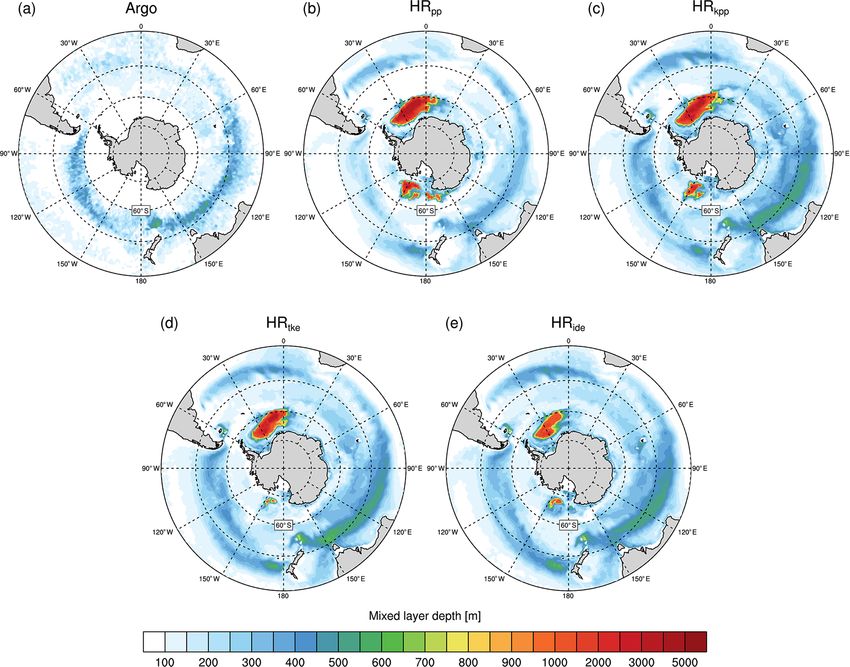
nation of remote (already colder inflowing AW into the Fram Beside this remote effect, there are local effects related to
Strait) and local effects (stronger southward recirculation in enhanced mixing at the YP. A comparison of K of the model
the Fram Strait and stronger heat loss due to enhanced mix- layer at 450 m depth (Fig. 15) shows that the mixing near the
ing). YP in HRide is slightly stronger (Fig. 15d). Internal waves
In HRpp , HRkpp , and HRtke , the warm bias of the AW break near the YP and thus transfer energy to small-scale
layer is about +2 ◦ C at the Yermak Plateau (YP), a bathy- turbulence. This effect is larger in the prognostic IDEMIX
metric feature northwest of the Svalbard archipelago known than from the assumed constant background diffusivity. The
as a hotspot for internal wave activity (see also Fig. A2b) increased mixing in the ocean causes more heat loss, as more
and mixing (e.g. Fer et al., 2010; Crews et al., 2019), and warm AW is exposed to the cold atmosphere and thus cools
less further downstream along the shelf break of the Eurasian more efficiently than in the other simulations. In fact, the sen-
Basin (Fig. 14). It seems that a part of the AW also crosses sible heat flux is about 20 to 40 W m−2 larger in HRide than
the Lomonosov Ridge, except in HRide , and spreads into in HRpp (not shown). For comparison, the sensible heat flux
the Markarov and Canada basins, which is not realistic. The is only about 10 to 20 W m−2 stronger in HRkpp and HRtke .
AW is colder in HRide and better agrees with EN4 in the
Eurasian basin, although the central Arctic Ocean becomes 4.3 Arctic Ocean
about 0.5 ◦ C too cold.
Due to stronger heat loss in the Greenland Sea (not Although largely unknown, sparse observations indicate that
shown), the Atlantic Water is already about 1 ◦ C colder in turbulence in the Arctic Ocean is typically weak (Rainville
HRide compared with the other simulations when it reaches and Winsor, 2008; Fer, 2009). The wind stress cannot act
Fram Strait, although warmer AW could be expected due on the sea surface because of the insulating sea ice cover,
which is why the effect of the wind stress on vertical mix-
Geosci. Model Dev., 14, 2317–2349, 2021 https://doi.org/10.5194/gmd-14-2317-2021O. Gutjahr et al.: Comparison of ocean vertical mixing schemes in MPI-ESM1.2 2331 Figure 11. Time-averaged vertical diffusivity log10 (K) (m2 s−1 ) at a depth of 690 m in the subpolar North Atlantic simulated by MPI- ESM1.2 (a) HRpp , (b) HRkpp , (c) HRtke , and (d) HRide . ing decreases quadratically with the sea ice concentration in diffusivity K is up to 2 orders of magnitude smaller (O(10−6 the simulations with PP and KPP (see Appendix A). In addi- to 10−7 m2 s−1 )) in HRide compared to the other simulations tion, brine rejection in the interior Arctic is less effective as (Fig. 15), in which K is mostly at the constant background a mixing mechanism because of the strong stabilizing verti- value (1.05 × 10⁻⁵ m2 s−1 ). cal salinity gradient. Therefore, apart from enhanced mixing Representing this trapping of internal waves is crucial to by episodic shear events, storms during ice-free conditions simulate eddy diffusivities that are more consistent with mi- (Rainville and Woodgate, 2009), mesoscale eddies, or lat- crostructure measurements, which show low eddy diffusiv- eral intrusion along the boundaries, vertical diffusive mixing ities in deep, flat-bottomed basins but elevated diffusivities dominates over turbulent mixing (Fer, 2009). above deep topography (Rainville and Winsor, 2008). The Internal wave activity is almost absent, except above rough low diffusivities in deep basins agree well with observations topographic features. In fact, internal waves are trapped at the from the Barneo ice camp drift, where O(10−6 m2 s−1 ) was place of their origin and do not propagate far into the Arc- measured below the mixed layer in the Amundsen Basin tic Ocean. This trapping occurs because the Arctic Ocean is (Fer, 2009). north of the critical latitude, which is 74.5◦ N for the M2 tide, Lower vertical diffusivity under sea ice in the Arctic Ocean beyond which the Earth’s rotation prohibits freely propagat- might cause denser water to enter the Nordic Seas (Kim et al., ing internal waves. As a result, they dissipate at or very close 2015), which could then lead to denser overflows across the to their source region with properties similar to lee waves Greenland–Iceland–Scotland Ridge and a 14 % stronger up- (Rippeth et al., 2015, 2017). per cell of the AMOC. Indeed, HRide generates higher over- For this reason, there is little or no contribution to small- flow volumes and a 10 % stronger AMOC, but these are prob- scale turbulence in the inner Arctic Ocean in HRide , espe- ably caused more by denser water masses in the Greenland cially in the deep and flat-bottomed Canada Basin. The eddy https://doi.org/10.5194/gmd-14-2317-2021 Geosci. Model Dev., 14, 2317–2349, 2021
2332                                        O. Gutjahr et al.: Comparison of ocean vertical mixing schemes in MPI-ESM1.2

Figure 12. Time-averaged mixed layer depths (m) in March calculated by the density threshold method (σt = 0.03 kg m−3 ) from (a) 1◦ × 1◦
Argo float data (Holte et al., 2017) (mean March from 2000 to 2018) and from MPI-ESM1.2 (b) HRpp , (c) HRkpp , (d) HRtke , and (e) HRide .

Sea. However, we cannot rule out the effect of denser water            2018). Possible explanations are insufficient freshwater sup-
from the Arctic Ocean.                                                 ply (Kjellsson et al., 2015), mainly due to a lack of glacier
   A contrasting example of higher diffusivities in the inner          meltwater (Stössel et al., 2015), and insufficient wind mix-
Arctic Ocean is a distinct band of strong mixing along and             ing in summer (Timmermann and Beckmann, 2004; Sallée
above the Lomonosov Ridge (Fig. 15d). Here, internal waves             et al., 2013; Kjellsson et al., 2015), which causes a high salin-
break immediately after their formation and thus locally in-           ity bias in the mixed layer that erodes the stratification; see
crease the small-scale turbulence, a process that was also di-         a more detailed discussion in Gutjahr et al. (2019). In con-
rectly measured by Rainville and Winsor (2008).                        trast to this view, Dufour et al. (2017) argue that deep con-
   Assuming a constant background diffusivity thus largely             vection in the Weddell Sea does not necessarily lead to an
overestimates the vertical mixing in the Arctic Ocean. Al-             open-ocean polynya, because strong vertical mixing in low-
though the background diffusivity can be artificially reduced          resolution models inhibits the buildup of a subsurface heat
to mimic this low internal wave activity (e.g. Kim et al.,             reservoir that would be necessary for intermittent Weddell
2015; Sein et al., 2018), the very heterogeneous pattern de-           Sea polynyas.
scribed above would not be captured. The combination of                   We do not expect a realistic representation of the Weddell
TKE with IDEMIX is able to reproduce the spatial pattern               Sea polynya in our MPI-ESM1.2-HR 1950s control simula-
and the correct magnitudes. It further provides an energeti-           tions, because they should develop intermittently only un-
cally more consistent solution that should be preferred.               der pre-industrial conditions and grow out from Maud Rise
                                                                       polynyas (de Lavergne et al., 2014; Gordon, 2014; Kurtakoti
4.4     Southern Ocean and Weddell Sea                                 et al., 2018; Campbell et al., 2019; Cheon and Gordon, 2019;
                                                                       Jena et al., 2019), for which high resolution (0.1◦ or better)
4.4.1    Open-ocean convection in the Weddell Sea                      is required (Stössel et al., 2015; Dufour et al., 2017).
         polynya                                                          Although all simulations produce these semi-permanent
                                                                       Weddell Sea polynyas and thus too-deep mixed layers
A well-known problem in ocean modelling is a too-frequent              (Fig. 16), the area of excessive deep convection is reduced in
semi-permanent Weddell Sea polynya caused by false deep                HRide (Fig. 16e). Similarly, too-deep mixed layers are sim-
convection bringing warm Circumpolar Deep Water (CDW)                  ulated in the Ross Sea, except in HRtke , which simulates
close to the surface (Sallée et al., 2013; Kjellsson et al., 2015;     shallower mixed layers without further reduction when us-
Heuzé et al., 2015; Stössel et al., 2015; Naughten et al.,             ing IDEMIX (HRide ). The Weddell Gyre is also linked to

Geosci. Model Dev., 14, 2317–2349, 2021                                                  https://doi.org/10.5194/gmd-14-2317-2021
O. Gutjahr et al.: Comparison of ocean vertical mixing schemes in MPI-ESM1.2 2333 Figure 13. Time-averaged barotropic volume transport stream function (Sv) in the North Atlantic as simulated by MPI-ESM1.2 (a) HRpp , and the differences of “experiment – HRpp ” for (b) HRkpp , (c) HRtke , and (d) HRide . the Antarctic Circumpolar Current (ACC; Orsi et al., 1993; Table 3. Time-averaged volume transport (1 Sv= 106 m3 s−1 ) of Cheon et al., 2019), because it controls the inflow of rel- the Antarctic Circumpolar Current (ACC) through Drake Passage atively warm and saline CDW into the inner Weddell Sea, from observations and simulations with MPI-ESM1.2-HR. possibly eroding the weak stratification and triggering deep convection. The simulated ACC transport through the Drake Experiment Mean Standard deviation Passage (Table 3) is close to the recently observed 173.31 ± Donohue et al. (2016) 173.3 ± 10.7 – 10.7 Sv (Donohue et al., 2016), whereby HRtke achieves the HRpp 161.41 2.14 best estimate with 174 Sv. Simulations with lower convection HRkpp 191.97 2.99 in the Weddell Sea produce lower transport of about 161 to HRtke 174.31 2.63 163 Sv (HRpp and HRide ), whereas HRkpp produces a much HRide 163.54 4.39 higher transport of 192 Sv because of steeper isopycnals due to enhanced convection in the Weddell Sea. Since eddies are not resolved and the GM coefficient is rather low, there is no favour the formation of sea ice, which insulates the ocean or too little eddy compensation to flatten the isopycnals. from further heat loss and thus impedes convection. In HRide , One possible explanation why HRide simulates less con- the average sea ice concentration in September is about 50 % vection in the Weddell Sea is that IDEMIX creates more mix- to 70 % in the Weddell Gyre (not shown), whereas it is con- ing above the shelf, which spreads near-surface freshwater siderably lower in the other simulations with concentrations laterally into the centre of the Weddell Gyre much more effi- of 20 % to 50 %. Furthermore, the ice is also thicker with ciently (not shown). Fresher conditions in the Weddell Gyre IDEMIX compared with the other simulations (Fig. 5d). Al- https://doi.org/10.5194/gmd-14-2317-2021 Geosci. Model Dev., 14, 2317–2349, 2021
2334                                      O. Gutjahr et al.: Comparison of ocean vertical mixing schemes in MPI-ESM1.2

Figure 14. Time-averaged potential temperature bias of MPI-ESM1.2-HR minus EN4 (1945–1955) at a depth of 420 m in the Arctic Ocean
and the Fram Strait for (a) HRpp , (b) HRkpp , (c) HRtke , and (d) HRide .

though the sea ice concentration is still too low, the spurious    (e.g. Sarmiento et al., 2004). It was shown that high reso-
deep convection in the Weddell Sea is reduced with IDEMIX.         lution (0.1◦ ) leads to deeper and thus more realistic MLDs
                                                                   in the DMB (Li and Lee, 2017; DuVivier et al., 2018; Gut-
4.4.2   Deep mixing band in the Southern Ocean                     jahr et al., 2019), but it is thought that fundamental vertical
                                                                   physics are missing in ocean models (DuVivier et al., 2018).
Another challenge for current ocean models is the represen-           Although HRpp reproduces the DMB in the Indian Ocean,
tation of the deep mixing band (DMB; DuVivier et al., 2018),       the mixed layers are too shallow in almost the entire Pacific
which extends from the western Indian Ocean to the eastern         sector (Fig. 16b). KPP and TKE improve the representation
Pacific Ocean and reaches MLDs of more than 700 m (Holte           of the DMB in the Pacific Ocean and simulate deeper mixed
et al., 2017, Fig. 16a). The DMB builds up over the win-           layers, especially in the Indian Ocean. The MLDs are close
ter months and is deepest in September. Subantarctic Mode          to observations (Fig. 16c–e), albeit with a too-wide DMB,
Water (SAMW; McCartney, 1977) forms in the DMB near                which is probably caused by insufficient model resolution,
the Subantarctic Front, just north of the ACC. The SAMW            since it becomes much narrower when an eddy-resolving
acts as an important carbon sink (e.g. Sabine et al., 2004)        model is used (Gutjahr et al., 2019). The choice of a mix-
and it ventilates the mid-deep ocean (e.g. Sloyan and Rintoul,     ing scheme other than PP has little influence on the MLDs,
2001; Jones et al., 2016), replenishing oxygen and nutrients

Geosci. Model Dev., 14, 2317–2349, 2021                                             https://doi.org/10.5194/gmd-14-2317-2021
You can also read