Improving regional air quality predictions in the Indo-Gangetic Plain - case study of an intensive pollution episode in November 2017
←
→
Page content transcription
If your browser does not render page correctly, please read the page content below
Atmos. Chem. Phys., 21, 2837–2860, 2021
https://doi.org/10.5194/acp-21-2837-2021
© Author(s) 2021. This work is distributed under
the Creative Commons Attribution 4.0 License.

Improving regional air quality predictions in the Indo-Gangetic
Plain – case study of an intensive pollution episode in November
2017
Behrooz Roozitalab1,2 , Gregory R. Carmichael1,2 , and Sarath K. Guttikunda3
1 Centerfor Global and Regional Environmental Research, University of Iowa, Iowa City, IA, USA
2 Chemical and Biochemical Engineering, University of Iowa, Iowa City, IA, USA
3 Urban Emissions, New Delhi, India

Correspondence: Behrooz Roozitalab (behrooz-roozitalab@uiowa.edu) and Gregory R. Carmichael
(gcarmich@engineering.uiowa.edu)

Received: 21 July 2020 – Discussion started: 18 August 2020
Revised: 18 November 2020 – Accepted: 13 January 2021 – Published: 25 February 2021

Abstract. The Indo-Gangetic Plain (IGP) experienced an             cal depth (AOD) of 0.58 (±0.4) over November. The model
intensive air pollution episode during November 2017.              AODs were biased high over central India and low over the
Weather Research and Forecasting model coupled to                  eastern IGP, indicating improving emissions in the eastern
Chemistry (WRF-Chem), a coupled meteorology–chemistry              IGP can significantly improve the air quality predictions. We
model, was used to simulate this episode. In order to capture      also found high ozone concentrations over the domain, which
PM2.5 peaks, we modified input chemical boundary condi-            indicates ozone should be considered in future air quality
tions and biomass burning emissions. The Community At-             management strategies alongside particulate matter.
mosphere Model with Chemistry (CAM-chem) and Modern-
Era Retrospective analysis for Research and Applications
Version 2 (MERRA-2) global models provided gaseous and
aerosol chemical boundary conditions, respectively. We also        1   Introduction
incorporated Visible Infrared Imaging Radiometer Suite (VI-
IRS) active fire points to fill in missing fire emissions in the   Ambient air pollution remains a major environmental is-
Fire INventory from NCAR (FINN) and scaled by a factor of          sue, even after significant worldwide efforts starting after the
7 for an 8 d period. Evaluations against various observations      deadly smog of London in 1952. It is the fifth-ranking risk
indicated the model captured the temporal trend very well al-      of death and a major threat to climate and ecosystems (Co-
though missed the peaks on 7, 8, and 10 November. Modeled          hen et al., 2017; Ramanathan and Carmichael, 2008; Sitch
aerosol composition in Delhi showed secondary inorganic            et al., 2007). Air pollution contains many species; particu-
aerosols (SIAs) and secondary organic aerosols (SOAs) com-         late matter (PM) is currently the air pollutant of most con-
prised 30 % and 27 % of total PM2.5 concentration, respec-         cern, especially in developing countries like India. India is
tively, during November, with a modeled OC/BC ratio of             an emerging economy with a burgeoning population that has
2.72. Back trajectories showed agricultural fires in Punjab        accelerated its industrial activities in the last 3 decades, lead-
were the major source for extremely polluted days in Delhi.        ing to widespread air pollution and resulting adverse health
Furthermore, high concentrations above the boundary lay-           effects. There are many Indian cities on the list of most pol-
ers in vertical profiles suggested either the plume rise in the    luted cities of the world (World-Bank, 2018; Guttikunda et
model released the emissions too high or the model did not         al., 2014; WHO, 2016). Studies show that ozone and par-
mix the smoke down fast enough. Results also showed long-          ticulate matter with a diameter of less than 2.5 µm (PM2.5 )
range-transported dust did not affect Delhi’s air quality dur-     are attributed to more than 1 million individual premature
ing the episode. Spatial plots showed averaged aerosol opti-       deaths in India (Cohen et al., 2017; GBD MAPS Working

Published by Copernicus Publications on behalf of the European Geosciences Union.
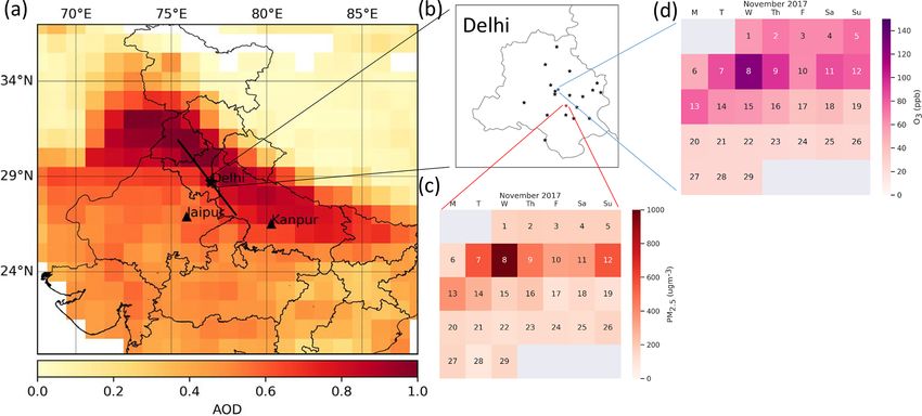
2838                            B. Roozitalab et al.: Improving regional air quality predictions in the Indo-Gangetic Plain

Group, 2018). David et al. (2019) found that anthropogenic         trations measured with the US EPA instrument located at the
emissions within India led to about 80 % of the total prema-       US Embassy in Delhi. Daily PM2.5 concentrations reached
ture deaths due to PM2.5 in India. Furthermore as industrial       values of more than 900 µg m−3 , 15 (37.5) times higher than
activities are growing, emissions are increasing too; health       24 h averaged Indian standards (World Health Organization
impacts attributed to long-term exposure to air pollution are      (WHO) guidelines) (WHO, 2006). However, it is clear that
predicted to increase based on current policies (Conibear et       no day is compliant with the air quality standard values. Af-
al., 2018a).                                                       ter this extreme pollution episode, the Indian government of-
   Short-term extreme pollution events lead to increased hos-      ficially initiated a comprehensive air quality plan called the
pital admissions and mortalities (Anenberg et al., 2018; Ra-       National Clean Air Programme (NCAP) to reduce the air pol-
jak and Chattopadhyay, 2020). Forest and agricultural fires,       lution (MoEF&CC, 2019).
dust storms, increased local activities, and stagnant meteo-          Different groups have studied this period. Dekker et
rological conditions are major contributing factors in these       al. (2019) attributed carbon monoxide (CO) accumulation
air pollution episodes (Beig et al., 2019; Jethva et al., 2018).   between 11 and 14 November to stagnant meteorological
While forecasting models help authorities to notify people         conditions, specifically, to low wind speeds and shallow at-
of these extreme pollution events, hindcasting models help         mospheric boundary layers. Moreover, they argued regional
scientists improve the capabilities of the models to predict       air pollution transport was mostly responsible for this ex-
pollution events, identify the main responsible factors caus-      treme pollution episode (Dekker et al., 2019). However,
ing these events, and inform policy makers as they develop         Beig et al. (2019) concluded biomass burning emissions af-
pollution control strategies. However, the ability of air qual-    ter post-monsoon crop productions, accompanied by long-
ity models for simulating short-term events highly depends         range-transported dust from the Middle East, led to very high
on the quality of input chemical data (i.e., emissions). For       pollution levels although stagnant conditions favored it.
example, the total amount of global fire emissions can dif-           While the current focus of research groups and govern-
fer by a factor of 3–4 based on the emission inventory used        ments is on PM, ozone concentrations also show high values
(Pan et al., 2020). Furthermore, dust storms can travel long       during the post-monsoon season. Figure 1d shows measured
distances and influence another region’s air quality (Ashrafi      daily ozone concentrations at one Central Pollution Control
et al., 2017; Beig et al., 2019). David et al. (2019) attributed   Board (CPCB) station in Delhi; concentrations exceeded In-
about 16 % of total premature PM2.5 -related deaths to emis-       dia’s ozone air quality guidelines. Moreover, the ozone con-
sions outside India. Moreover, studies of black carbon (BC)        centrations followed a similar daily variation to PM during
in southern Asia have revealed that local emissions in west-       November 2017 (Fig. 1d). As a result, extreme pollution
ern India can affect eastern and southern regions’ air qual-       episodes not only cause PM-related health issues but also
ity (Kumar et al., 2015a). As a result, global models, which       increase the risk of chronic obstructive pulmonary disease
provide boundary conditions needed by regional air quality         (COPD) (the most important health outcome of ozone pollu-
models, can significantly affect the simulated results (He et      tion) (Conibear et al., 2018b; US Environmental Protection
al., 2019).                                                        Agency, 2013).
   The Indo-Gangetic Plain (IGP) experiences high levels              Models usually underestimate the concentrations during
of air pollution during the post-monsoon season (October           extreme pollution periods unless they apply chemical data
to early December) due to stagnant meteorological condi-           assimilation (Dekker et al., 2019; Kulkarni et al., 2020; Ku-
tions and higher air pollution emissions (Adhikary et al.,         mar et al., 2015b, 2020). Moreover, there are different in-
2007; Marrapu et al., 2014). Figure 1a shows the averaged          put data in terms of chemical boundary conditions and fire
aerosol optical depth (AOD) retrieved from the Visible In-         emissions that can affect air quality modeling results (He
frared Imaging Radiometer Suite (VIIRS) remote sensing in-         et al., 2019). The main purpose of this study is to inves-
strument during November 2017 over northern India. The             tigate the sensitivity of model predictions to the main in-
IGP region has the highest AOD values with the largest val-        puts into the model. Prediction of extreme pollution events
ues in the northwestern parts, which is mostly due to crop         is important as such events have major impacts on people
residue burning (Beig et al., 2020; Jethva et al., 2018; Liu       and also make a strong impression regarding the capabil-
et al., 2018; Venkataraman et al., 2018; Vijayakumar et al.,       ities of models. However, extreme events are hard to pre-
2016). Kulkarni et al. (2020) found India’s northwestern agri-     dict because they are often heavily impacted by episodic
cultural fires could contribute up to 75 % of Delhi’s PM2.5        emission sources. Here we take the approach of systemati-
concentration.                                                     cally exploring the impacts of different boundary conditions,
   Not only is there significant spatial variation over the        dust, fire, and anthropogenic emissions on the predictions
IGP, but also PM2.5 concentrations change on a daily ba-           of the pollution episode in November 2017. A contempo-
sis (Fig. 1c). Delhi, the capital of India with annual aver-       rary way to try to capture such events in a prediction model
age PM2.5 concentration of 120 µg m−3 (Amann et al., 2017),        is to employ data assimilation (Kumar et al., 2020). The
experienced severe extreme air pollution during Novem-             data assimilation results compensate for deficiencies in the
ber 2017. Figure 1c shows the daily averaged PM2.5 concen-         inputs as well as for structural problems within the mod-

Atmos. Chem. Phys., 21, 2837–2860, 2021                                             https://doi.org/10.5194/acp-21-2837-2021
B. Roozitalab et al.: Improving regional air quality predictions in the Indo-Gangetic Plain                                          2839

Figure 1. WRF-Chem modeling domain, ground measurement stations, and observed air quality: (a) modeling domain and location of Delhi
(∗) and AERONET stations at Jaipur and Kanpur (N) and underlying VIIRS AOD (550 nm) averaged over November 2017; the black line
also shows the path that was used for vertical cross-section analysis. (b) Location of CPCB stations (black stars); US Embassy station (red
star); and North Campus, Delhi University (blue star). (c) Calendar map of averaged daily PM2.5 concentration measured at US Embassy,
(d) Calendar map of averaged daily ozone concentration measured at North Campus, Delhi University.

els. But the effectiveness of data assimilation improves as             2     Methods
the capabilities of the forward model improves. Therefore,
our results are also important for those using data assim-              2.1    WRF-Chem configuration
ilation to improve predictability. In this study, we use the
Weather Research and Forecasting model coupled to Chem-                 WRF-Chem is a numerical modeling framework that solves
istry (WRF-Chem). Through a series of sensitivity experi-               transport, chemistry, and physics of the atmosphere (Grell
ments, we evaluate the impacts of biomass burning emissions             et al., 2005). The online interaction between meteorology,
coming from the Fire INventory from NCAR (FINN) and                     thermodynamic processes, and atmospheric chemistry makes
Quick Fire Emissions Dataset (QFED); chemical boundary                  it a powerful and reliable model in the community. WRF-
conditions retrieved from the Model for Ozone and Related               Chem (version 4.0) with one domain centered on Delhi with
chemical Tracers (MOZART), the Community Atmosphere                     a 15 km horizontal grid resolution and 39 vertical layers was
Model with Chemistry (CAM-chem), the Copernicus Atmo-                   used in this study. The domain was set to be big enough to
sphere Monitoring Service (CAMS), and Modern-Era Ret-                   include the northwest biomass burning and urban emission
rospective analysis for Research and Applications Version 2             sources in the simulation process as they have been shown
(MERRA-2) global models; the role of incorporating VIIRS                to be contributors to poor air quality in the region in pre-
active fire hot spots to improve biomass burning emission in-           vious studies (Amann et al., 2017). In the following, we
ventories and global models to improve chemical boundary                present the model configuration for the base scenario (ID –
conditions; and changes in dust and anthropogenic emissions             FINN_VIIRS_7Xperiod2).
on modeled PM2.5 concentration during November 2017. We                    The National Centers for Environmental Prediction
also evaluate ozone predictions.                                        (NCEP) Global Forecast System (GFS) final analysis (FNL)
   This paper is organized as follows. First, the WRF-Chem              1 × 1◦ and 6 h spatial and temporal resolution meteorologi-
configuration; sensitivity experiments; and the observation             cal fields (https://rda.ucar.edu/datasets/ds083.2/, last access:
datasets, including ground measurements and satellite data,             22 January 2020) were used as initial and boundary condi-
are described. Then, after evaluating the model performance             tions for the meteorology. CAM-chem data (Buchholz, 2019)
for the best experiment, the impacts of using different                 with a horizontal resolution of 0.9 × 1.25◦ and 56 vertical
datasets as input data on modeled PM2.5 concentrations dur-             levels provided chemical boundary conditions for gaseous
ing November 2017 are analyzed and discussed.                           species. MERRA-2 reanalysis data with 0.625 × 0.5◦ hori-
                                                                        zontal and 72 vertical model levels were used for aerosol
                                                                        species (Bosilovich et al., 2016). However, input data have

https://doi.org/10.5194/acp-21-2837-2021                                                  Atmos. Chem. Phys., 21, 2837–2860, 2021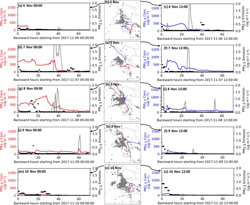
2840                           B. Roozitalab et al.: Improving regional air quality predictions in the Indo-Gangetic Plain

uncertainties, and small uncertainties in nonlinear govern-      dustrialized sources, the literature shows that biomass burn-
ing equations of numerical weather predictions can lead to       ing (e.g. agricultural waste burning) contributes to 37 %
non-negligible errors in results (Xiu, 2010). As a result, re-   of air pollution over the sub-continent (Kumar et al.,
initialization of numerical weather prediction (NWP) mod-        2015a). The Hemispheric Transport of Air Pollution (HTAP
els is suggested instead of free runs (Abdi-Oskouei et al.,      v2.2) (Janssens-Maenhout et al., 2015) emission inven-
2020). In this study, the model ran for 30 h each day start-     tory of 2010 with a 0.1◦ horizontal resolution, mapped to
ing at 00Z and the first 6 h of data was discarded to account    the MOZART–MOSAIC mechanism (https://www2.acom.
for daily spin-up. Meteorological initial and boundary con-      ucar.edu/wrf-chem/wrf-chem-tools-community, last access:
ditions and chemical boundary conditions were re-initialized     1 December 2020), was used as the base anthropogenic
daily at 00Z using global models. However other than for the     emission inventory. Although the accuracy of urban anthro-
first cycle in which global models provided initial chemical     pogenic emission inventories has significant effects on air
conditions data, chemical fields from the previous cycle were    quality modeling studies (Gupta and Mohan, 2015; Kumar
used as the next cycle’s initial chemical conditions. Table 1    et al., 2012; Sharma et al., 2017), the focus of this paper is to
summarizes the WRF-Chem physical and chemical configu-           capture the air pollution due to regional sources; we did not
ration options.                                                  use higher-resolution emission inventories for Delhi.
   Studies have shown improvements for ozone simulations            The Fire INventory from NCAR, version 1.5 (FINNv1.5),
in Delhi using more complicated chemistry mechanisms like        and Model of Emissions of Gases and Aerosols from Nature
MOZART and CBMZ compared to simple mechanisms like               (MEGAN v 2.0.4) were used as biomass burning emission
RACM and RADM (Gupta and Mohan, 2015; Sharma et                  and biogenic emission inventories, respectively (Guenther et
al., 2017). The MOZART gas-phase chemistry mechanism             al., 2006; Wiedinmyer et al., 2011). However, other studies
and the four-bin Model for Simulating Aerosol Interactions       have noticed that uncertainties in FINN emissions can signif-
and Chemistry (MOSAIC-4bin) were used for modeling at-           icantly modify the results (Kulkarni et al., 2020). Therefore,
mospheric chemistry and aerosol properties as suggested          two modifications were applied to FINN data to provide bet-
in previous studies over India (Kumar et al., 2015a). The        ter input data: filling missing fires using VIIRS fire radia-
MOZART version-4 mechanism was initially developed for           tive power (FRP) data and scaling the fire emissions (scaling
global modeling of ozone and other tracers in the troposphere    procedure described in detail later). Liu et al. (2018) used
(Emmons et al., 2010). Although it includes 97 gas-phase         FRP values to approximate the stubble burning areas affect-
and bulk aerosols, all monoterpenes, which are important in      ing Delhi’s air quality. In their statistical study, 99 % of post-
ozone chemistry, were initially lumped together. As a result,    monsoon FRP values were attributed to agricultural fires (Liu
Hodzic et al. (2015) added a detailed treatment of monoter-      et al., 2018). In this study, we used FRP values to improve fire
penes and Knote et al. (2014) updated the isoprene oxida-        emissions. Specifically, we first regridded VIIRS 375 m reso-
tion scheme in the MOZART mechanism in WRF-Chem.                 lution FRP data to our domain. Then at each hour, for all grid
MOSAIC is an aerosol model that considers a wide range           cells that have FINN emissions, we find the corresponding
of aerosol species that are important on a regional scale        mean VIIRS FRP and perform a linear regression between
and treats the chemical and microphysical processes between      FRP and emission flux. Afterwards, we apply the regres-
them including nucleation, coagulation, thermodynamics and       sion line parameters to VIIRS FRP for the grid cells that do
phase equilibrium, and gas–particle partitioning (Zaveri et      not have any FINN emissions, to estimate the flux. It should
al., 2008). Hodzic and Jimenez (2011) updated the secondary      be mentioned that all the available FRP data were utilized
organic aerosol (SOA) formation mechanism, and the up-           disregarding the retrieval’s confidence level. Moreover, we
dated version is available in WRF-Chem for performing re-        used VIIRS instead of MODIS data as they provided higher-
gional air quality modeling studies. MOSAIC-4bin, used in        resolution active fire points data (375 m vs. 1 km), which is
the current study, calculates all the above-mentioned aerosol    an important point for small fires. For example, no active
physics and chemistry in four sectional aerosol size bins with   fire points in the Moderate Resolution Imaging Spectrora-
the assumption that each bin is internally mixed and all the     diometer (MODIS) instrument were reported in 2018 post-
particles within a bin have the same chemical composition        monsoon for Uttar Pradesh (Kulkarni et al., 2020). Figure 9
(Zaveri et al., 2008).                                           shows more fire grid cells in the eastern IGP and central India
   In India, both anthropogenic and natural sources have         when incorporating VIIRS data into the FINN inventory. We
important impacts on air quality. Biomass and biofuel            acknowledge that this technique is a first-order approxima-
use in the residential sector for heating and cooking pur-       tion and can have large errors as FINN is based on burned-
poses make significant contributions to air quality in In-       area algorithms from MODIS-retrieved data; more detailed
dia (Conibear et al., 2018a; David et al., 2019; Venkatara-      research is required to improve the idea.
man et al., 2018). Moreover, there are more than 1000               Dust storms are an important natural pollution source that
power plants and brick kilns in India that are major an-         have caused many pollution events over some parts of India
thropogenic sources of SO2 and particulate matter, respec-       (Kumar et al., 2014a). The Goddard Global Ozone Chem-
tively (Guttikunda and Calori, 2013). Other than these in-       istry Aerosol Radiation and Transport (GOCART) mecha-

Atmos. Chem. Phys., 21, 2837–2860, 2021                                            https://doi.org/10.5194/acp-21-2837-2021
B. Roozitalab et al.: Improving regional air quality predictions in the Indo-Gangetic Plain                                 2841

nism was used to calculate the threshold wind velocity and        FINN_MERRA2). It is important to note that CAMS and
total dust emissions; about 70 % of the total mass was then       MERRA-2 are reanalysis models and use observed data to
distributed between different bins of the other inorganic (OIN    improve the results. CAMS assimilates the MODIS and Ad-
aerosol component in WRF-Chem; OIN represents all pri-            vanced Along-Track Scanning Radiometer (AATSR) satel-
mary inorganic PM) components in the model with the as-           lite instruments’ AODs (Inness et al., 2019). MERRA-2 as-
sumption that the rest are larger than PM10 (Zhao et al.,         similates AOD from multiple sources including MODIS, the
2010). This is based on a study in northern Africa, where         Multi-angle Imaging SpectroRadiometer (MISR), the Ad-
Zhao et al. (2010) allocated about 1 % of the dust to bins with   vanced Very High Resolution Radiometer (AVHRR), and the
a diameter of less than 2.5 µm and 69 % of the dust in bin 4      AErosol RObotic NETwork (AERONET) although assimi-
(2.5–10 µm) and assumed the rest was bigger than 10 µm and        lating some products has been stopped since 2014 (Randles
would not remain in the atmosphere for an influential period.     et al., 2017).
                                                                     Finally, simulations were conducted for various dust emis-
2.2   Sensitivity experiments                                     sion modifications. In one simulation, we turned off the dust
                                                                  emission option in the model (ID – NO_DUST), while in
Three sets of experiments were performed to explore the im-       another simulation, we increased total dust emissions by
pact of using different global data (as either boundary condi-    factor of 5 to explore if dust emissions were underesti-
tions or emissions) and dust emission formulations on PM2.5       mated in the model (ID – DUST_5X). Moreover, we changed
and AOD predictions (Table 2). It should be mentioned that        the allocation of total dust to different bins of the MO-
all the modeling options and other input data remained un-        SAIC module to see whether different allocation of aerosols
changed unless specified.                                         can contribute to the observed extreme pollution in Delhi
   One set of experiments focused on the sensitivity of           (ID – DUST_allocation). Specifically, we took 30 % from
the predictions to biomass burning emissions. First, we           the fourth bin (2.5–10 µm) and allocated 25 % of it to the
compared the impacts of two different biomass burning             third bin (0.625–2.5 µm) and 5 % to the second bin (0.156–
emission inventories, namely FINN and QFED (Koster et             0.625 µm). More allocation to bins 2 and 3 was not consid-
al., 2015). Specifically, simulations using QFED (ID –            ered, as it was not realistic of the large-size nature of dust
QFED_CAMCHEM) and FINN (ID – FINN_CAMCHEM)                        aerosols. The FINN_10Xall scenario represents the simula-
were performed to understand the impact of different fire de-     tion with the turned-on dust option (original allocation) in the
tection algorithms. When using QFED, it should be men-            model. Detailed results from experiments on boundary con-
tioned that we mapped total CO values to VOC species in           ditions and dust emissions can be found in the Supplement.
the MOZART chemistry mechanism based on emission fac-
tors provided in the literature instead of using VOC emis-        2.3   Observation data
sions directly from QFED (Akagi et al., 2011). Second, we
investigated whether FINN fire emissions were underesti-          The model performance was evaluated using ground mea-
mated for all the days (ID – FINN_10Xall), some days (ID –        surements, spaceborne instruments, and global reanaly-
FINN_10Xperiod1), or just 1 d before the pollution episode        sis data. Specifically, we used data collected by the
on 5 November (ID – FINN_10Xday). Then after modify-              CPCB over the domain for performing statistical analy-
ing FINN using VIIRS FRP data, we performed a sensitiv-           sis. They include stations over Delhi (19 stations), Ra-
ity test by changing the period for scaling fire emissions.       jasthan (10 stations), Haryana (4 stations), and Pun-
Specifically, we scaled fire emissions for a 15 d period be-      jab (3 stations). No additional quality control filters,
tween 3 and 17 November (ID – FINN_VIIRS_10Xperiod1)              other than the ones by the CPCB (https://cpcb.nic.in/
and an 8 d period between 5 and 13 November (ID –                 quality-assurance-quality-control/, last access: 20 Febru-
FINN_VIIRS_10Xperiod2). We also evaluated the perfor-             ary 2021), were applied. We evaluated the results after ap-
mance for a scaling factor of 10 in comparison with 7 (ID         plying the filters proposed by other studies (e.g., Kumar et
– FINN_VIIRS_7Xperiod2). Anthropogenic emissions over             al., 2020); they had slight impacts on statistics (shown in
India also have high uncertainties (Saikawa et al., 2017).        the Supplement). PM2.5 data measured by a US EPA instru-
As a result, we studied how increasing the anthropogenic          ment at the US Embassy in Delhi were used as the reference
aerosol emissions by a factor of 2 affects the results (ID –      station data. Level-2 VIIRS remote sensing instrument data
BASE_ANTHRO2X).                                                   on board the Suomi National Polar-orbiting Partnership (S-
   Another set of experiments evaluated the impacts of chem-      NPP) were used for comparing the spatial pattern of AOD
ical boundary conditions. Many global datasets can be used        and fire counts over the domain. Specifically, aerosol prod-
in regional air quality modeling. Simulations were per-           ucts with around a 6 km horizontal resolution based on the
formed using the global modeling systems CAM-chem (ID             Deep Blue algorithm (Hsu et al., 2019) and 375 m active fire
– FINN_CAMCHEM), MOZART (ID – FINN_MOZART),                       products based on the VNP14IMG algorithm (Schroeder et
CAMS (ID – FINN_CAMS.), and a combination of CAM-                 al., 2014) were used. There are only two AERONET stations
chem for gaseous and MERRA-2 for aerosol species (ID –            in the domain (Fig. 1a). AERONET data at these two sites

https://doi.org/10.5194/acp-21-2837-2021                                           Atmos. Chem. Phys., 21, 2837–2860, 2021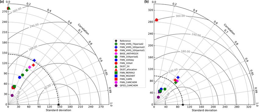
2842                                  B. Roozitalab et al.: Improving regional air quality predictions in the Indo-Gangetic Plain

Table 1. Details of WRF-Chem physical and chemical setup configuration.

                    Process                                Method
                    Domain                                 One domain (15 km horizontal resolution)
                    Land use                               MODIS 20 category
                    Time step                              60 s based on CFL stability criterion (Courant et al., 1928)
                    Vertical layers                        39 (top at 5 hPa)
                    Microphysics                           Morrison double-moment scheme (Morrison et al., 2005)
                    Longwave radiation                     RRTMG, called every 5 min
                    Shortwave radiation                    Goddard, called every 5 min
                    Planetary boundary layer               MYNN level 3 (Nakanishi and Niino, 2009)
                    Land surface                           Noah land surface model (Wang et al., 2018)
                    Gas-phase chemistry                    MOZART-4, called every 10 min
                    Photolysis scheme                      New TUV, called every 10 min
                    Aerosol scheme                         MOSAIC-4bin (no aqueous-phase chemistry), called every 10 min
                    Dust                                   GOCART (Ginoux et al., 2001)
                    Initial and boundary meteorology       NCEP FNL

Table 2. List of scenarios performed in this study.

   Simulation ID                            Initial or boundary chemical (gaseous   Biomass burning emission inventory      Dust
                                            and aerosol) conditions
   Reference scenario
   FINN_VIIRS_7Xperiod2 (base scenario)     CAM-chem     (gas)   and   MERRA-2      7 times higher (FINN and VIIRS) for 5   GOCART
                                            (aerosol)                               to 13 Nov
   Biomass burning emission sensitivities
   QFED_CAMCHEM                             CAM-chem (gas and aerosol)              QFED                                    GOCART
   FINN_CAMCHEM                             CAM-chem (gas and aerosol)              FINN                                    GOCART
   FINN_10Xall                              CAM-chem (gas) and MERRA-2              10-times-higher FINN                    GOCART
                                            (aerosol)
   FINN_10Xday                              CAM-chem (gas) and MERRA-2              10-times-higher FINN for 5 Nov          GOCART
                                            (aerosol)
   FINN_10Xperiod1                          CAM-chem (gas) and MERRA-2              10-times-higher FINN for 3 to 17 Nov    GOCART
                                            (aerosol)
   FINN_VIIRS_10Xperiod1                    CAM-chem (gas) and MERRA-2              10 times higher (FINN and VIIRS) for    GOCART
                                            (aerosol)                               3 to 17 Nov
   FINN_VIIRS_10Xperiod2                    CAM-chem (gas) and MERRA-2              10 times higher (FINN and VIIRS) for    GOCART
                                            (aerosol)                               5 to 13 Nov
   Boundary condition sensitivities
   FINN_MOZART                              MOZART (gas and aerosol)                FINN                                    GOCART
   FINN_CAMS                                CAMS (gas and aerosol)                  FINN                                    GOCART
   FINN_MERRA-2                             CAM-chem (gas) and MERRA-2              FINN                                    GOCART
                                            (aerosol)
   Dust emission sensitivities
   NO_DUST                                  CAM-chem     (gas)   and   MERRA-2      10-times-higher FINN                    Turned off
                                            (aerosol)
   DUST_5X                                  CAM-chem     (gas)   and   MERRA-2      10-times-higher FINN                    5-times-higher      GO-
                                            (aerosol)                                                                       CART emissions
   DUST_allocation                          CAM-chem     (gas)   and   MERRA-2      10-times-higher FINN                    GOCART, put 30 % of
                                            (aerosol)                                                                       bin 4 in bins 2 and 3
   Anthropogenic emission sensitivity
   BASE_ANTHRO2X                            Similar to base scenario (ID – FINN_ VIIRS_7Xperiod2) except anthropogenic aerosol emissions increased
                                            by a factor of 2

Atmos. Chem. Phys., 21, 2837–2860, 2021                                                            https://doi.org/10.5194/acp-21-2837-2021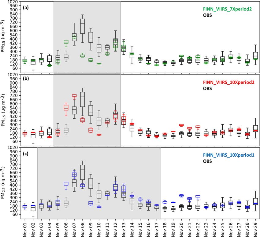
B. Roozitalab et al.: Improving regional air quality predictions in the Indo-Gangetic Plain                                 2843

confirmed the reliability of VIIRS-retrieved data (Fig. S5).      3     Results and discussions
MERRA-2 gridded data were also used to evaluate the model
performance. MERRA-2 reanalysis is based on the assimi-           3.1    Model performance
lation of many meteorological data and the assimilation of
AOD from multiple satellites (Gelaro et al., 2017). The on-       Our analysis comparing different simulations revealed that
ground continuous-monitoring station guidelines state that        the FINN_VIIRS_7Xperiod2 scenario had the best statisti-
instruments should sample at heights between 3–10 m. Ir-          cal performance of the configurations studied. This scenario
respective of this condition, some of the CPCB stations are       is called the base scenario, and we evaluate it in this sec-
placed on top of buildings with a restricted clean flow of air    tion. Performance of the base model in capturing the mete-
(personal inspections). While we observed little impact of        orological parameters was evaluated using MERRA-2 data
this situation on the concentrations in a well-mixed layer, a     for 10 m wind speed and direction, 2 m temperature, and the
meteorological parameter like wind speed data can show er-        surface water vapor mixing ratio. Figure 2a–d show these
ratic behavior. As a result, we used MERRA-2 meteorolog-          comparisons at the location of the US Embassy in Delhi
ical data to evaluate the WRF-Chem simulations using 10 m         (28.59◦ N, 77.19◦ E). The model was able to capture the
wind speed and direction, 2 m temperature, and surface water      general diurnal trend for all these variables and the sharp
vapor mixing ratio variables.                                     shift in wind direction between 13 and 17 November, af-
   We also compared MERRA-2 AOD (at 550 nm) and PM2.5             ter the extreme pollution episode. Negatively biased wind
predictions with WRF-Chem results to evaluate how the as-         speed with an ME of 1.1 m s−1 and RMSE of 1.28 m s−1
similation of AOD affected the predictions. The MERRA-2           shows the model generally underestimated wind speed, and
PM2.5 was based on the mass mixing ratios of black carbon,        it was most predominant between 17 and 25 November. Fig-
organic carbon, dust, sea salt, and sulfate. Since ammonium       ure 2c shows the model did not accurately capture night-
concentration is not available, it is common in the litera-       time 2 m temperature minima but captured the maximum val-
ture to assume that sulfate ion will be completely neutral-       ues with an overall overestimated ME of 3.52 ◦ C and RMSE
ized by ammonium and form ammonium sulfate, and there-            of 4.01 ◦ C. The wind speed satisfied the benchmark RMSE
fore a factor of 1.375 was assumed in calculating inorganic       value of 2.0 m s−1 , while temperature was higher than the tar-
aerosol concentrations (Buchard et al., 2016; He et al., 2019;    geted ME goal of 2.0 ◦ C (Emery et al., 2001). The representa-
Provençal et al., 2017). On the other hand, the literature sug-   tion error plays an important role in evaluating results due to
gests organic carbon concentration should be multiplied by        different horizontal resolutions in the model and MERRA-2
1.4 to compensate for other missing organic compounds to          dataset (∼ 0.15×0.15 vs. 0.625×0.5◦ ), specifically in urban
estimate the organic mass (Buchard et al., 2016; Chow et al.,     areas. For instance, the same statistics for a rural area in Ra-
2015; He et al., 2019; Provençal et al., 2017; Turpin and Lim,    jasthan (27.0◦ N, 73.0◦ E; not shown) have smaller biases and
2001). However, Turpin and Lim (2001) argued that this scal-      are compliant with benchmark values (RMSE of 0.99 m s−1
ing factor should be 2.6 for biomass burning particles; we        for wind speed and ME of 1.08 ◦ C for 2 m temperature). For
used 2.6 according to our studied time period and potential       the water vapor mixing ratio the model clearly captured the
black carbon sources:                                             daily variations, especially the increase after the pollution
                                                                  episode (13 November). However, it showed a very sharp
[PM] = [BC]+2.6·[OC]+1.375·[SO4 ]+[DUST]+[SS], (1)                day-to-night shift during the pollution episode days. The spa-
                                                                  tial performance of the model averaged over November dur-
where BC is black carbon, OC is organic carbon, SO4 is sul-       ing daytime hours (08:00 to 18:00 local time) is shown in
fate, DUST is dust, and SS is sea salt concentrations. As dust    Fig. 2e–j. The sharp gradient between the Himalayan and
and sea salt data are reported in multiple bins, different bins   IGP regions in the northeast, the gradient between land and
should be used for different particle diameters.                  sea in the southwest, and the slight gradient between differ-
   The metrics we used to assess the performance of the sim-      ent land types in the northwest of the domain for both 10 m
ulations were the root mean square error (RMSE), mean er-         wind speed and 2 m temperature were captured well. Over-
ror (ME), normalized mean bias (NMB), normalized mean             all, the model was able to capture the general daily variations
error (NME), and correlation coefficient (R) as defined in        and spatial trends when compared to MERRA-2 data.
the Supplement (Emery et al., 2017, 2001). Since low values          Figure 3 shows spatial distribution of the base scenario,
can have significant impacts on normalized values, which are      VIIRS data, and the bias for the 550 nm AOD, averaged over
used in mean normalized metrics, normalized mean values           all the days in November with 5 November as a day with
are better metrics and used in this study (Emery et al., 2017).   intensive fire emissions and 24 November as an illustrative
                                                                  day after the extreme pollution episode. The model showed
                                                                  high AODs over Delhi and Punjab, confirming satellite data.
                                                                  Moreover, AODs were high over the western IGP, close to
                                                                  major fires of Punjab, with a gradual gradient towards eastern
                                                                  and central India. Dust emission sources at the border of Pak-

https://doi.org/10.5194/acp-21-2837-2021                                           Atmos. Chem. Phys., 21, 2837–2860, 2021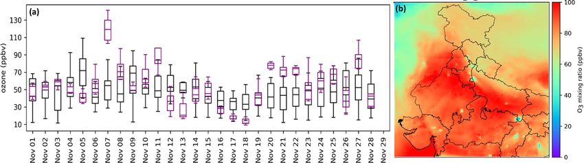
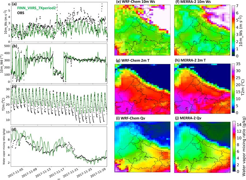
2844                            B. Roozitalab et al.: Improving regional air quality predictions in the Indo-Gangetic Plain

Figure 2. Temporospatial meteorological performance of base scenario simulation: time series of simulated (green line) and MERRA-
2 (black dots) hourly (a) 10 m wind speed, (b) 10 m wind direction, (c) 2 m temperature, and (d) surface water vapor at US Embassy
coordinates. (e, f) Averaged daytime (08:00–18:00 LT) 10 m wind speed maps of model (e) and MERRA-2 (f). (g, h) Averaged daytime
(08:00–18:00 LT) 2 m temperature maps of simulations (g) and MERRA-2 (h). (i, j) Averaged daytime (08:00–18:00 LT) surface water vapor
mixing ratio (g kg−1 ) maps of model (i) and MERRA-2 (j).

istan also led to high AODs although they did not affect Delhi       did not capture extremely high AODs over Punjab, although
as discussed in the Supplement. In general, the model under-         they showed AOD enhancements (Fig. S6).
estimates AOD over the IGP and overestimates it elsewhere.              Figure 4 shows time series of modeled, MERRA-2 prod-
WRF-Chem predicted the averaged AOD over the whole do-               uct, VIIRS-retrieved, and observed AOD at the AERONET
main for November 2017 to be 0.58 (±0.4), while VIIRS                stations (location shown in Fig. 1). AOD values at Kan-
data showed 0.43 (±0.26). AOD maps for 5 November show               pur, a station in the eastern IGP, were more than 1.0 be-
the model generally underestimated AOD values for the en-            fore the pollution episode, reached up to 2.0 during the
tire IGP region, except for Punjab. Moreover, the model un-          episode days, and decreased to values of between 0.5 and
derestimated aerosol loadings over central India. Other stud-        1 for the rest of the days. The model captured the general
ies have reported biased-low AOD and corresponding PM2.5             trend although missed high AODs between 9 and 13 Novem-
concentrations over other polluted regions (He et al., 2019;         ber, while MERRA-2 successfully captured the AOD trend
Song et al., 2018). On the other hand, 24 November repre-            through the whole month, including days with enhanced
sented a day with no significant fire emissions. The model           AOD values. This shows that AOD assimilation in MERRA-
did a good job capturing AOD values in the central parts             2 significantly improves AOD predictions. At Jaipur, located
of India and around Delhi. However, the model missed high            in the southern IGP, the model overestimated AOD for the
AOD values in the eastern IGP. MERRA-2 data also did not             first 5 d of November. During the pollution episode days,
show high AODs over the western border with Pakistan and             the model is biased high compared to MERRA-2 and VI-

Atmos. Chem. Phys., 21, 2837–2860, 2021                                                https://doi.org/10.5194/acp-21-2837-2021
B. Roozitalab et al.: Improving regional air quality predictions in the Indo-Gangetic Plain                                2845

IRS retrievals. AERONET data showed low AOD values              concentrations for the next 3 d. Then, the model captured the
before the pollution episode but did not report values dur-     second enhancement. Although wind direction showed good
ing the pollution episode. This suggests, as one possibil-      agreement with the MERRA-2 dataset and wind speed was
ity, that PM concentrations were too high during this period    biased low and even more favorable for stagnant conditions,
for the instrument to retrieve data. After the pollution pe-    modeled PM2.5 concentrations had a large negative bias for
riod, AOD values were lower than 0.5, showing relatively        the period between 8 and 10 November. This suggests ei-
low PM concentrations. In general, MERRA-2 showed better        ther low local anthropogenic emissions within Delhi or some
performance in terms of NMB (Kanpur −1.3 % and Jaipur           missing pollution sources upwind of Delhi that were not in-
−20.1 %) compared with our model (Kanpur: −27.4 % and           cluded in the emission estimates led to underestimation.
Jaipur: +29.9 %). Comparing averaged AOD with VIIRS re-            Dekker et al. (2019) studied CO concentrations during
trievals for the BASE_ANTHRO2X scenario showed lower            November 2017 using satellite observations, and they re-
bias over the IGP (Fig. S7). These results show the need for    ported low emissions as one of the reasons for large nega-
improved estimates of biomass burning as well as anthro-        tive concentration biases, although they proposed unfavor-
pogenic emissions. We also looked at the Ångström expo-         able meteorological conditions as the main reason for high
nent (AE) at Jaipur and Kanpur to understand if the model       CO concentrations in Delhi, between 11 and 14 Novem-
captured the mode of the particles (Fig. S8). Over Jaipur the   ber. Moreover, Cusworth et al. (2018) reported that MODIS-
model is biased high compared to AERONET data (NMB              based biomass burning emission inventories miss many small
30 %) and shows more finer aerosols in the model. After         fires over India. Beig et al. (2019) concluded that long-range-
20 November, both AERONET and VIIRS retrievals sug-             transported dust coming from the Middle East was a major
gest the dominance of coarser aerosols, while the AE for the    source for this extreme pollution episode. Figure 5a shows
model does not follow the same trend. However, the modeled      that MERRA-2 did not capture high surface PM2.5 concen-
PM2.5 / PM10 ratio shows more coarse aerosols compared to       trations after 8 November. Navinya et al. (2020) reported that
the rest of the month (Fig. S9). Over Kanpur, the model AE      MERRA-2 underestimates PM2.5 over India, especially dur-
is biased high (NMB: 50.8 %). On the other hand, the model      ing the post-monsoon season. More discussions on the ex-
shows closer AE values to VIIRS retrievals. For example,        treme pollution episode are provided in the following sec-
both the model and VIIRS retrieval show similar reduction       tion.
in the AE on 8 and 9 November. Kumar et al. (2014b) also           Starting on 13 November, the modeled concentrations
reported slight AE overestimation in WRF-Chem during a          went down as winds shifted to easterlies and wind speed in-
pre-monsoon dust storm at Kanpur and Jaipur. Furthermore,       creased. Beig et al. (2019) found PM2.5 concentrations af-
the model and AERONET have a variational trend while            ter the pollution episode were lower compared with simi-
MERRA-2 is smooth during the whole month at both Jaipur         lar periods in previous years. Thereafter, the concentrations
and Kanpur.                                                     went back to values for Delhi before the episode. The model
   Figure 5a shows time series plots of base scenario and ob-   did a fairly good job of capturing the trend during non-
served PM2.5 concentration at the US Embassy station. Ob-       episode days (Table S4). Increasing anthropogenic emissions
served values were high throughout the month on the or-         (ID – BASE_ANTHRO2X) on simulation results overesti-
der of 200 µg m−3 with diurnal variations due to changes        mated PM2.5 concentrations in the US Embassy location dur-
in the mixing heights. The extreme pollution episode be-        ing non-episode days (Fig. S7).
gan on 7 November, when PM2.5 concentrations increased             Figure 5b and c show the averaged PM2.5 maps for all
to more than 800 µg m−3 . On 8 November, the values in-         the hours over the studied region in the base simulation and
creased even more to about 1000 µg m−3 . PM2.5 concentra-       MERRA-2 dataset. The model was able to capture higher
tions started decreasing on 9 November and continued de-        concentrations over northwestern India and the border with
creasing through 10 November. However, values increased         Pakistan where agricultural fire and dust emissions play the
again and were high between 11 and 13 November. After-          most important role for extreme pollution episodes over IGP.
wards, they returned to ∼ 200 µg m−3 for the rest of the        However, the model showed higher values than MERRA-2
month. The model accurately captured the magnitude and di-      over southern Punjab, a region with high biomass burning
urnal cycle for PM2.5 for non-episodic days. Moreover, the      emissions (Kulkarni et al., 2020). Since MERRA-2 assimi-
model was able to see the sharp increase in concentration       lates satellite AOD data as its major aerosol forcing, it will
in the beginning of the episode starting from 7 November        not be able to capture high concentrations if satellite retrieval
with reported PM2.5 concentrations of ∼ 650 µg m−3 . This       algorithms miss corresponding high AODs.
sharp increase was captured after incorporating VIIRS data         Figure 5b and c also show that the model was biased high
into FINN emissions accompanied by scaling the emissions        over central India and biased low over the eastern IGP. These
by a factor of 7. In fact, increased emissions from fires in    results indicate improving emissions in the eastern IGP can
agricultural fields in the northwest on previous days and fa-   significantly improve the simulation results. Conibear et
vorable northwesterly winds, as shown in Fig. 2, explain this   al. (2018a) also reported limited success of models to capture
concentration hike. However, the model underestimated the       the spatial variability in PM2.5 over India in 2016, specifi-

https://doi.org/10.5194/acp-21-2837-2021                                         Atmos. Chem. Phys., 21, 2837–2860, 2021
2846                            B. Roozitalab et al.: Improving regional air quality predictions in the Indo-Gangetic Plain

cally during winter. Table 3 provides statistics for 24 h aver-    3.2   Extreme-pollution-episode analysis
aged PM2.5 concentrations for the base scenario simulation
for Delhi and its western states. Statistics for Delhi show an     Figure 6a shows the box-and-whisker plots for daily PM2.5
NMB of −16.6 %, which passes the “criteria” benchmark of           concentration for the base scenario and all of the CPCB sta-
30 %, while an NME of 27.6 % shows better performance and          tions in Delhi. Over all CPCB stations in Delhi, 24 h aver-
complies with the benchmark “goal” of 35 % for the whole           aged measured values for PM2.5 ranged between 133 and
month (Emery et al., 2017). A correlation coefficient of 0.48      664 µg m−3 , which is about 2 and 11 times higher, respec-
is also higher than the benchmark criterion of 0.4. Statistics     tively, than the India 24 h standard value of 60 µg m−3 . The
significantly improve after excluding the 4 extremely pol-         model showed overall good performance for daily PM2.5
luted days between 7 and 10 November and all are within            concentrations for days without extreme pollution (Table S4;
benchmark goals (Table S4). Kumar et al. (2020) assimilated        NMB of −2.44 and R of 0.7) and followed the observed
MODIS AOD into WRF-Chem in order to improve the air                trend in the extreme pollution episode (Fig. 6), which sug-
quality forecasts over Delhi. In their study, the mean bias        gests the overall meteorology and transport patterns were
for first-day forecast of PM2.5 concentration decreased from       captured by the simulations. However, the model started the
−98.7 to −13.7 µg m−3 . They also showed that the RMSE             episode on 6 November and significantly overestimated the
decreased from 167.4 to 117.3 µg m−3 . Our results from the        concentrations. The model captured the median for 7 Novem-
base scenario (mean bias of −42.38 µg m−3 and RMSE of              ber very well, although measured values span a wider range.
118.47 µg m−3 ) show comparable results to the data assimi-        The model missed the high concentrations on 8 Novem-
lation technique, although both models are still biased low.       ber, which led to underestimations on 9 and 10 November,
   Statistics for the state of Haryana (4 stations) show good      as well, regardless of capturing the decreasing trend. How-
performance (NMB of −7.5 % and correlation coefficient             ever, the model was able to simulate the second wave of the
of 0.4). The model was biased high for Rajasthan (10 sta-          episode starting on 11 November and accurately captured
tions, NMB 15.5 %) and Punjab (3 stations, NMB 17 %).              the median and range of PM2.5 concentrations on 12 and
The model slightly overestimated PM2.5 concentrations dur-         13 November. It is important to point out that the underes-
ing the episode days in Rajasthan but captured the concen-         timation of PM on 9 and 10 November persisted for all of the
trations during the rest of the month (Fig. S10). In Punjab,       sensitivity cases performed. This suggests the transport in the
measured data did not report PM2.5 enhancement during the          model during these days missed highly polluted source re-
extreme episode, while the model showed very high concen-          gions or significant emission sources for these days were not
trations after scaling fire emissions by a factor of 7. However,   included in the inventories or both.
VIIRS satellite images (e.g., Fig. 9d) clearly show massive           Back trajectories can be used to provide insights into mod-
agricultural fires in this state during November, and its sig-     eled concentrations during the extreme pollution episode.
nals were expected in the measured data. The overall scatter-      Back trajectories were calculated for releasing 10 000 air
plots including the averaged values for each state show good       parcels at 100 m above ground level and over eastern Delhi
spatial performance of the base scenario (Fig. S11).               using the FLEXible PARTicle dispersion model (FLEX-
   Although different meteorological parameters can be re-         PART) with inputs from WRF-Chem output (Brioude et al.,
sponsible for the biases, accuracy of anthropogenic emis-          2013). Figure 7 shows 72 h mean back trajectory maps for
sions is important. For example, recent local anthropogenic        6, 7, 8, 9, and 10 November. The releasing times are 00:00
emission inventories developed for Delhi have higher par-          (red line; denoted by the suffix _00 in the text below) and
ticle emissions than in the regional inventory used in this        12:00 (blue line; denoted by the suffix _12 in the text be-
study, which impacts modeled PM2.5 concentrations for              low) UTC on each day. Also plotted are the fire (gray line)
typical days (Kulkarni et al., 2020). We conducted the             and anthropogenic (black line) emissions along the trajec-
BASE_ANTHRO2X scenario to investigate the effect of                tory. The model started to build up PM2.5 concentrations on
uncertainties in the anthropogenic emissions. This sce-            6 November and was biased high (Fig. 6a). Back trajecto-
nario increased PM2.5 concentrations in Delhi to up to ∼           ries for 6 November_00 show PM2.5 concentrations were
150 µg m−3 , which led to overestimation (in contrast to un-       majorly due to anthropogenic emissions (Fig. 7a). However,
derestimation in the base scenario) on many of the non-            6 November_12 trajectories in Fig. 7c show a spike in fire
episode days (Fig. S7). Although this scenario did not help        emissions at previous hours (backward hours 5 and 30),
in capturing the high concentrations during the episode, it        which immediately led to high PM2.5 concentrations. More-
confirms the need for better anthropogenic emissions. On the       over, trajectory paths for this day reveal that emissions be-
other hand, it reduced the bias over the IGP (Fig. S7). These      longed to fires east of Delhi. Figure 9 shows that the fires
results point out the need for best estimates of both anthro-      east of Delhi in the base scenario are due to incorporating
pogenic and biomass emissions. Maps also show that aver-           VIIRS data into the fire emissions. Therefore, high-biased
aged PM2.5 concentrations over most of India were higher           PM2.5 concentration may be related to the scaling factor ap-
than the air quality standard.                                     plied to eastern Delhi fires. On 7 November, the model per-
                                                                   fectly captured the PM2.5 median (Fig. 6a). Back trajecto-

Atmos. Chem. Phys., 21, 2837–2860, 2021                                             https://doi.org/10.5194/acp-21-2837-2021
B. Roozitalab et al.: Improving regional air quality predictions in the Indo-Gangetic Plain 2847 Figure 3. Spatial distributions of AOD at 550 nm averaged over the whole of November (a–c), 5 November (d–f), and 24 November (g–i). WRF-Chem maps represent base scenario results. Differences between model and VIIRS are also shown. ries for 7 November_00 (Fig. 7d, e) show the beginning of ber_00 crossed through central parts of Punjab. Moreover, lo- a shift in wind direction and PM2.5 concentration was ex- cal anthropogenic emission sources affected 8 November_00 clusively due to fire emissions on 5 November (backward trajectories. The model underestimated PM2.5 concentrations hour 40). Compared to 7 November_00, fire emission foot- on 8 November, which can be partly related to errors in trans- prints for 7 November_12 trajectories are smaller, while local port as the trajectories for 8 November_12 crossed eastern anthropogenic emissions are higher (Fig. 7f). Back trajecto- parts of Punjab. However, other physical processes or lower ries for 8 November show the northern parts’ contribution anthropogenic emissions can also be responsible for low- for both releasing times, although trajectories for 8 Novem- biased concentrations. Delhi’s air quality for 9 November_00 https://doi.org/10.5194/acp-21-2837-2021 Atmos. Chem. Phys., 21, 2837–2860, 2021
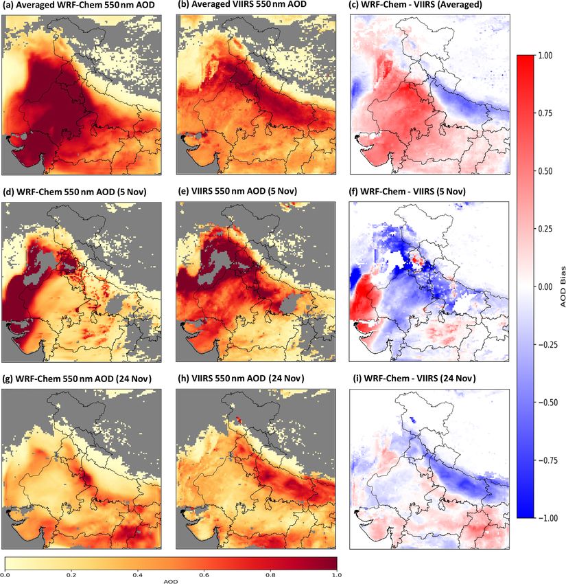
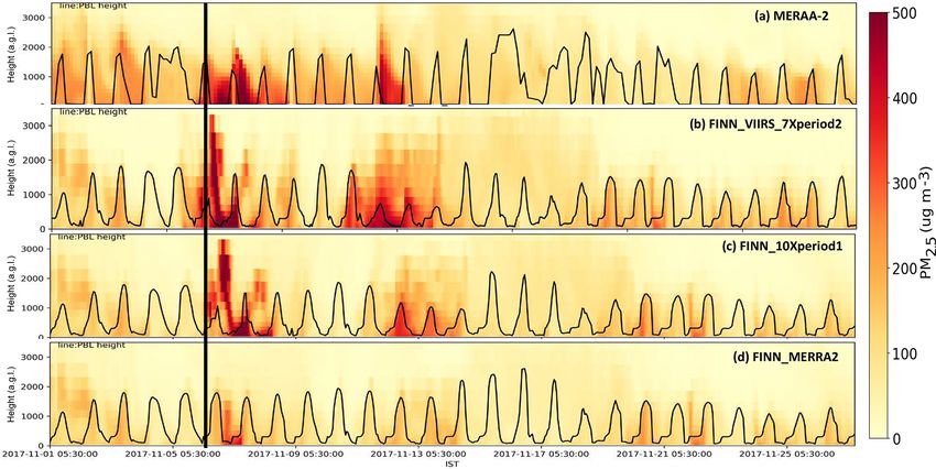
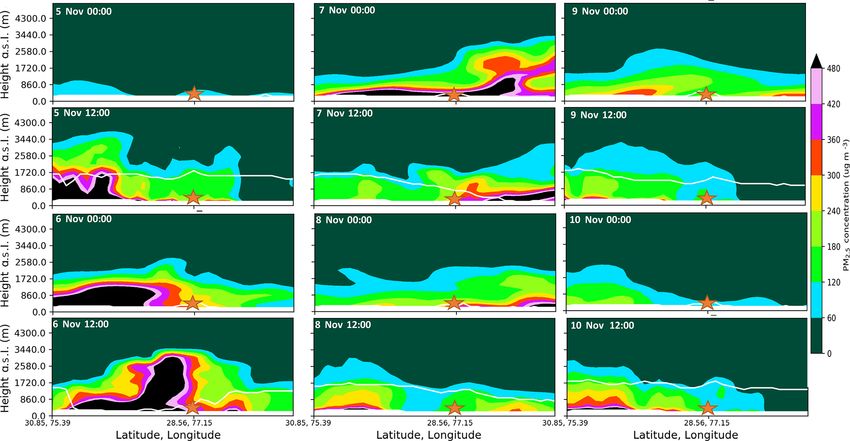
2848                             B. Roozitalab et al.: Improving regional air quality predictions in the Indo-Gangetic Plain

Figure 4. Time series of modeled (green line), VIIRS-retrieved (blue triangles), MERRA-2 (red line), and AERONET (black dots) AOD at
550 nm during November 2017 at (a) Jaipur and (b) Kanpur.

Figure 5. Temporospatial air quality performance of base scenario simulation: (a) time series of simulated (green line), MERRA-2 (red line),
and ground measurement (black dots) hourly PM2.5 concentration at US Embassy coordinates. (b, c) Hourly averaged PM2.5 concentration
maps of model regridded to MERRA-2 resolution (b) and MERRA-2 (c).

was still being affected by northern parts, while trajectories          the smoke upwind of Delhi blew over Delhi and led to ex-
for 9 November_12 shifted towards the east. Since trajecto-             tremely high concentrations. Although the model captured
ries for 9 November do not show any fire or anthropogenic               the median on 7 November, it missed the maximum extent
emission pulse, the model missed either the dynamics of that            of observed values. Cross sections on 8, 9, and 10 November
day or emission sources. Trajectories for 10 November show              show Punjab’s residual smoke in the boundary layer, while
eastern flow, again, and no fire emission contribution.                 we saw the model underestimated PM2.5 concentrations on
   To further understand the regional-scale transport of the            these days. Measured PM2.5 concentrations over Delhi show
smoke plumes, we plotted a cross section of PM2.5 over the              a decreasing trend between 8 and 10 November (Fig. 6). Ver-
path from Punjab through Delhi (Fig. 8, path line shown                 tical profiles for the base scenario also show the model cap-
in Fig. 1). PM2.5 concentrations showed typical values for              tured a high biomass burning emission period on 6 November
5 November_00 although they still exceeded the standard                 (Fig. 12). However, it also showed high amounts of smoke
limits. For 5 November_12, concentrations significantly in-             above the planetary boundary layer (PBL). Cross sections
creased over Punjab area because of fires, and the winds                for 11 to 14 November can be found in the Supplement
brought them on a path towards Delhi. The Punjab’s smoke                (Fig. S12). These results suggest that plume rise in the model
had not yet completely crossed Delhi on 6 November as back              released the emissions too high or the model did not mix the
trajectories for 00:00 and 12:00 UTC hours also showed the              smoke down fast enough. Using an ECMWF map, Vijayaku-
effects of anthropogenic emissions and fires in eastern Delhi.          mar et al. (2016) showed agricultural fires can transport parti-
On the other hand, a significant amount of smoke was above              cles via the upper troposphere and subside over Delhi. Social
the boundary layer as shown in the 6 November_12 panel.                 reasons can also be important as the first reaction of people
Due to shifting winds on 7 November (as shown in Fig. 2),

Atmos. Chem. Phys., 21, 2837–2860, 2021                                                    https://doi.org/10.5194/acp-21-2837-2021
B. Roozitalab et al.: Improving regional air quality predictions in the Indo-Gangetic Plain 2849
Table 3. Mean (± standard deviation), normalized mean bias (NMB), normalized mean error (NME), and Pearson’s correlation co-
efficient (R) averaged for all CPCB stations in different states during November 2017. Model values are for the base scenario
(FINN_VIIRS_7Xpeiod2). Mean values are for hourly data, while NMB, NME, and R relate 24 h averaged values.
State Hourly obs. mean (± SD) Hourly model mean (± SD) 24 h NMB 24 h NME 24 h R
(µg m−3 ) (µg m−3 ) (%) (%) (%)
Delhi 255.5 (±146.6) 213.9 (±113.9) −16.6 27.6 0.48
Haryana 177.7 (±77.6) 165.8 (±89.9) −7.5 29.5 0.40
Punjab 139.9 (±54.7) 166.7 (±198.3) 17 55.5 0.24
Rajasthan 123.4 (±62.7) 147.7 (±62.7) 15.5 34.4 0.22
during hazy days is to drive to work which directly (exhaust air quality. Our results confirm that FINN provides better
emissions) and indirectly (road dust) worsens air pollution. biomass burning emissions for India for this period and shed
light on the importance of choosing a proper biomass burning
3.3 Sensitivity to changes in biomass burning emission emission inventory for a specific domain.
inventories However, the signals from the simulation using the FINN
biomass burning emission inventory were not high enough as
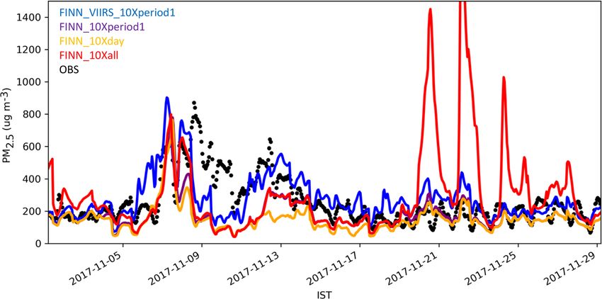
Biomass burning emissions used in the base scenario in or- it recorded a maximum concentration of 400 µg m−3 while
der to capture the extreme pollution episode were tuned after the corresponding measured value was 680 µg m−3 . Since
exploring how these inventories influenced PM2.5 concen- observation data are sporadic over India and there were not
trations (Table S3). First, we looked at two different emis- many ground measurement stations available, sophisticated
sion inventories based on different methodologies and hori- techniques such as inversion modeling were not feasible
zontal resolutions, specifically, FINNv1.5 and QFEDv2.5r1. (Saide et al., 2015). As a result, manual tuning of the emis-
Both inventories rely on MODIS data; FINN is based on ac- sion data was performed. The first attempt was to understand
tive fire points and estimates of burned area, whereas QFED if FINN was required to be increased for the whole month; a
uses an FRP approach (Pan et al., 2020). Figure 9 shows the 15 d period around the episode; or just on 5 November, which
grid cells with biomass burning emissions based on QFED had many fire points in Punjab (Fig. 9). Figure 10 shows
(panel a), FINN (panel b), and FINN_VIIRS composition PM2.5 time series averaged over all CPCB stations based on
(panel c), used in the base scenario, accompanied by active these scenarios. Increasing FINN emissions for the whole
fire points seen by VIIRS (panel d) based on the Fire Infor- month (ID – FINN_10Xall) led to an overestimation in the
mation for Resource Management System (FIRMS) product first 5 d of November, but it significantly helped in capturing
for 5 November. It shows FINN captured more fire points in high peaks on 7 and 8 November. Moreover, it increased the
the domain although missed some in the eastern IGP and cen- concentrations on 12 and 13 November regardless of missing
tral India while QFED missed almost all of the fire points in the peaks. However, it did not show any improvements be-
Punjab on that specific day. As a result, the QFED simulation tween 9 and 12 November, which suggests that the included
did not show any major signal for PM2.5 concentration on fires did not influence Delhi’s air quality during this period.
7 November, whereas the experiment using the FINN inven- On the other hand, increasing FINN emission data by a factor
tory (ID – FINN_CAMCHEM) followed the measured start of 10 for all days led to very high PM2.5 concentrations on
of the episode period, regardless of its low-biased PM2.5 con- later days (20–27 November). This showed that FINN data
centrations (Fig. S13). In general, results using the QFED in- were not systematically biased low. In other words, these
ventory had worse statistics (Fig. 11 and Table S3), which is results suggest that the FINN algorithm underestimated the
mostly due to the inability of the inventory to capture the fire magnitude of only some fires emission amounts. Some stud-
points over the domain, and it can be attributed to both the ies have shown that thick fires can be identified as clouds
technique and the resolution as QFED data have a ∼ 10 km in retrieval algorithms (Dekker et al., 2019; Huijnen et al.,
resolution, whereas FINN data have a ∼ 1 km resolution. 2016). As another experiment, we increased FINN emissions
Pan et al. (2020) found high uncertainty between different only on 5 November since that day had original high val-
biomass burning emission inventories over Southeast Asia. ues in the inventory (ID – FINN_10Xday). This experiment
They showed FINN is, in general, a better dataset for trop- resulted in better PM2.5 concentrations in the last third of
ical regions as its 2 d continuous fire emissions compensate November. However, it captured only the high concentra-
for the lack of daily MODIS coverage used in QFED (Pan tions of 7 November and missed the peak of 8 November
et al., 2020; Wiedinmyer et al., 2011). Dekker et al. (2019) as well as underestimated concentrations on some other days
increased the GFAS biomass burning emission inventory by including 13 November. Finally, we multiplied the fire emis-
a factor of 5, did not see any improvement to CO simulation, sions by 10 for a 15 d period between 3 and 17 November
and reported about a 2 % contribution from fires to Delhi’s
https://doi.org/10.5194/acp-21-2837-2021 Atmos. Chem. Phys., 21, 2837–2860, 2021You can also read