Statistical modelling of co-seismic knickpoint formation and river response to fault slip
←
→
Page content transcription
If your browser does not render page correctly, please read the page content below
Earth Surf. Dynam., 7, 681–706, 2019
https://doi.org/10.5194/esurf-7-681-2019
© Author(s) 2019. This work is distributed under
the Creative Commons Attribution 4.0 License.

                 Statistical modelling of co-seismic knickpoint
                   formation and river response to fault slip
                      Philippe Steer1 , Thomas Croissant1,a , Edwin Baynes1,b , and Dimitri Lague1
                      1 Univ
                           Rennes, CNRS, Géosciences Rennes – UMR 6118, 35000 Rennes, France
                           a nowat: Department of Geography, Durham University, Durham, UK
      b now at: Department of Civil and Environmental Engineering, University of Auckland, Auckland, New Zealand

                               Correspondence: Philippe Steer (philippe.steer@univ-rennes1.fr)

                                  Received: 5 February 2019 – Discussion started: 14 February 2019
                               Revised: 10 June 2019 – Accepted: 3 July 2019 – Published: 24 July 2019

      Abstract. Most landscape evolution models adopt the paradigm of constant and uniform uplift. It results that the
      role of fault activity and earthquakes on landscape building is understood under simplistic boundary conditions.
      Here, we develop a numerical model to investigate river profile development subjected to fault displacement by
      earthquakes and erosion. The model generates earthquakes, including mainshocks and aftershocks, that respect
      the classical scaling laws observed for earthquakes. The distribution of seismic and aseismic slip can be parti-
      tioned following a spatial distribution of mainshocks along the fault plane. Slope patches, such as knickpoints,
      induced by fault slip are then migrated at a constant rate upstream a river crossing the fault. A major result
      is that this new model predicts a uniform distribution of earthquake magnitude rupturing a river that crosses a
      fault trace and in turn a negative exponential distribution of knickpoint height for a fully coupled fault, i.e. with
      only co-seismic slip. Increasing aseismic slip at shallow depths, and decreasing shallow seismicity, censors the
      magnitude range of earthquakes cutting the river towards large magnitudes and leads to less frequent but higher-
      amplitude knickpoints, on average. Inter-knickpoint distance or time between successive knickpoints follows an
      exponential decay law.
         Using classical rates for fault slip (15 mm year−1 ) and knickpoint retreat (0.1 m year−1 ) leads to high spatial
      densities of knickpoints. We find that knickpoint detectability, relatively to the resolution of topographic data,
      decreases with river slope that is equal to the ratio between fault slip rate and knickpoint retreat rate. Vertical
      detectability is only defined by the precision of the topographic data that sets the lower magnitude leading to
      a discernible offset. Considering a retreat rate with a dependency on knickpoint height leads to the merging
      of small knickpoints into larger ones and larger than the maximum offset produced by individual earthquakes.
      Moreover, considering simple scenarios of fault burial by intermittent sediment cover, driven by climatic changes
      or linked to earthquake occurrence, leads to knickpoint distributions and river profiles markedly different from
      the case with no sediment cover. This highlights the potential role of sediments in modulating and potentially
      altering the expression of tectonic activity in river profiles and surface topography. The correlation between the
      topographic profiles of successive parallel rivers cutting the fault remains positive for distance along the fault
      of less than half the maximum earthquake rupture length. This suggests that river topography can be used for
      paleo-seismological analysis and to assess fault slip partitioning between aseismic and seismic slip. Lastly, the
      developed model can be coupled to more sophisticated landscape evolution models to investigate the role of
      earthquakes on landscape dynamics.

Published by Copernicus Publications on behalf of the European Geosciences Union.
682                                                      P. Steer et al.: Statistical modelling of co-seismic knickpoint formation

1   Introduction                                                     ond by the already-well-understood role of isostasy and vis-
                                                                     cous deformation on topography (e.g. Watts, 2001; Braun,
The interactions among tectonics, climate and surface pro-           2010). In active mountain belts, displacement along frontal
cesses govern the evolution of the Earth’s topography (e.g.          thrust faults can lead to the development of co-seismic wa-
Willet, 1999; Whipple, 2009). Among the potential link               terfalls, knickpoints and knickzones than can reach several
and feedbacks between tectonics and surface processes, the           metres in elevation (e.g. Boulton and Whittaker, 2009; Yan-
building of topographic slopes by tectonic deformation is            ites et al., 2010; Cook et al., 2013). These differential to-
critical. Erosion rates and most geomorphological processes          pographies, associated with high slopes, are referred to as
are strongly sensitive to local slope, including river incision      slope patches in the following work. These slope patches
(e.g. Whipple and Tucker, 1999), glacial carving (e.g. Her-          have long been recognized as potential markers of the dy-
man and Braun, 2008), soil creep (e.g. McKean et al., 1993)          namic response of rivers (e.g. Gilbert, 1896) to transient con-
and hillslope mass wasting (e.g. Keefer, 1994). The depen-           ditions, not limited to changes in tectonic activity, and in-
dency on slope can be linear or non-linear, mainly due to            cluding base level fall and lithological contrasts, among oth-
threshold effects or to a power-law behaviour. For instance,         ers. Yet, in active tectonic areas, knickpoints are frequently
a theoretical model combined with a data compilation sug-            associated with fault activity and transience in uplift rate (e.g.
gests that river incision rate is linearly dependent on slope        van der Beek et al., 2001; Quigley et al., 2006; Dorsey and
at knickpoints and more than linearly dependent on slope             Roering, 2006; Yildirim et al., 2011). These slope patches
for more gentle stream profiles (Lague, 2014). This is piv-          generated by frontal thrusts along a river migrate upstream
otal, as temporal variations in tectonic displacement and in         by erosion and are expected to set the erosion rate of the
slope building cannot be averaged out when considering river         entire landscape (Rosenbloom and Anderson, 1994; Royden
profile evolution using an erosion law with a non-linear de-         and Perron, 2013; Yanites et al., 2010; Cook et al., 2013).
pendency on slope. In addition to slope, the height of knick-           Fault slip and surface rupture classically occur by seis-
points (i.e. with a slope above average local slope) and wa-         mic slip during earthquakes. However, associating individual
terfalls (i.e. with a slope close to infinity) appears as a funda-   earthquakes with knickpoints or associating series of knick-
mental ingredient of their survival, retreat rate and river in-      points with series of earthquakes remains challenging from
cision (Hayakawa and Matsukura, 2003; Baynes et al., 2015;           field data. We therefore use in this paper a statistical model
Scheingross and Lamb, 2017). Similar issues arise for hill-          of earthquakes to simulate the expected slope and height dis-
slope dynamics impacted by fault scarp development (Ar-              tributions of the slope patches generated by earthquakes (i.e.
rowsmith et al., 1996) and possibly for faults in glaciated          fault seismic slip) and fault aseismic slip at the intersec-
landscapes. Despite this, most landscape evolution models of         tion between a thrust fault and a river. This model uses the
topographic growth consider slope building as a continuous           branching aftershock sequence (BASS) model (Turcotte et
process resulting from a constant (or smoothly varying) up-          al., 2007) to simulate temporal and spatial series of earth-
lift rate (e.g. Braun and Willett, 2013; Thieulot et al., 2014;      quakes based on the main statistical and scaling laws of
Campforts et al., 2017). There is therefore a clear need to de-      earthquakes. The rupture extent and displacement of earth-
fine how tectonic deformation builds topographic slopes in           quakes are inferred using classical scaling laws (Leonard,
numerical models.                                                    2010). We focus on the response of rivers and analyse the re-
   The expression of tectonic deformation on topographic             sulting knickpoint height distribution and their migration dis-
slope is diverse, and its spatial and temporal scales range          tance along a single river in near-fault conditions. We also in-
from metres to continents and from instantaneous to geo-             fer the correlation between the topography of successive par-
logical times, respectively. Tectonic deformation can (1) in-        allel rivers distributed along the strike of a single fault. The
stantaneously generate steep-to-infinite slopes when earth-          obtained results are then discussed with regards to the poten-
quakes rupture the Earth’s surface (e.g. Wells and Copper-           tial of knickpoints and waterfalls to offer paleo-seismological
smith, 1994); (2) induce progressive slope building at the           constraints and to the necessity of considering time-variable
orogen scale and over a seismic cycle by aseismic deforma-           uplift accounting for earthquake sequences in landscape evo-
tion (i.e. deformation not associated with earthquakes) and          lution models. It is important to stress that this study does
interseismic deformation (i.e. deformation occurring in be-          not aim to investigate specific geomorphological settings but
tween large-magnitude earthquakes) (e.g. Cattin and Avouac,          to give general theoretical and modelling arguments to the
2000) or by the deformation associated with earthquakes              interpretation of river profiles upstream of active faults.
with no surface rupture; and (3) lead to longer-term topo-
graphic tilting at the orogen-to-continental scale by isostatic
readjustment (e.g. Watts, 2001) or viscous mantle flow (e.g.
Braun, 2010). In this paper, we focus on the building of to-
pographic slopes by fault slip at the intersection between a
fault trace and a river. This is motivated first by the fact that
the greatest slopes are expected to occur by faulting and sec-

Earth Surf. Dynam., 7, 681–706, 2019                                                      www.earth-surf-dynam.net/7/681/2019/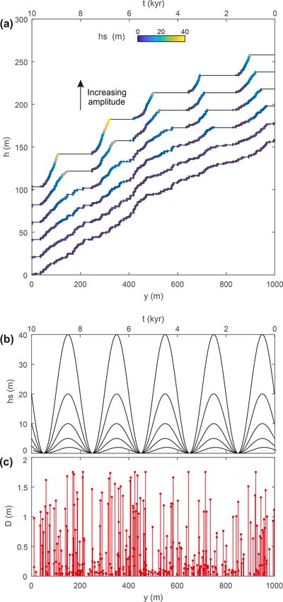
P. Steer et al.: Statistical modelling of co-seismic knickpoint formation                                                   683

2     State of the art: linking fault slip to knickpoint           in turn to aseismic slip (Scholz, 1998). This probably cen-
      formation and migration                                      sors the magnitude range of earthquakes rupturing the sur-
                                                                   face towards large magnitudes associated with rupture extent
2.1    From fault slip and earthquakes to surface ruptures         greater than this minimum seismogenic depth.
       and knickpoints
In near-fault conditions, too few data characterizing fault        2.2   Knickpoint formation
rupture geometry at one location (e.g. along a river) exist to
                                                                   The transformation of surface ruptures into knickpoints re-
assess the distribution of the slope and height of surface rup-
                                                                   mains a relatively enigmatic issue. Linking knickpoints to in-
tures resulting from earthquakes by local fault activity (e.g.
                                                                   dividual earthquakes is challenging, although some recently
Ewiak et al., 2015; Wei et al., 2015; Sun et al., 2016). Re-
                                                                   formed knickpoints have been clearly identified as the result
gional or global compilation of fault rupture by earthquakes
                                                                   of the surface rupture of a single large earthquake (e.g. Yan-
(e.g. Wells and Coppersmith, 1994; Leonard, 2010; Boncio
                                                                   ites et al., 2010; Cook et al., 2013). The transformation of
et al., 2018) offers another approach, that yet suffers from
                                                                   individual surface ruptures into individual co-seismic knick-
inescapable statistical biases mainly due to the use of faults
                                                                   points is not necessarily a bijective function and is more
with different slip rates, dimensions, seismogenic properties
                                                                   likely to be a surjective function. In other words, a knick-
and records of paleo-earthquakes. In addition, small earth-
                                                                   point can be made of several surface ruptures. Indeed, if the
quakes associated with small rupture extents and co-seismic
                                                                   time interval between two (or more) successive ruptures at
displacement are less likely to be identified in the field. For
                                                                   the same location is less than a characteristic migration time
instance, using seismological scaling laws (Leonard, 2010),
                                                                   required to segregate their topographic expressions, then the
an earthquake of magnitude 3 on a thrust fault has a rupture
                                                                   formed knickpoint will result from this succession of surface
length of 188 m and an average displacement of 1.2 cm. This
                                                                   ruptures and earthquakes. An end-member setting favouring
displacement is clearly below the precision of current dig-
                                                                   this behaviour is the case of fault scarps developing on hill-
ital elevation models or in any case hidden by the inherent
                                                                   slopes, whose degradation is generally assumed to follow a
topographic roughness.
                                                                   diffusion law (e.g. Nash, 1980; Avouac, 1993; Arrowsmith
   Statistical or theoretical inferences offer another means
                                                                   et al., 1996; Roering et al., 1999; Tucker and Bradley, 2010).
to associate fault activity and earthquakes with surface rup-
                                                                   Moreover, in the downstream part of rivers, fault scarps can
tures and knickpoints. Earthquakes tend to universally follow
                                                                   remain buried under a sediment cover due to, for instance, the
the Gutenberg–Richter frequency–magnitude distribution in
                                                                   development of an alluvial fan (Finnegan and Balco, 2013;
Eq. (1):
                                                                   Malatesta and Lamb, 2018). Development of the fault scarp
log10 (N (≥ Mw )) = a − bMw ,                               (1)    height by successive ruptures or the thinning of the alluvial
                                                                   cover can then expose the scarp, in turn potentially forming
where Mw is the magnitude, N (≥ Mw ) is the number of              a knickpoint that can erode and migrate. This intermittent
earthquakes with magnitudes greater than or equal to Mw , b        fault-burial mechanism can therefore produce knickpoints
is the exponent of the tail (referred to as the b value), gener-   formed by the surface rupture of several earthquakes.
ally observed to be close to 1 (0.5 < b < 1.5), and a char-           The burial of the fault during successions of aggradation–
acterizes earthquake productivity (Gutenberg and Richter,          incision phases of an alluvial fan located immediately down-
1944). The definitions of all variables used in this paper are     stream of the fault (e.g. Carretier and Lucazeau, 2005) has
summarized in Table C1. Assuming self-similarity, a b value        not been considered in previous landscape evolution mod-
of 1 can be interpreted as the result of the successive segmen-    els. This mechanism is suggested to be a primary control
tation of larger earthquakes into smaller earthquakes (Aki,        of knickpoint and waterfall formation by allowing the merg-
1981; King, 1983) so that any point along a 2-D fault plane,       ing of several small co-seismic scarps formed during burial
including the intersection between the fault trace and a river,    phases into single high-elevation waterfalls that migrate dur-
displays a uniform probability to be ruptured by earthquakes       ing latter incision phases (Finnegan and Balco, 2013; Malat-
of any magnitude. This inference only stands if the distribu-      esta and Lamb, 2018).
tion of earthquakes along the fault plane is uniform. How-
ever, fault slip can occur by seismic slip but also by aseis-      2.3   Knickpoint migration and preservation
mic deformation, including interseismic creep, post-seismic
deformation and slow slip events (e.g. Scholz, 1998; Peng          Once formed, knickpoints can migrate upstream due to river
and Gomberg, 2010; Avouac, 2015). The relative spatial and         erosion. Over geological timescales (> 103 years), rates of
temporal distribution of aseismic and seismic slip along a         knickpoint retreat for bedrock rivers typically range be-
fault plane is variable and still poorly understood. Yet, ex-      tween ∼ 10−3 and ∼ 10−1 m year−1 (e.g. Van Heijst and
perimental results and the depth distribution of earthquakes       Postma, 2001). This range is also consistent with the or-
along subduction or intraplate thrust faults suggest that shal-    der of magnitude of documented knickpoint retreat rates in
low depths (< 5 km) are favourable to frictional stability and     eastern Scotland (Bishop et al., 2005; Jansen et al., 2011),

www.earth-surf-dynam.net/7/681/2019/                                                   Earth Surf. Dynam., 7, 681–706, 2019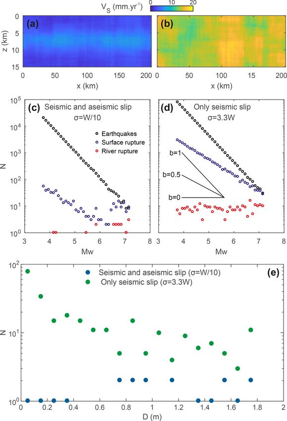
684                                                   P. Steer et al.: Statistical modelling of co-seismic knickpoint formation

around ∼ 10−1 m year−1 , in the central Apennines, Italy, and
in the Hatay Graben, southern Turkey (Whittaker and Boul-
ton, 2012), between ∼ 10−3 and ∼ 10−2 m year−1 . How-
ever, on shorter timescales, significantly higher rates can
be found with values potentially reaching ∼ 100 or even
∼ 101 m year−1 . For instance, Niagara Falls retreated at a
rate of a few metres per year over tens of years (Gilbert,
1907) and some knickpoints formed by the 1999 Chi-Chi
earthquake in Taiwan even retreated by a few hundreds of
metres over about 10 years (Yanites et al., 2010; Cook et al.,
2013). A more extensive analysis of the range of knickpoint
retreat rates in relation to the observation timescale can be
found in Van Heijst and Postma (2001) and in Loget and Van
Den Driessche (2009).
   In detachment-limited conditions, the stream power in-
cision model predicts that knickpoint horizontal migration
or retreat follows a linear or non-linear kinematic wave in
the upstream direction, depending on the slope exponent           Figure 1. Schematic sketch showing the model setup. The fault
(e.g. Rosenbloom and Anderson, 1994; Tucker and Whip-             plan, dipping with an angle θ , is represented by a red contour and in-
                                                                  cludes the earthquakes and their ruptures represented by a grey box,
ple, 2002; Whittaker and Boulton, 2012; Royden and Per-
                                                                  whose colour indicates the magnitude. The fault trace is aligned
ron, 2013). This prediction is supported by the apparent
                                                                  along the x axis and earthquakes occur at depth z. The river pro-
correlation between retreat rate and drainage area or water       file is indicated by a blue line along the y axis and has an elevation
discharge, deduced from field observation and experimen-          h. The river contains several knickpoints. Note that in this paper we
tal studies (Parker, 1977; Schumm et al., 1987; Rosenbloom        only focus on knickpoints occurring in near-fault condition. The rate
and Anderson, 1994; Bishop et al., 2005; Crosby and Whip-         of fault slip is VF , while knickpoints migrate at a constant velocity
ple, 2006; Loget et al., 2006; Berlin and Anderson, 2007).        (VR ).
However, some experimental results show no dependency of
retreat rate on water discharge (Holland and Pickup, 1976),
possibly due to the self-regulatory response of river geome-      of the differential topography associated with knickpoints.
try to water discharge through change in river channel width      However, transport-limited models are likely more pertinent
(Baynes et al., 2018). Other factors influencing retreat rate     to predict the evolution of fault scarps along hillslopes (e.g.
include, among others, sediment discharge (e.g. Jansen et         Rosenbloom and Anderson, 1994; Arrowsmith et al., 1996,
al., 2011; Cook et al., 2013), flood events (e.g. Baynes et       1998; Tucker and Whipple, 2002), and evidence points to-
al., 2015), rock strength (e.g. Stock and Montgomery, 1999;       ward a linear dependency on slope for knickpoint erosion
Hayakawa and Matsukura, 2003; Baynes et al., 2018), frac-         (Lague, 2014). Yet, the transformation of fault activity and
ture density and orientation (Antón et al., 2015; Brocard         slip during earthquakes to knickpoints and hillslope scarps
et al., 2016) and the spacing and height of the waterfalls        and their preservation throughout their subsequent erosion
(Scheingross and Lamb, 2017).                                     and retreat remains a challenging issue.
   Preservation of knickpoint shape during retreat is poorly
understood as very little data exist on the temporal evolution    3     Methods
of their shape. For instance, knickpoints along the Atacama
Fault System are systematically reduced in height compared        3.1    Fault setting
to the height of ruptures directly on the fault scarp (Ewiak
                                                                  The tectonic setting considered here is the one of a typical
et al., 2015). On the contrary, 10 years after Chi-Chi earth-
                                                                  active intracontinental thrust fault, able to generate earth-
quake, the height of co-seismic knickpoints ranged from 1 to
                                                                  quakes up to magnitude 7.3. The thrust fault has a length
18 m (Yanites et al., 2010), while the initial surface rupture
                                                                  L = 200 km, a width W = 30 km and a dip angle θ = 30◦ so
was limited to 0.5 to 8 m in height (Chen et al., 2001). The-
                                                                  that the fault tip is located at a 15 km depth. The duration
oretically, only the stream power model with a linear depen-
                                                                  of the simulation T is set to 10 kyr to cover many seismic
dency on slope predicts the preservation of knickpoint shape,
                                                                  cycles and for earthquakes to be well distributed along the
favoured by a parallel retreat (e.g. Rosenbloom and Ander-
                                                                  finite fault plane. A schematic sketch illustrates the model
son, 1994; Tucker and Whipple, 2002; Royden and Perron,
                                                                  setup (Fig. 1).
2013). A less-than-linear dependency on slope leads to con-
cave knickpoints, while a more-than-linear dependency on
slope leads to convex knickpoints. Transport-limited models
that reduce to advection–diffusion laws lead to a diffusion

Earth Surf. Dynam., 7, 681–706, 2019                                                     www.earth-surf-dynam.net/7/681/2019/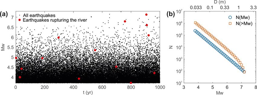
P. Steer et al.: Statistical modelling of co-seismic knickpoint formation                                                    685

3.2   Mainshocks                                                  of Omori’s law that controls the spatial distribution of after-
                                                                  shocks (Helmstetter and Sornette, 2003). The BASS model
Mainshocks are generated along the fault plane. The po-           relies on six parameters: the b value that we set equal to
tential magnitude range of mainshocks is bounded by fault         b = 1, the magnitude difference 1Mw = 1.25 of Båth’s law,
width, which sets the maximum earthquake rupture width            the exponent p = 1.25 and offset c = 0.1 d of the temporal
and by a minimum rupture width, here chosen as 500 m.             Omori law, and the exponent q = 1.35 and offset d = 4.0 m
Based on Leonard (2010), the modelled thrust fault allows         of the spatial Omori law. The values of these aftershock pa-
magnitudes ranging from Mwmin = 3.7 to Mwmax = 7.3. In-           rameters are based on Turcotte et al. (2007) and are constant
side these bounds, the magnitude of each mainshock is de-         for all the simulations performed in this paper. Seismicity
termined by randomly sampling the Gutenberg–Richter dis-          along the fault is therefore made of mainshocks and their af-
tribution, with a b value of 1 (Fig. 2). The earthquake pro-      tershocks. This aftershock model is also similar to the one
ductivity of the distribution is inferred based on the arbi-      developed by Croissant et al. (2019).
trarily chosen rate of mainshock (R = 0.1 d−1 ), leading to
a = log10 (R T ) + b Mwmin = 8.975. The time occurrence of
each mainshock is randomly sampled over the duration of the       3.4   Earthquake rupture
simulation. Each mainshock is therefore considered indepen-       The length Lrup , width Wrup and average co-seismic dis-
dent, and the only relationship between mainshocks is that        placement D of each earthquake rupture, including main-
their population statistically respects the Gutenberg–Richter     shocks and aftershocks, are determined using scaling laws
distribution (Gutenberg and Richter, 1944).                       with seismic moment MO , empirically determined from a set
   The spatial location of mainshocks inside the fault plane      of intraplate dip-slip earthquakes (Leonard, 2010) following
is sampled using a 2-D distribution that corresponds to a         Eqs. (2)–(4):
truncated normal distribution across-strike and to a uniform
distribution along-strike (Fig. 3). A normal distribution with                           !      2
                                                                                             3(1+β)
depth roughly mimics the depth distribution of natural earth-                    MO
                                                                  Lrup =          3/2
                                                                                                      ,                       (2)
quakes in the upper crust, which tends to show a maximum                        µC1 C2
number of earthquakes at intermediate depth and less to-                          β
                                                                  Wrup = C1 Lrup ,                                            (3)
wards the top and the tip of the fault (e.g. Sibson, 1982;
                                                                            1     1+β
Scholz, 1998). Therefore, we set the mean of the normal dis-                2
                                                                  D = C1 C2 Lrup , 2
                                                                                                                              (4)
tribution equal to a 7.5 km depth as the fault tip has a 15 km
depth, so earthquakes are more numerous at this intermedi-        where C1 = 17.5, C2 = 3.8 × 10⁻⁵ and β = 2/3 are con-
ate depth. We define two end-member models, referred to as        stants, and µ = 30 GPa is the shear modulus (Fig. 1). The
(1) the “seismic and aseismic slip” model using a variance of     locations of the rupture patches around each earthquake are
the normal distribution σ = W/10, corresponding to a nar-         positioned randomly to prevent hypocentres being centred
row depth distribution, and (2) the “only seismic slip” model     inside their rupture patches. The fault has some periodic
with σ = 3.3 W , corresponding to an almost uniform depth         boundary conditions, in the sense that if the rupture patch of
distribution. We impose that the maximum earthquake fre-          an earthquake exceeds one of the fault limits, the rupture area
quency, at depth 7.5 km, is equal in between all the models.      in excess is continued on the opposite side of this limit. This
                                                                  choice maintains a statistically homogeneous pattern of fault
3.3   Aftershocks                                                 slip rate on the fault plane in the case of the “only seismic
                                                                  slip” model (which displays an almost homogeneous distri-
Each mainshock triggers a series of aftershocks that is deter-    bution of mainshocks on the fault plane). Another strategy,
mined based on the BASS model (Turcotte et al., 2007). It         consisting in relocating each rupture in excess inside the fault
represents an alternative to the more classical epidemic-type     limits, was dismissed as it was leading to gradients of fault
aftershock sequence (ETAS) models (Ogata, 1988), with the         slip rates close to fault tips.
advantage of being fully self-similar. We here only briefly de-
scribe the BASS model, as more details can be found in Tur-       3.5   Seismic and aseismic slip
cotte et al. (2007). Based on a mainshock, the BASS model
produces a sequence of aftershocks which respect four statis-     Slip along the fault plane is partitioned between seismic and
tical laws: (1) the Gutenberg–Richter frequency–magnitude         aseismic slip. The average slip rate VF of the fault over
distribution (Gutenberg and Richter, 1944; Fig. 1); (2) a mod-    the duration Pof the simulation is given by VF = VS + VA ,
ified Båth’s law (Shcherbakov and Turcotte, 2004), which          where VS = MO / (µTWL) is the seismic slip, due to all
controls the difference in the magnitude of a mainshock and       the earthquakes rupturing the fault, and VA is aseismic slip.
its largest aftershock; (3) a generalized form of Omori’s         The average degree of seismic coupling on the fault plane is
law describing the temporal decay of the rate of after-           χ = VS /VF (Scholz, 1998) and represents the proportion of
shocks (Shcherbakov et al., 2004); and (4) a spatial form         fault slip that occurs by earthquakes and seismic slip. We

www.earth-surf-dynam.net/7/681/2019/                                                     Earth Surf. Dynam., 7, 681–706, 2019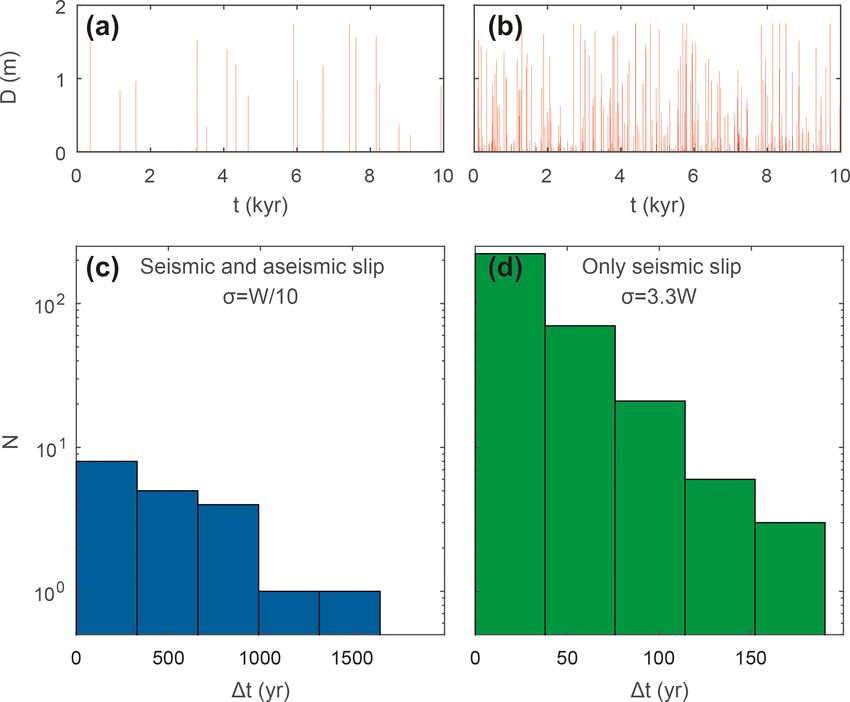
686                                                       P. Steer et al.: Statistical modelling of co-seismic knickpoint formation

Figure 2. Modelled seismicity and its statistical characteristics. (a) Time distribution t of the magnitude Mw of earthquakes during the
first 1000 years of one model. Both mainshocks and aftershocks are shown with black dots. Earthquakes with rupture zone extending to
the surface and cutting the river, located at the middle of the fault trace, are shown with red dots. (b) The cumulative (light red squares)
and incremental (light blue circles) Gutenberg–Richter frequency–magnitude distribution of earthquakes for one model. N is the number of
events and D is the associated displacement computed using the Leonard (2010) scaling law.

Figure 3. Depth distribution of earthquakes, seismic and aseismic slip. (a) Depth distribution of the number N of mainshocks for the two
models considered here. The depth distribution is a normal one centred at a 7.5 km depth and with a variance σ equal to W/10 (blue) or
3.3 W (green). (b) Depth distribution of seismic VS slip. The vertical black line indicates the averaged fault slip rate of ∼ 15 mm year−1 ,
summing seismic and aseismic slip. Aseismic slip rate is simply the difference between the average fault slip rate and seismic slip rate, so
that all models share the same total slip rate.

define the reference fault slip rate as equal to the seismic            an average value of ∼ 15 mm year−1 . However, these spa-
slip rate of the “only seismic slip” model so that VF = VS '            tial variations are randomly distributed and do not follow any
15 mm year−1 . This velocity is only given approximatively,             specific pattern (Fig. 4).
as the model developed here is stochastic and leads to intrin-
sic variability in the number and magnitude of earthquakes
                                                                        3.6    River uplift
for the same parametrization. We follow the paradigm of sta-
tistically homogeneous long-term fault slip over the fault.             A virtual river, orientated orthogonally to the fault trace,
The “only seismic slip” model, with an almost uniform spa-              crosses the fault trace at its centre, at x = L/2. This river wit-
tial distribution of mainshocks, is therefore on average fully          nesses the distribution of co-seismic and aseismic displace-
coupled, with χ = 1, while the “seismic and aseismic slip”              ment modifying its topography and slope. For the sake of
model, displaying a large change with depth of the distri-              simplicity, we assume that (1) any surface rupture generates
bution of mainshocks, is dominated by aseismic slip with                displacement only in the vertical direction and (2) that co-
χ ' 0.25. In the modelling framework developed here, even               seismic and aseismic deformation lead to a block uplift of
a fully coupled fault can display significant spatial variations        the hanging wall, homogeneous along the river profile. These
of fault slip rate. Slip rate on the fault plane of the “only seis-     two assumptions clearly neglect the influence of the fault dip-
mic slip” model varies between 11.4 and 18.2 mm year−1 for              ping angle and of the spatial distribution of uplift in surface

Earth Surf. Dynam., 7, 681–706, 2019                                                          www.earth-surf-dynam.net/7/681/2019/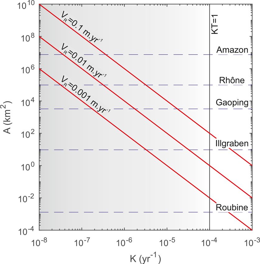
P. Steer et al.: Statistical modelling of co-seismic knickpoint formation                                                           687

                                                                        3.7    River topographic evolution
                                                                        To model river erosion, we consider a simple model consid-
                                                                        ering that knickpoints migrate upstream at constant velocity
                                                                        VR along the y axis, which is perpendicular to the fault trace
                                                                        orientated along the x axis. We show in Appendix A that
                                                                        this constant migration velocity model corresponds to a pre-
                                                                        diction of the stream power law (Howard and Kerby, 1983;
                                                                        Howard et al., 1994; Whipple and Tucker, 1999; Lague,
                                                                        2014) which holds if drainage area is about constant over
                                                                        the region of interest. Our model is therefore appropriate
                                                                        to model knickpoint migration in near-fault conditions and
                                                                        for large drainage areas. In the following, we only consider
                                                                        the migration of slope patches over short distances upstream,
                                                                        during the T = 10 kyr of the simulation. We set the horizon-
                                                                        tal retreat rate to VR = 0.1 m year−1 , which corresponds to
                                                                        a high rate of knickpoint retreat over geological timescales
                                                                        (> 103 years) but a moderate one over shorter timescales
                                                                        (e.g. Van Heijst and Postma, 2001).

                                                                        3.8    Numerical implementation
                                                                        Numerically, we solve in 2-D the evolution of a river pro-
                                                                        file crossing a fault, subjected to slip during earthquakes and
                                                                        to aseismic slip. After having set the parameters, the model
                                                                        (1) generates mainshocks and aftershocks, including their
                                                                        magnitude, location and timing, and (2) computes the time
                                                                        evolution of the river profile subjected to uplift and erosion.
                                                                        Time stepping combines a regular time step, to account for
                                                                        uplift by aseismic slip, with the time of occurrence of each
                                                                        earthquake rupturing the surface at the location of the river, to
Figure 4. Incremental distribution of earthquake magnitude and          account for co-seismic slip. During each aseismic time step,
displacement in surface and at depth. Maps of averaged fault seis-      one node of coordinates (h = 0, y = 0) is added to the river
mic slip rate VS on the fault plane for (a) the “seismic and aseis-     profile at the downstream end of the river (i.e. the location of
mic slip” and (b) the “only seismic slip” models. The scale of the      the fault trace). During each co-seismic time step, two nodes
z axis is increased compared to the x axis to enhance readability.      of coordinates (h = 0, y = 0) and (h = D, y = 0) are added
(c–d) Modelled magnitude distributions of earthquakes on the fault      to the river at the downstream end of the river, to represent
(black circles), earthquakes rupturing the surface (blue circles) and   the vertical step associated with the co-seismic knickpoint.
of earthquakes rupturing the river (red circles) for the same models
                                                                        The remaining nodes, located upstream, are uplifted follow-
as in panels (a) and (b), respectively. Here, N is the incremental
                                                                        ing the aseismic uplift rate VA and potential co-seismic dis-
number of earthquakes, i.e. N(m). (e) Distributions of displacement
for earthquake rupturing the river for the considered models, with      placement. River erosion is accounted for by horizontal ad-
green and blue circles representing the “only seismic slip” and the     vection of river nodes following a constant velocity VR along
“seismic and aseismic slip” models, respectively.                       the y axis. As we neglect the contribution of horizontal dis-
                                                                        placement due to fault slip, we do not consider any horizon-
                                                                        tal advection induced by tectonics, contrary to some previous
during an earthquake, which depends mainly on earthquake                studies (Miller et al., 2007; Castelltort et al., 2012; Thieulot
magnitude, depth, geometry and the crustal rheology. In turn,           et al., 2014; Goren et al., 2015).
earthquakes that do not rupture the surface at the location of
the river have no effect on river topography and slope in this          4     Magnitude, displacement and temporal
simple model. The rate of uplift is equal to VF at the intersec-              distributions of earthquakes and co-seismic
tion between the fault trace and the river.                                   knickpoints

                                                                        4.1    Magnitude distributions
                                                                        We first use this model to investigate the distribution of earth-
                                                                        quake magnitudes that rupture (1) the fault, (2) the surface

www.earth-surf-dynam.net/7/681/2019/                                                         Earth Surf. Dynam., 7, 681–706, 2019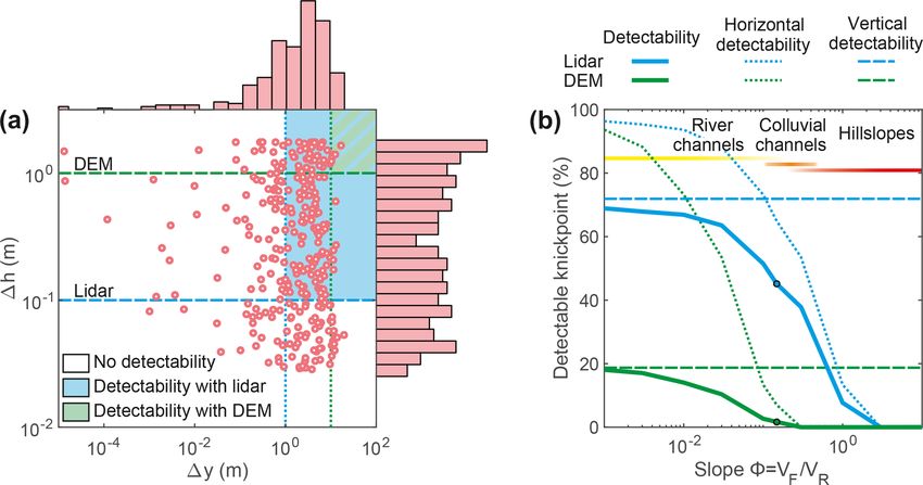
688                                                    P. Steer et al.: Statistical modelling of co-seismic knickpoint formation

and (3) the surface at the location of the river (Fig. 4). For
clarity, the frequency–magnitude distributions are shown as
incremental distributions N (m) and not as cumulative distri-
butions N (≥ m). Unsurprisingly, the frequency–magnitude
distribution of earthquakes on the fault follows a negative
power-law distribution with an exponent of b = 1, follow-
ing the imposed Gutenberg–Richter distribution. Increasing
the degree of seismic coupling χ only shifts the distribution
vertically by increasing the total number of earthquakes.
   The distribution of earthquakes rupturing the surface fol-
lows a negative power law with an exponent of −0.5 for the
“only seismic slip” model with a high degree of seismic cou-
pling. In the case of the “seismic and aseismic slip” model,
characterized by a lower degree of seismic coupling, the dis-
tribution follows a more complex pattern. Below a threshold
magnitude, here around 6, the distribution follows a nega-
tive power law with an exponent of −0.5. Above this thresh-
old magnitude, the distribution rises to reach the Gutenberg–
                                                                   Figure 5. Time distribution of earthquakes rupturing the river. (a–
Richter distribution and then decreases following the trend
                                                                   b) Co-seismic displacements D at the location of the river as a func-
of the Gutenberg–Richter distribution. This results from the
                                                                   tion of time t for each model. (c–d) Distribution of inter-event time
non-uniformity of the distribution of earthquakes with depth.      1t of earthquakes rupturing the surface at the location of the river.
In this model, large-magnitude earthquakes can rupture the
surface, without requiring their hypocentres to be at shallow
depth, whereas small-magnitude earthquakes can only rup-           4.2   Displacement distributions
ture the surface if their hypocentres are located close to the
surface, which is unlikely due to the shape of the depth dis-      Fault displacement D during an earthquake scales linearly
tribution of mainshocks (Fig. 3). The threshold magnitude          with seismic moment MO (Wells and Coppersmith, 1994;
depends on the depth distribution of mainshocks, and par-          Leonard, 2010), which is related to magnitude by a log-
ticularly on its upper limit but also on the aftershock depth      arithmic function, Mw = 2/3log10 (MO ) − 6.07 (Kanamori,
distribution that extends the range of possible depths due to      1977). It results that a uniform distribution of earthquake
Omori’s law in space.                                              magnitude, that is observed for earthquakes cutting the river
   The distribution of earthquake magnitude rupturing the          in the case of the “only seismic slip” model, should lead to
river follows a uniform distribution for the “only seismic         a negative exponential distribution of earthquake displace-
slip” model. This novel result has potentially large implica-      ments. The same finding exists with the numerical model
tions as it means that a river has an equal probability of being   (Fig. 4e). In the case of the “seismic and aseismic slip”
ruptured by large or small earthquakes. This homogeneous           model, it is more difficult to quantitatively characterize the
distribution results from considering earthquake ruptures at       resulting distributions due to the lack of events, but we ob-
one location and is yet consistent with a Gutenberg–Richter        serve a relatively uniform distribution of surface displace-
distribution of magnitudes along the modelled 2-D fault            ments.
plane. However, for the “seismic and aseismic slip” model,
mostly large-magnitude earthquakes manage to have ruptures         4.3   Temporal distributions
cutting the river profile. Low-magnitude earthquakes, except
for a few events, do not rupture the river. The magnitude          We now investigate the time distribution of earthquakes rup-
threshold for river rupture is close to 6, similar to the one      turing the surface at the location of the river and their as-
observed for surface ruptures. To date, there is no univer-        sociated displacement. The “seismic and aseismic slip” and
sal model of the depth distribution of earthquakes and of          the “only seismic slip” models have 20 and 299 earthquakes
the partitioning between aseismic and seismic slip at shallow      cutting the river, respectively. Their average co-seismic dis-
depth for intra- or inter-plate faults (e.g. Marone and Scholz,    placement is 1 and 0.5 m, respectively. This illustrates that
1988; Scholz, 1998, Schmittbuhl et al., 2015; Jolivet et al.,      models dominated by aseismic slip have less frequent earth-
2015). Yet, our results, i.e. a uniform distribution of earth-     quakes cutting the river but that their average displacement
quake magnitude cutting the river in the fully seismic case or     is greater, due to the censoring of surface ruptures associated
only large-magnitude earthquakes rupturing the river for the       with low-magnitude earthquakes (Fig. 4).
model dominated by aseismic slip at shallow depth, clearly            Consistent with this last result, the inter-event time 1t in
offer a guide to analyse river profiles in terms of fault prop-    between successive earthquakes cutting the river increases
erties.                                                            significantly from the “only seismic slip” model to the most

Earth Surf. Dynam., 7, 681–706, 2019                                                     www.earth-surf-dynam.net/7/681/2019/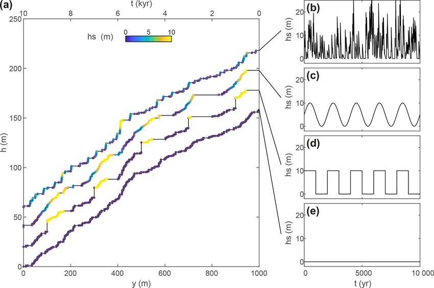
P. Steer et al.: Statistical modelling of co-seismic knickpoint formation                                                        689

“seismic and aseismic slip” model. In other words, the fre-
quency of surface rupture is higher in the most seismic mod-
els and decreases with aseismic slip. This inter-event time
distribution follows for each model an exponential decay
(Fig. 5), which is consistent with a Poisson process. For the
“seismic and aseismic slip” model, the low number of events,
20 earthquakes, precludes characterizing a negative exponen-
tial distribution. This exponential decay implies that fault
properties have no major effect on the temporal structure of
earthquakes cutting a river, only on their frequency.

5     Knickpoints along single river profiles

5.1    Constant knickpoint velocity

If the slope patches generated by differential motion across
the fault do not migrate horizontally, due to, for instance, a
lack of erosion, the succession of earthquakes would pro-
gressively build a vertical fault scarp in this model. Here,
we rather consider the case of a migrating topography due
to river backward erosion following a kinematic model with
                                                                    Figure 6. Modelled river profiles considering the “only seismic
VR = 0.1 m year−1 . It results in an averaged river slope just
                                                                    slip” (green line) and the “seismic and aseismic slip” (blue line)
upstream the fault trace of ϕ = VF /VR = 0.15 or 8.5◦ , with        models. For the latter, the contribution of seismic slip is shown
VF = 15 mm year−1 (see Appendix A and Fig. A1). River               (dashed blue line).
profiles are obtained for the two different models (Fig. 6). We
first only consider seismic slip, so that only earthquakes rup-
turing the river contribute to topographic building. After T =      height, 1h0 = 1 m a reference knickpoint height and r = 0.1
10 kyr of model duration, the models have resulted in about         an exponent representing the sensitivity of knickpoint veloc-
20 to 150 m of topographic building for the “seismic and            ity to knickpoint height. This model is motivated by mechan-
aseismic slip” and “only seismic slip” models, respectively.        ical arguments suggesting a dependency of knickpoint veloc-
The local ratio between VS and VF can depart from their             ity to their height (Scheingross and Lamb, 2017). We allow
fault-averaged values χ, due (1) to the non-homogeneous             a quicker knickpoint of height 1hi that encounters slower
distribution of co-seismic slip on the fault for models with        knickpoints of height 1hj to merge, forming in turn a sin-
significant aseismic slip and (2) to the stochasticity of each      gle knickpoint of height 1hi + 1hj and of greater speed
model. For instance, the “seismic and aseismic slip” model          than the former knickpoints. The resulting river profile can
shows an apparent ratio of 20/150 ' 0.13 compared to its av-        be compared to the one obtained with the “only seismic
erage value of χ = 0.25. Each successive co-seismic knick-          slip” model (Fig. 7a). The dependency of knickpoint speed to
point is separated by a flat river section, due to the absence of   height leads to a river profile with high but fewer knickpoints.
slope building by aseismic slip. As expected, the “only seis-       The interdistance between successive knickpoints increases
mic model” displays a larger number of co-seismic knick-            with total retreat. Small knickpoints only survive close to the
point than the aseismic model. Adding aseismic slip leads to        fault before being “eaten” by quicker and higher knickpoints
sloped reaches between each knickpoint (Fig. 6), with slopes        during their retreat. Only the highest knickpoints, reaching
equal to VA /VF . There is obviously a larger slope variabil-       tens of metres in height, survive after a significant distance
ity in the models dominated by seismic slip due to a larger         of retreat. This behaviour is also evidenced when comparing
number of knickpoints.                                              the distributions of knickpoint heights for these two models
                                                                    (Fig. 7b). The dependency of knickpoint velocity to height
5.2    Knickpoint velocity that depends on knickpoint               leads to very few knickpoints, with however a large propor-
       height                                                       tion of them having a metric or decametric scale. This high-
                                                                    lights that even limited non-linearities in the knickpoint re-
Even if most simulations of this paper are done with a sim-         treat model can lead to river profiles with significant differ-
ple kinematic model using a constant knickpoint velocity,           ences.
we now consider a model with a knickpoint velocity that
depends on knickpoint height with VR = r(1 + 1h/1h0 )q ,
where d is a constant, set to the previously used constant
knickpoint retreat rate of 0.1 m year−1 , 1h the knickpoint

www.earth-surf-dynam.net/7/681/2019/                                                      Earth Surf. Dynam., 7, 681–706, 2019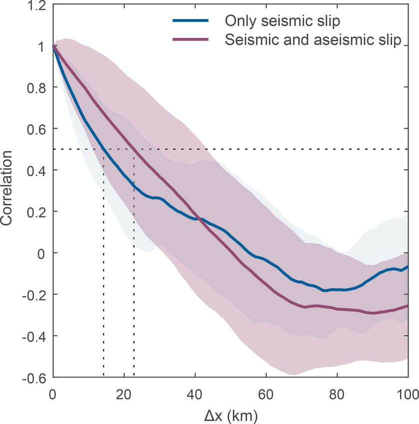
690                                                         P. Steer et al.: Statistical modelling of co-seismic knickpoint formation

Figure 7. Modelled (a) river profiles and (b) knickpoint height distribution considering a constant knickpoint velocity (green line and circles)
or a velocity depending on knickpoint height (red line and circles).

5.3   Sediment cover, fault burial and knickpoint formation               are purely illustrative and do not aim at offering an accurate
                                                                          description of the impact of tectonic or climatic changes on
We have neglected up to now the role of sediments and                     sediment cover dynamics. For each scenario, except the one
their impact on knickpoint formation. More specifically, fault            with no sediment cover, the mean sediment thickness is 5 m.
scarps can remain buried during the aggradation phase of                  For the sake of simplicity, we only consider the “only seismic
an alluvial fan located immediately downstream of the fault               slip” model with the same temporal sequence of earthquakes
(e.g. Carretier and Lucazeau, 2005). This mechanism is sug-               in each of the four scenarios. Knickpoint velocity is kept con-
gested to be a primary control of knickpoint and water-                   stant and equal to VR = 0.1 m year−1 .
fall formation by allowing the merging of several small co-                  The square-wave model is useful to assess the impact of
seismic scarps formed during burial phases into single high-              abrupt changes in sediment thickness. During the phase of
elevation waterfalls that migrate during latter incision phases           a high sediment cover thickness that lasts 2000 years, the
(Finnegan and Balco, 2013; Malatesta and Lamb, 2018). We                  scarp progressively builds its height until it reaches 10 m dur-
test this mechanism and its impact on river profiles using a              ing successive fault ruptures. Over this period, there is no
simple description of fault burial by sediment cover (Fig. 8).            knickpoint formation, while previously formed knickpoints
At each time step, the formation of a knickpoint can only                 continue to migrate upstream, leading to elongated flat river
occur if the fault scarp height, h(y = 0), is greater than the            reaches upstream of the fault. Once the scarp is re-exposed,
sediment thickness of the alluvial fan, hs . In this case, the            the following earthquakes generate knickpoints (yellow dots
formed knickpoint height is simply h (y = 0) − hs .                       in Fig. 8a), with their individual height corresponding to
   Temporal variations of sediment thickness are prescribed               each associated earthquake displacement. Then, the abrupt
using four scenarios: (1) no sediment cover, hs = 0, corre-               transition from 10 m of sediment thickness to no sediment
sponding to the reference model (Fig. 8e); (2) a square-wave              thickness suddenly exposes 10 m or more of fault scarp that
(or step-like) function with a periodicity of 2000 years and a            forms a migrating knickpoint of elevation much higher than
maximum amplitude of 10 m (Fig. 8d); (3) a sinusoidal func-               the largest earthquake displacement, i.e. 1.8 m. Then, dur-
tion with a periodicity of 2000 years and a maximum am-                   ing the 2000 years that follow, with no sediment cover, each
plitude of 10 m (Fig. 8c); and (4) an earthquake-driven sed-              earthquake rupture generates a new knickpoint (blue dots in
iment cover, where sediment increases instantaneously after               Fig. 8), as in the reference model.
each earthquake that ruptures the river with an amplitude ar-                The sinusoidal model, mimicking climatic oscillations
bitrarily defined proportional to (Mw − 5)2 , followed by a               (Fig. 8c), displays a relatively similar behaviour, except that
linear decrease over 100 years, following results by Crois-               it does not form 10 m high knickpoints during the phase
sant et al. (2017) (Fig. 8b). This last scenario mimics, in a             of degradation of the sediment cover. Instead, this phase
very simplified manner, the potential transient response of an            leads to the formation of “climatic knickpoints” as the rate
alluvial fan to the observed increase of river sediment load              of decrease in sediment thickness is greater than the rate
induced by earthquake-triggered landslides (Hovius et al.,                of scarp building by fault slip. For the exact same reason,
2011; Howarth et al., 2012; Croissant et al., 2017). Alterna-             the phase of sediment aggradation is characterized by no
tively, the periodic scenario mimics the potential response of            knickpoint formation and by flat river reaches. Knickpoint
sediment thickness to some climatic cycles. These scenarios               formation and the signature of the river profile are there-

Earth Surf. Dynam., 7, 681–706, 2019                                                             www.earth-surf-dynam.net/7/681/2019/
P. Steer et al.: Statistical modelling of co-seismic knickpoint formation 691
Figure 8. Impact of fault burial by sediment cover on river profile. (a) River profiles are generated with no sediment cover (hs = 0; see panel
e), with step-like temporal variations for sediment cover with a periodicity of 2000 years (see panel d), with sinusoidal temporal variations
for sediment cover with a periodicity of 2000 years, mimicking climatic changes (see panel c), with a temporal variation of sediment cover
induced by earthquakes (see panel b). The mean sediment cover thickness, hs , is equal to 5 m in panels (b), (c) and (d). River profiles are
indicated with black lines and the sediment cover thickness at the time of knickpoint formation is indicated by the colour of the points. For
readability, the river profiles are shifted by 20 m on panel (a).
fore dominated by the climatic signal controlling sediment 6 Knickpoints along successive parallel rivers
aggradation–degradation phases rather than by fault slip.
In these scenarios, the fault-burial mechanism by sediment 6.1 From single to several parallel rivers
cover does not necessarily lead to knickpoints with elevation
greater than earthquake ruptures, except for abrupt removals We now explore the degree of spatial correlation in be-
of sediment cover such as in the square-wave model. Yet, in tween the topographic profiles of several parallel rivers flow-
all these models, the fault-burial mechanism limits the pe- ing in an across-strike manner along the fault trace. For the
riods of differential topography building, leading in turn to sake of simplicity, we ignore the role of sediment cover on
succession of steepened river reaches or knickzones, corre- knickpoint formation and use a constant knickpoint veloc-
sponding to periods of sediment removal, alternating with ity. Paleo-seismological studies using knickpoints to infer
low slope river reaches, corresponding to periods of sedi- fault activity generally consider the distributions of knick-
ment aggradation. Figure 9 illustrates the role of sediment points along several subparallel rivers to lead to statistically
cover in modulating the surface expression of tectonics and robust analyses and to assess the spatial extent of each past
co-seismic displacement. For the highest rates of sediment earthquake (e.g. Ewiak et al., 2015; Wei et al., 2015; Sun et
aggradation and removal, river profiles are dominated by the al., 2016). Correlating topography and knickpoints along the
temporal evolution of the sediment cover and not by the ac- strike of a fault, using parallel rivers, also offers independent
tivity of the fault, whereas for limited sediment aggradation means to assess the rupture length and the magnitude of a
and removal rates, the river profiles and the succession of past earthquake. Using multiple rivers is also less likely to
knickpoints are dominated by the temporal occurrence of be biased by potential heterogeneities occurring along single
earthquakes and not by the temporal evolution of the sedi- rivers.
ment cover. These results are consistent with the ideas devel- We therefore consider a set of rivers separated by 1x =
oped by Malatesta and Lamb (2018). 1 km along the strike of the fault, i.e. the x direction. Because
(1) the drainage area of each of these rivers can vary by or-
ders of magnitude and (2) because knickpoint retreat rates
show a high variability, their knickpoint migration rate VR is
randomly sampled in the range 0.001 to 0.1 m year−1 . Each
profile of the 200 rivers shares some common topographic
characteristic, including their average number of knickpoints
www.earth-surf-dynam.net/7/681/2019/ Earth Surf. Dynam., 7, 681–706, 2019692 P. Steer et al.: Statistical modelling of co-seismic knickpoint formation
and total elevation (Fig. 10). However, their average slopes
and the horizontal position y of the knickpoints largely dif-
fer due to the variability of VR . Knowing a priori VR and the
duration T of the simulation (i.e. the age of the knickpoints)
enables to define a normalized horizontal position relative
to the fault, y/(T VR ). Practically, several studies normalized
distance by the square root of drainage area, as drainage area
is generally used as a proxy for retreat rate (e.g. Crosby and
Whipple, 2006). Knickpoints generated at the same time,
along different rivers with different retreat rates, share the
same normalized distance relative to the fault. This represen-
tation is convenient to assess the spatial extent of an earth-
quake rupturing several rivers along-strike. Non-normalized
river profiles are shown in Fig. B1.
6.2 Knickpoint correlation in between several parallel
rivers crossing the fault
This representation is convenient to assess the degree of cor-
relation of the profiles of the successive rivers. Obviously,
there is no significant topographic correlation when consid-
ering rivers with such a high variability in retreat rates, e.g.
0.001 to 0.1 m year−1 . We therefore compute the matrix of
correlation between each river elevation profile using the
river normalized horizontal distance (Fig. B1). River eleva-
tion is corrected or “detrended” from its average slope to re-
move an obvious source of topographic correlation. We then
compute the average coefficient of correlation for a given
river interdistance 1x ranging from 0 to 100 km (Fig. 11).
The two models, the “only seismic slip” and the “seismic and
aseismic slip” models, show a similar pattern, with a signif-
icant positive correlation (> 0.5) for rivers separated by less
than 14 to 23 km (10 to 45 km if accounting for the standard
deviation). The maximum distance over which a correlation
is significant corresponds to about 35 km, half the maximum
co-seismic rupture length of ∼ 70 km along the considered
fault. This illustrates that knickpoints should not be corre-
lated for rivers separated by more than this distance, consid-
ering the tectonic setting of this model, and fault dimensions.
This correlation distance could increase using a wider fault
generating larger-magnitude earthquakes with longer surface
Figure 9. Impact of the rate of sediment aggradation and fault rupture. We also find that the correlation is better for the
burial on river profile. (a) River profile simulated with sinu- model dominated by aseismic slip and showing less knick-
soidal temporal variations for sediment cover, mimicking climatic
points (Fig. B1). Positive correlations were obtained using
changes, with a periodicity of 2000 years, and an amplitude of 0, 1,
horizontal distance normalized by retreat rate. However, us-
2.5, 5, 10 and 20 m. River profiles are indicated with black lines and
the sediment cover thickness at the time of knickpoint formation is ing only catchments with similar retreat rates would also lead
indicated by the colour of the points. (b) Time evolution of the sed- to positive and significant correlation even when using non-
iment cover hs for the different simulations presented in panel (a). normalized distance.
(c) Co-seismic displacements D at the location of the river as a func-
tion of time t for each model. For panels (a), (b) and (c), the x axis
7 Knickpoint detectability
indicates both the distance y along the river and the correspond-
ing time t, to visually relate fault displacement, sediment cover and
river profile. Time and distance along the river are related through 7.1 Knickpoint detectability for the reference model
the knickpoint retreat rate, VR = yt . River profiles are used in many studies to extract co-seismic
knickpoints and to assess fault activity and local-to-regional
Earth Surf. Dynam., 7, 681–706, 2019 www.earth-surf-dynam.net/7/681/2019/P. Steer et al.: Statistical modelling of co-seismic knickpoint formation 693 Figure 10. Topography of a set of parallel rivers flowing in an across-strike manner along the fault. (a–b) River profiles of 200 rivers separated by 1 km along the strike of the fault, i.e. the x direction. River elevation h is given along the same axis, with a scaling factor of 1000. River length y across the strike of the fault is normalized by knickpoint migration rate VR times the duration of the simulation T . Non-normalized river profiles are shown in Fig. B1. The colour scale is only present to help figure readability. seismic hazard (e.g. Ewiak et al., 2015; Wei et al., 2015; Sun with precision not better than a few metres. Local-to-regional et al., 2016). It is therefore required to investigate whether topographic datasets obtained from current airborne lidar or modelled knickpoints are statistically detectable. Knickpoint photogrammetric data or derived from aerial or satellite im- detection often relies on the use of digital elevation models agery (e.g. Pléiades) display a resolution between 0.5 and and topographic data (e.g. Neely et al., 2017; Gailleton et about 1–5 m and a typical vertical precision of 10 cm above al., 2019), which are obtained at a certain scale or resolu- water. Moreover, in the vertical direction, knickpoint de- tion. The detectability of each individual knickpoint depends tectability depends also on the inherent bed roughness, mean not only on its distance to its adjacent knickpoints but also alluvial deposit thickness and the local distribution of sedi- on the horizontal resolution and vertical precision of the to- ment grain size. Sediment grains of dimension greater than pographic data and on the roughness of the riverbed. In the 0.1 m are commonly found in rivers located in mountain following, we consider that a knickpoint is detectable if its ranges (e.g. Attal and Lavé, 2006), especially at low drainage height is greater than the vertical precision of topographic areas, and there is often a thin layer of sediment covering the data and if its distance to adjacent knickpoints is greater than channel bed, potentially hiding bedrock features. If we fully the horizontal resolution of topographic data. acknowledge the role of river roughness, we focus here on Resolutions of topographic data available at the global the issue of detectability relative to topographic resolution scale (e.g. SRTM or ASTER) are between 10 and 100 m, www.earth-surf-dynam.net/7/681/2019/ Earth Surf. Dynam., 7, 681–706, 2019
You can also read