Using altimetry observations combined with GRACE to select parameter sets of a hydrological model in a data-scarce region
←
→
Page content transcription
If your browser does not render page correctly, please read the page content below
Hydrol. Earth Syst. Sci., 24, 3331–3359, 2020
https://doi.org/10.5194/hess-24-3331-2020
© Author(s) 2020. This work is distributed under
the Creative Commons Attribution 4.0 License.

Using altimetry observations combined with GRACE to select
parameter sets of a hydrological model in a data-scarce region
Petra Hulsman1 , Hessel C. Winsemius1 , Claire I. Michailovsky2 , Hubert H. G. Savenije1 , and Markus Hrachowitz1
1 WaterResources Section, Faculty of Civil Engineering and Geosciences, Delft University of Technology,
Stevinweg 1, 2628 CN Delft, the Netherlands
2 IHE Delft Institute for Water Education, Westvest 7, 2611 AX Delft, the Netherlands

Correspondence: Petra Hulsman (p.hulsman@tudelft.nl)

Received: 5 July 2019 – Discussion started: 10 September 2019
Revised: 10 April 2020 – Accepted: 27 May 2020 – Published: 30 June 2020

Abstract. Limited availability of ground measurements in          ing rating curves in the form of power relationships with
the vast majority of river basins world-wide increases the        two additional free calibration parameters per virtual station
value of alternative data sources such as satellite obser-        resulted in an overestimation of the discharge and poorly
vations in hydrological modelling. This study investigates        identified feasible parameter sets (ENS,Q,5/95 = −2.6–0.25).
the potential of using remotely sensed river water levels,        However, accounting for river geometry proved to be highly
i.e. altimetry observations, from multiple satellite missions     effective. This included using river cross-section and gradi-
to identify parameter sets for a hydrological model in the        ent information extracted from global high-resolution terrain
semi-arid Luangwa River basin in Zambia. A distributed            data available on Google Earth and applying the Strickler–
process-based rainfall–runoff model with sub-grid process         Manning equation to convert modelled discharge into wa-
heterogeneity was developed and run on a daily timescale          ter levels. Many parameter sets identified with this method
for the time period 2002 to 2016. As a benchmark, feasi-          reproduced the hydrograph and multiple other signatures of
ble model parameter sets were identified using traditional        discharge reasonably well, with an optimum of ENS,Q = 0.60
model calibration with observed river discharge data. For         (ENS,Q,5/95 = −0.31–0.50). It was further shown that more
the parameter identification using remote sensing, data from      accurate river cross-section data improved the water-level
the Gravity Recovery and Climate Experiment (GRACE)               simulations, modelled rating curve, and discharge simula-
were used in a first step to restrict the feasible parameter      tions during intermediate and low flows at the basin outlet
sets based on the seasonal fluctuations in total water stor-      where detailed on-site cross-section information was avail-
age. Next, three alternative ways of further restricting fea-     able. Also, increasing the number of virtual stations used
sible model parameter sets using satellite altimetry time se-     for parameter selection in the calibration period considerably
ries from 18 different locations along the river were com-        improved the model performance in a spatial split-sample
pared. In the calibrated benchmark case, daily river flows        validation. The results provide robust evidence that in the
were reproduced relatively well with an optimum Nash–             absence of directly observed discharge data for larger rivers
Sutcliffe efficiency of ENS,Q = 0.78 (5/95th percentiles of all   in data-scarce regions, altimetry data from multiple virtual
feasible solutions ENS,Q,5/95 = 0.61–0.75). When using only       stations combined with GRACE observations have the po-
GRACE observations to restrict the parameter space, assum-        tential to fill this gap when combined with readily available
ing no discharge observations are available, an optimum of        estimates of river geometry, thereby allowing a step towards
ENS,Q = −1.4 (ENS,Q,5/95 = −2.3–0.38) with respect to dis-        more reliable hydrological modelling in poorly gauged or un-
charge was obtained. The direct use of altimetry-based river      gauged basins.
levels frequently led to overestimated flows and poorly iden-
tified feasible parameter sets (ENS,Q,5/95 = −2.9–0.10). Sim-
ilarly, converting modelled discharge into water levels us-

Published by Copernicus Publications on behalf of the European Geosciences Union.

3332                                                                        P. Hulsman et al.: Altimetry for model calibration

1   Introduction                                                    et al., 2017). Other studies either directly related river altime-
                                                                    try to modelled discharge (Getirana et al., 2009; Getirana and
Reliable models of water movement and distribution in               Peters-Lidard, 2013; Leon et al., 2006; Paris et al., 2016) or
terrestrial systems require sufficient good-quality hydro-          they relied on rating curves developed with water-level data
meteorological data throughout the modelling process. How-          from either in situ measurements (Michailovsky et al., 2012;
ever, the development of robust models is challenged by the         Tarpanelli et al., 2013, 2017; Papa et al., 2012) or, alterna-
limited availability of ground measurements in the vast ma-         tively, from altimetry data (Kouraev et al., 2004). In typi-
jority of river basins world-wide (Hrachowitz et al., 2013).        cal applications, radar altimetry data from one single or only
Therefore, modellers increasingly resort to alternative data        a few virtual stations were used for model calibration, vali-
sources such as satellite data (Lakshmi, 2004; Winsemius            dation, or data assimilation. These data were mostly obtained
et al., 2008; Sun et al., 2018; Pechlivanidis and Arheimer,         from a single satellite mission, either TOPEX/Poseidson or
2015; Demirel et al., 2018; Zink et al., 2018; Rakovec et al.,      Envisat (Sun et al., 2012; Getirana, 2010; Liu et al., 2015;
2016; Nijzink et al., 2018; Dembélé et al., 2020).                  Pedinotti et al., 2012; Fleischmann et al., 2018; Michailovsky
   In the absence of directly observed river discharge data,        et al., 2013; Bauer-Gottwein et al., 2015). In previous stud-
various types of remotely sensed variables provide valuable         ies, hydrological models have been calibrated or validated
information for the calibration and evaluation of hydrologi-        successfully with respect to (satellite-based) river water lev-
cal models. These include, for instance, remotely sensed time       els, for example by (1) applying the Spearman rank corre-
series of river width (Sun et al., 2012, 2015), flood extent        lation coefficient (Seibert and Vis, 2016; Jian et al., 2017)
(Montanari et al., 2009; Revilla-Romero et al., 2015), or river     or by converting modelled discharge to stream levels using
and lake water levels from altimetry (Getirana et al., 2009;        (2) rating curves whose parameters are free calibration pa-
Getirana, 2010; Sun et al., 2012; Garambois et al., 2017;           rameters in the modelling process (Sun et al., 2012; Sikorska
Pereira-Cardenal et al., 2011; Velpuri et al., 2012).               and Renard, 2017) or (3) the Strickler–Manning equation to
   Satellite altimetry observations provide estimates of the        directly estimate water levels over the hydraulic properties of
water level relative to a reference ellipsoid. For these ob-        the river (Liu et al., 2015; Hulsman et al., 2018).
servations, a radar signal is emitted from the satellite in the        In the Zambezi River basin, altimetry data have been
nadir direction and reflected back by the Earth’s surface.          used in previous studies for hydrological modelling
The time difference between sending and receiving this sig-         (Michailovsky and Bauer-Gottwein, 2014; Michailovsky
nal is then used to estimate the distance between the satel-        et al., 2012). These studies used the altimetry data from the
lite and the Earth’s surface. As the position of the satellite      Envisat satellite in an assimilation procedure to update states
is known at very high accuracy, this distance can then be           in a Muskingum routing scheme. Including the altimetry data
used to infer the surface level relative to a reference ellipsoid   improved the model performance, especially when the model
(Łyszkowicz and Bernatowicz, 2017; Calmant et al., 2009).           initially performed poorly due to high model complexity or
Satellite altimetry is sensed and recorded along the satellite’s    input data uncertainties.
track. Altimetry-based water levels can therefore only be ob-          Despite these recent advances in using river altimetry in
served where these tracks intersect with open water surfaces.       hydrological studies, exploitation of its potential is still lim-
For rivers, these points are typically referred to as “virtual      ited. Various previous studies have argued and provided evi-
stations” (de Oliveira Campos et al., 2001; Birkett, 1998;          dence based on observed discharge data that, in a special case
Schneider et al., 2017; Jiang et al., 2017; Seyler et al., 2013).   of multi-criteria calibration, the simultaneous model calibra-
Depending on the satellite mission, the equatorial inter-track      tion to flow in multiple sub-basins of a river basin can be ben-
distance can vary between 75 and 315 km, the along-track            eficial for a more robust selection of parameter sets and thus
distance between 173 and 374 m, and the temporal resolu-            for a more reliable representation of hydrological processes
tion between 10 and 35 d (Schwatke et al., 2015; CNES,              and their spatial patterns (e.g. Ajami et al., 2004; Clark et al.,
2018; ESA, 2018; Łyszkowicz and Bernatowicz, 2017). Due             2016; Hrachowitz and Clark, 2017; Hasan and Pradhanang,
to this rather coarse resolution, the application of remotely       2017; Santhi et al., 2008). Hence, there may be considerable
sensed altimetry data is at this moment limited to large lakes      value in simultaneously using altimetry data not only from
or rivers of more than approximately 200 m wide (Getirana           one single satellite mission, but also in combining data from
et al., 2009; de Oliveira Campos et al., 2001; Biancamaria          multiple missions, which has not yet been systematically ex-
et al., 2017). Use of altimetry for hydrological models so far      plored. While promising calibration results using data from
also remains rather rare due to the relatively low temporal         Envisat were found by Getirana (2010) in tropical and Liu
resolution of the data, with applications typically limited to      et al. (2015) in snow-dominated regions, altimetry data from
monthly or longer modelling time steps (Birkett, 1998).             multiple sources have not yet been used to calibrate hydro-
   In some previous studies, altimetry data were used to esti-      logical models in semi-arid regions.
mate river discharge at virtual stations in combination with           As altimetry observations only describe water-level dy-
routing models (Michailovsky and Bauer-Gottwein, 2014;              namics, they do not provide direct information on the dis-
Michailovsky et al., 2013) or stochastic models (Tourian            charge amount. In an attempt to reduce the uncertainty in

Hydrol. Earth Syst. Sci., 24, 3331–3359, 2020                                        https://doi.org/10.5194/hess-24-3331-2020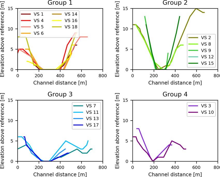
P. Hulsman et al.: Altimetry for model calibration                                                                        3333

modelled discharge arising from the missing information           the annual basin water balance (World Bank, 2010). The
on flow amounts, data from the Gravity Recovery and Cli-          landscape varies between low-lying flat areas along the river
mate Experiment (GRACE), which provides estimates of the          to large escarpments mostly in the north-west of the basin
monthly total water storage anomalies, were used to sup-          and highlands with an elevation difference of up to 1850 m
port model calibration. With GRACE, discharge can be con-         (see Fig. 1b and Sect. 3.2 for more information on the land-
strained through improved simulation of the rainfall parti-       scape classification). During the dry season, the river mean-
tioning into runoff and evaporation as illustrated in previous    ders between sandy banks, while during the wet season from
studies (Rakovec et al., 2016; Bai et al., 2018).                 November to May it can cover floodplains several kilometres
   Therefore, the overarching objective of this study is to ex-   wide.
plore the combined information content (cf. Beven, 2008)             The Luangwa drains into the Zambezi downstream of the
of river altimetry data from multiple satellite missions and      Kariba Dam and upstream of the Cahora Bassa Dam. The
GRACE observations to identify feasible parameter sets for        operation of both dams is crucial for hydropower production
the calibration of hydrological models of large river systems     and flood and drought protection, but is very difficult due to
in a semi-arid, data-scarce region.                               the lack of information from poorly gauged tributaries such
   More specifically, in a step-wise approach we use GRACE        as the Luangwa (SADC-WD and Zambezi River Authority,
observations together with altimetry data from multiple vir-      2008; Schleiss and Matos, 2016; World Bank, 2010). As a re-
tual stations to identify model parameters following three        sult, the local population has suffered from severe floods and
different strategies, and we compare model performances to        droughts (ZAMCOM et al., 2015; Beilfuss and dos Santos,
a traditional calibration approach based on in situ observed      2001; Hanlon, 2001; SADC-WD and Zambezi River Author-
river discharge. These three strategies compare altimetry ob-     ity, 2008; Schumann et al., 2016).
servations to (1) modelled discharge by applying the Spear-
man rank correlation coefficient and to modelled stream lev-      2.1     Data availability
els by converting modelled discharge using (2) rating curves
whose parameters were treated as free model calibration pa-       2.1.1    In situ discharge and water-level observations
rameters and (3) the Strickler–Manning equation to infer
water levels directly from hydraulic properties of the river.     In the Luangwa basin, historical in situ daily discharge and
These three strategies are tested on a distributed process-       water-level observations were available from the Zambian
based rainfall–runoff model with sub-grid process hetero-         Water Resources Management Authority (WARMA) at the
geneity for the Luangwa basin. More specifically, we test         Great East Road Bridge gauging station, located at 30◦ 130 E
the following research hypotheses: (1) the use of altimetry       and 14◦ 580 S (Fig. 1) about 75 km upstream of the confluence
data combined with GRACE observations allows a meaning-           with the Zambezi. In this study, all complete hydrological
ful selection of feasible model parameter sets to reproduce       years of discharge data within the time period 2002 to 2016
river discharge depending on the applied parameter identifi-      were used; these are the years 2004, 2006, and 2008.
cation strategy, and (2) the combined application of multiple
virtual stations from multiple satellite missions improves the    2.1.2    Gridded data products
model’s ability to reproduce observed hydrological dynam-
ics.                                                              Besides the in situ observations, gridded data products were
                                                                  used in this study for topographic description, model forcing
                                                                  (precipitation and temperature), and model parameter selec-
2   Site description                                              tion/calibration (total water storage anomalies), as shown in
                                                                  Table 1. The temperature data were used to estimate the po-
The study area is the Luangwa River in Zambia, a tribu-           tential evaporation according to the Hargreaves method (Har-
tary of the Zambezi River (Fig. 1). It has a basin area of        greaves and Samani, 1985; Hargreaves and Allen, 2003).
159 000 km2 , which is about 10 % of the Zambezi River               Gravity Recovery and Climate Experiment (GRACE) ob-
basin. The Luangwa basin is poorly gauged, mostly unreg-          servations describe monthly total water storage anomalies
ulated, and sparsely populated with about 1.8 million in-         which include all terrestrial water stores present in the
habitants in 2005 (World Bank, 2010). The mean annual             groundwater, soil moisture, and surface water. Two identical
precipitation is around 970 mm yr−1 , potential evaporation       satellites observe the variations in the Earth’s gravity field
is around 1555 mm yr−1 , and river runoff reaches about           to detect regional mass changes which are dominated by
100 mm yr−1 (World Bank, 2010). The main land cover con-          variations in the terrestrial water storage once atmospheric
sists of broadleaf deciduous forest (55 %), shrubland (25 %),     effects have been accounted for (Landerer and Swenson,
and savanna grassland (16 %) (ESA and UCLouvian, 2010).           2012; Swenson, 2012). In this study, processed GRACE ob-
The irrigated area in the basin is limited to about 180 km2 ,     servations of Release 05 generated by the CSR (Centre for
i.e. roughly 0.1 % of the basin area with an annual water         Space Research), GFZ (GeoForschungsZentrum Potsdam),
use of about 0.7 mm yr−1 , which amounts to < 0.001 % of          and JPL (Jet Propulsion Laboratory) were downloaded from

https://doi.org/10.5194/hess-24-3331-2020                                       Hydrol. Earth Syst. Sci., 24, 3331–3359, 2020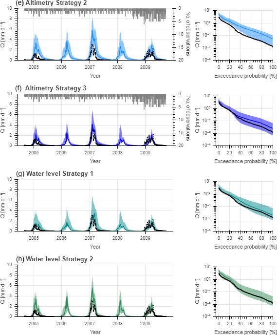
3334 P. Hulsman et al.: Altimetry for model calibration
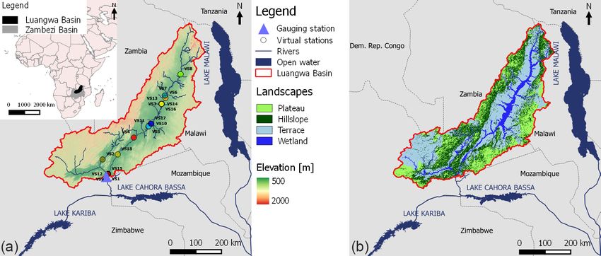
Figure 1. (a) Elevation map of the Luangwa River basin in Zambia including the Great East Road Bridges river gauging station and the
locations of the 18 virtual stations (VS 1–VS 18; the red dot is VS 4) with altimetry data used in this study; their colours correspond to those
in Fig. 4. (b) Map of the Luangwa River basin with the main landscape types (see Sect. 3.2).
Table 1. Gridded data products used in this study.
Time period Time resolution Spatial resolution Product name Source
Digital elevation map n/a n/a 0.02◦ GMTED (Danielson and Gesch, 2011)
Precipitation 2002–2016 Daily 0.05◦ CHIRPS (Funk et al., 2014)
Temperature 2002–2016 Monthly 0.5◦ CRU (University of East Anglia Climatic
Research Unit et al., 2017)
Total water storage 2002–2016 Monthly 1◦ GRACE (Swenson, 2012; Swenson and Wahr,
2006; Landerer and Swenson, 2012)
n/a means not applicable.
the GRACE Tellus website (https://grace.jpl.nasa.gov/, last 2.1.3 Altimetry data
access: June 2017). The averages of all three sources were
used. The raw data were previously processed by the CSR, The altimetry data used in this study were obtained
GFZ, and JPL to remove atmospheric mass changes us- from the following sources: the Database for Hydrologi-
ing ECMWF (European Centre for Medium-Range Weather cal Time Series of Inland Waters (DAHITI; https://dahiti.
Forecasts) atmospheric pressure fields, systematic errors dgfi.tum.de/en/, last access: February 2018) (Schwatke
causing north–south-oriented stripes, and high-frequency et al., 2015), HydroSat (http://hydrosat.gis.uni-stuttgart.de/
noise using a 300 km wide Gaussian filter via spatial smooth- php/index.php, last access: February 2018) (Tourian et al.,
ing (Swenson and Wahr, 2006; Landerer and Swenson, 2012; 2013), Laboratoire d’Etudes en Géophysique et Océanogra-
Wahr et al., 1998). Processed GRACE observations de- phie Spatiales (LEGOS; http://www.legos.obs-mip.fr/soa/
scribe terrestrial water storage anomalies in “equivalent wa- hydrologie/hydroweb/, last access: March 2018; see supple-
ter thickness” in centimetres relative to the 2004–2009 time- ments for more information), and the Earth and Planetary
mean baseline. In other words, the water storage anomaly is Remote Sensing Lab (EAPRS; http://www.cse.dmu.ac.uk/
the water storage minus the long-term mean (Landerer and EAPRS/, last access: February 2018). In total, altimetry data
Swenson, 2012). were obtained for 18 virtual stations in the Luangwa basin
All gridded information was rescaled to the model resolu- (Fig. 1a) for the time period 2002–2016 from satellite mis-
tion of 0.1◦ . The temperature and GRACE data were rescaled sions Jason 1–3, Envisat, and Saral (Table 2, Fig. S2).
by dividing each cell of the satellite product into multiple
cells such that the model resolution is obtained, retaining the 2.1.4 River geometry information
original value. The precipitation was rescaled by taking the
average of all cells located within each model cell. In the Luangwa basin, very limited detailed in situ informa-
tion was available on the river geometry such as cross sec-
Hydrol. Earth Syst. Sci., 24, 3331–3359, 2020 https://doi.org/10.5194/hess-24-3331-2020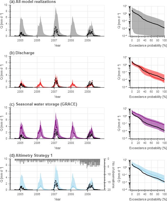
Table 2. Overview of the altimetry data in the Luangwa River basin used in this study.

                                                 Nr.    Longitude       Latitude    Time period     Nr. of days    Source       Mission          Space Agency   Temporal     Equatorial   Along-       Literature
                                                                                                    with data                                                   resolution   inter-       track
                                                                                                                                                                             track        distance
                                                                                                                                                                             distance
                                                 1       30.2823◦    −14.8664◦      2008–2016               246    DAHITI       Jason 2, 3       NASA/CNES      10 d         315 km       294 m        (Schwatke et al.,
                                                                                                                                                                                                       2015; CNES,
                                                                                                                                                                                                       Accessed 2018)
                                                 2       30.0864◦      −14.366◦     2008–2015                92    DAHITI       Jason 2, 3
                                                 3       32.1715◦    −12.4123◦      2008–2016               248    DAHITI       Jason 2, 3
                                                 4       31.1868◦    −13.5927◦      2002–2016               104    DAHITI       Envisat, Saral   ESA            35 d         80 km        374 m        (Schwatke et al.,
                                                                                                                                                 (Envisat),                  (Envisat),   (Envisat),   2015; ESA, 2018;

https://doi.org/10.5194/hess-24-3331-2020
                                                                                                                                                 ISRO/CNES                   75 km        173 m        CNES, Accessed
                                                                                                                                                 (Saral)                     (Saral)      (Saral)      2018)
                                                 5       31.6984◦    −13.2039◦      2002–2016                82    DAHITI       Envisat, Saral
                                                                                                                                                                                                                            P. Hulsman et al.: Altimetry for model calibration

                                                 6       32.2998◦    −12.2007◦      2002–2016               100    DAHITI       Envisat, Saral
                                                 7       32.2805◦    −12.1157◦      2002–2016               103    DAHITI       Envisat, Saral
                                                 8        32.831◦    −11.3674◦      2002–2016               105    DAHITI       Envisat, Saral
                                                 9       30.2704◦    −14.8809◦      2008–2015               247    HydroSat     Jason 2          NASA/CNES      10 d         315 km       294 m        (Tourian et al.,
                                                                                                                                                                                                       2016; Tourian
                                                                                                                                                                                                       et al., 2013)
                                                 10     31.78405◦    −13.0995◦      2002–2010                65    EAPRS        Envisat          ESA            35 d         80 km        374 m        (Michailovsky
                                                                                                                                                                                                       et al., 2012; ESA,
                                                                                                                                                                                                       2018)
                                                 11     31.71099◦    −13.1943◦      2002–2010                93    EAPRS        Envisat
                                                 12      30.2740◦    −14.8763◦      2008–2015               231    LEGOS        Jason 3          NASA/CNES      10 d         315 km       294 m        (Frappart et al.,
                                                                                                                                                                                                       2015; CNES,
                                                                                                                                                                                                       Accessed 2018)
                                                 13     32.15843◦      −12.412◦     2016–2016                28    LEGOS        Jason 3
                                                 14     32.15989◦    −12.4127◦      2002–2009               137    LEGOS        Jason 1
                                                 15      30.2740◦    −14.8763◦      2008–2016               271    LEGOS        Jason 2
                                                 16     32.16056◦    −12.4125◦      2008–2016               283    LEGOS        Jason 2
                                                 17     31.80001◦    −13.0909◦      2013–2016                35    LEGOS        Saral            ISRO/CNES      35 d         75 km        173 m
                                                 18     30.61577◦    −14.1852◦      2013–2016                24    LEGOS        Saral

Hydrol. Earth Syst. Sci., 24, 3331–3359, 2020
                                                                                                                                                                                                                            3335
3336 P. Hulsman et al.: Altimetry for model calibration
tion and slope. For that reason, this information was extracted water levels using the Strickler–Manning equation and in-
from global high-resolution terrain data available on Google cluding river geometry information (cross section and gra-
Earth (2018) as done successfully in previous studies for dient) extracted from Google Earth combined with GRACE
other purposes (Pandya et al., 2017; Zhou and Wang, 2015). data; (4a) Water level Strategy 1: identification of parameter
This was done for each virtual station and the basin out- sets based on daily river water level at the catchment out-
let. Google Earth only provides river geometry information let only using the Strickler–Manning equation and includ-
above the river water level. As the Luangwa is a perennial ing river geometry information extracted from Google Earth
river, parts of the cross section remain submerged through- combined with GRACE data; and (4b) Water level Strat-
out the year and are thus unknown. To limit uncertainties egy 2: identification of parameter sets based on daily river
arising from this issue, the cross-section geometry for each water level at the catchment outlet only using the Strickler–
virtual station was extracted from Google Earth images with Manning equation and including river geometry information
the lowest water levels. The dates of these images in gen- obtained from a detailed field survey with an ADCP com-
eral fall in the dry season, with flows at the Great East Road bined with GRACE data. Note that (1) is completely inde-
Bridges gauging station on the respective days ranging from pendent of (2) to (4), where no discharge data were used for
1 % to 4 % relative to the maximum discharge (see Table S3 the identification of parameter sets.
in the Supplement for the dates of the satellite images and the
associated flows at the Great East Road Bridges gauging sta- 3.2 Hydrological model structure
tion). The database underlying the global terrain images in
Google Earth originate from multiple, merged data sources In this study, a process-based rainfall–runoff model with dis-
with varying spatial resolutions. For the Luangwa basin these tributed water accounting and sub-grid process heterogeneity
include the Shuttle Radar Topography Mission (SRTM) with was developed (Ajami et al., 2004; Euser et al., 2015). The
a spatial resolution of 30 m, Landsat 8 with a spatial resolu- river basin was discretized into a grid with a spatial resolu-
tion of 15 m, and the Satellite Pour l’Observation de la Terre tion of 10 × 10 km2 . Each model grid cell was characterized
4/5 (SPOT) with a spatial resolution of 2.5 to 20 m (Smith by the same model structure and parameter sets but forced
and Sandwell, 2003; Irons et al., 2012; Drusch et al., 2012). by spatially distributed, gridded input data (Table 1). Runoff
In addition to Google Earth data, the submerged part of the was then calculated in parallel for each cell separately. Sub-
channel cross section was surveyed in the field on 27 April sequently, a routing scheme was applied to estimate the ag-
2018 near the Great East Road Bridges river gauging station gregated flow in each grid cell at each time step.
at the coordinates 30◦ 130 E and 15◦ 000 S (Abas, 2018) with Adopting the FLEX-Topo modelling concept (Savenije,
an Acoustic Doppler Current Profiler (ADCP). 2010) and extending it to a gridded implementation, each
grid cell was further discretized into functionally distinct hy-
drological response units (HRUs) as demonstrated by Ni-
3 Hydrological model development jzink et al. (2016). Each point within a grid cell was as-
signed to a response class based on its position in the land-
3.1 General approach scape as defined by its local slope and “Height-above-the-
nearest-drainage” (HAND; Rennó et al., 2008; Gharari et al.,
The potential of river altimetry for model calibration was 2011). Similarly to previous studies (e.g. Gao et al., 2016;
tested with a process-based hydrological model for the Lu- Nijzink et al., 2016), the response units plateau, hillslope, ter-
angwa River basin. This model relied on distributed forcing race, and wetland were distinguished. Reflecting earlier work
allowing for spatially explicit distributed water storage cal- (e.g. Gharari et al., 2011), all locations with a slope of > 4 %
culations. The model was run on a daily timescale for the were assumed to be hillslope. Locations with lower slopes
time period 2002 to 2016. To reach the objective of this study, were then either defined as wetland (HAND < 11 m), ter-
the following distinct parameter identification strategies were race (11 m ≤ HAND < 275 m), or plateau (HAND ≥ 275 m);
compared in a step-wise approach: (1) traditional model cal- see Fig. 2. Following this classification, wetlands make
ibration to observed river flow as a benchmark; (2) iden- up pHRU = 8 %, terraces pHRU = 41 %, hillslopes pHRU =
tification of parameter sets reproducing the seasonal water 28 %, and plateaus pHRU = 23 % of the total Luangwa River
storage anomalies based on GRACE data only; (3a) Altime- basin area as mapped in Fig. 1b.
try Strategy 1: identification of parameter sets directly based Each response class consisted of a series of storage com-
on remotely sensed water levels combined with GRACE ponents that were linked by fluxes. The flow generated from
data; (3b) Altimetry Strategy 2: identification of parameter each grid cell at any given time step was then computed as
sets based on remotely sensed water levels by converting the area-weighted flow from the individual response units
modelled discharges into water levels using calibrated rating plus a contribution from the common groundwater compo-
curves combined with GRACE data; (3c) Altimetry Strat- nent which connects the response units (Fig. 2). Finally, the
egy 3: identification of parameter sets based on remotely outflow from each modelling cell was routed to downstream
sensed water levels by converting modelled discharges into cells to obtain the accumulated flow in each grid cell at any
Hydrol. Earth Syst. Sci., 24, 3331–3359, 2020 https://doi.org/10.5194/hess-24-3331-2020P. Hulsman et al.: Altimetry for model calibration 3337
Figure 2. Sketch of the hydrological response units including the thresholds used in this analysis for the slope and HAND (height above
nearest drainage) and including their corresponding model structures. This spatial sub-grid discretization was applied to each grid cell.
Symbol explanation: precipitation (P ), effective precipitation (Pe ), interception evaporation (Ei ), plant transpiration (Et ), infiltration into the
unsaturated root zone (Ru ), drainage to the fast runoff component (Rf ), delayed fast runoff (Rfl ), lag time (Tlag ), groundwater recharge (Rr ),
upwelling groundwater flux (RGW ), fast runoff (Qf ), groundwater/slow runoff (Qs ).
given time step. For this purpose, the mean flow length of Jakeman and Hornberger, 1993). Thus, to reduce the risk of
each model grid cell to the outlet was derived based on the rejecting good parameters when they should have been ac-
flow direction extracted from the digital elevation model. The cepted (Beven, 2010; Hrachowitz and Clark, 2017), we rather
flow velocity, which was assumed to be constant in space attempted to identify and discard the most implausible pa-
and time, was calibrated. With this information on the flow rameter sets (Freer et al., 1996) that violate our theoretical
path length and velocity, the accumulated flow in each grid understanding of the system or that are inconsistent with the
cell was calculated at the end of each time step. The relevant available data (Knutti, 2008). This allowed us to iteratively
model equations are given in Table 3. This concept was pre- constrain the feasible parameter space and thus the uncer-
viously successfully applied in a wide range of environments tainty around the modelled hydrograph (Hrachowitz et al.,
(Gao et al., 2014; Gharari et al., 2014; Fovet et al., 2015; 2014). To do so, a Monte Carlo sampling strategy with uni-
Nijzink et al., 2016; Prenner et al., 2018). form prior parameter distributions was applied to generate
5 × 10⁴ model realizations. This random set of solutions was
3.3 Parameter selection procedures in the following steps used as a baseline and iteratively con-
strained by identifying parameter sets that do not satisfy pre-
To evaluate the information content and thus the utility of specified criteria (see below), depending on the data type and
altimetry data for the selection of feasible model parame- source used.
ter sets, a step-wise procedure as specified in detail below
was applied (Table 5). Note that given data scarcity and the
3.3.1 Benchmark: parameter selection based on
related issues of epistemic uncertainties (Beven and Wester-
observed discharge data
berg, 2011; McMillan and Westerberg, 2015) and equifinal-
ity (Beven, 2006; Savenije, 2001) we did not aim to iden-
tify the “optimal” parameter set in what is frequently con- As a benchmark, and following a traditional calibration pro-
sidered a traditional calibration approach. In most hydrolog- cedure, the model was calibrated with observed daily dis-
ical applications the available data have limited strength for charge based on the Nash–Sutcliffe efficiency (ENS,Q , Eq. 1)
rigorous model tests (Clark et al., 2015; Gupta et al., 2008; in Table 4 using all complete hydrological years within the
https://doi.org/10.5194/hess-24-3331-2020 Hydrol. Earth Syst. Sci., 24, 3331–3359, 20203338 P. Hulsman et al.: Altimetry for model calibration
Table 3. Equations applied in the hydrological model. Fluxes (mm d−1 ): precipitation (P ), effective precipitation (Pe ), potential evaporation
(Ep ), interception evaporation (Ei ), plant transpiration (Et ), infiltration into the unsaturated zone (Ru ), drainage to fast runoff component
(Rf ), delayed fast runoff (Rfl ), groundwater recharge (Rr for each relevant HRU and Rr,tot combining all relevant HRUs), upwelling ground-
water (RGW for each relevant HRU and RGW,tot combining all relevant HRUs), fast runoff (Qf for each HRU and Qf,tot combining all
HRUs), groundwater/slow runoff (Qs ), total runoff (Qm ). Storages (mm): storage in interception reservoir (Si ), storage in unsaturated root
zone (Su ), storage in groundwater/slow reservoir (Ss ), storage in fast reservoir (Sf ). Parameters: interception capacity (Imax ) (mm), maxi-
mum upwelling groundwater (Cmax ) (mm d−1 ), maximum root zone storage capacity (Sumax ) (mm), splitter (W ) (–), shape parameter (β)
(–), transpiration coefficient (Ce ) (–), time lag (Tlag ) (d), reservoir timescales (d) of fast (Kf ) and slow (Ks ) reservoirs, areal weights (pHRU )
(–), time step (1t) (d). Model parameters are shown in bold letters in the table below. The equations were applied to each hydrological
response unit (HRU) unless indicated differently.
Reservoir system Water balance equation Process functions
1Si
Interception 1t = P − Pe − Ei ≈ 0 Ei = min Ep , min P , I1t
max
Pe = P − Ei
Su
, Ep − Ei · S Su · C1 )
Unsaturated zone Plateau/terrace: Et = min( Ep − Ei min 1t
1Su u,max e
1t = Pe − Et − Rf Ss
Su 1t
Hillslope: RGW = min 1 − S · Cmax , pHRU
u,max
1Su
1t = Ru − Et if Su + RGW · 1t > Su,max : RGW =
Su,max −Su
Wetland: 1t
1Su Hillslope:
1t = Pe − Et − Rf + RGW Ru = (1 − C) · Pe
β
C = 1 − 1 − S Su
u,max
1Sf Sf
Fast runoff 1t = Rfl − Qf Qf = K
f
Plateau/terrace/wetland:
Rf = max(0, S1t
u −Sumax )
Rfl = Rf
Hillslope:
Rf = (1 − W ) · C · Pe
Rfl = Rf ∗f (Tlag )
1Ss
Groundwater 1t = Rrtot − RGWtot − Qs Rr = W P · C · Pe
Rrtot = pHRU · Rr
HRUP
RGWtot = pHRU · RGW
HRU
Ss
Qs = K
s
P
Total runoff Qm = Qs + Qftot Qftot = pHRU · Qf
HRU
Supporting literature Gharari et al. (2014); Gao et al. (2014); Euser et al. (2015)
time period 2002 to 2016 (Nash and Sutcliffe, 1970). These 3.3.2 Parameter selection based on the seasonal water
are the years starting in the fall of 2004, 2006, and 2008. storage (GRACE)
To limit the solutions to relatively robust representations
of the system while allowing for data and model uncertainty In a next step we assumed that discharge records in the Lu-
(e.g. Beven, 2006; Beven and Westerberg, 2011), only pa- angwa basin were absent. The starting assumption thus had to
rameter sets that resulted in ENS,Q ≥ 0.6 were retained as be that all model realizations, i.e. all sampled parameter sets,
feasible. The hydrological model consisted of 18 free calibra- were equally likely to allow feasible representations of the
tion parameters (Table 5, Fig. S1 in the Supplement) whose hydrological system. In a step-wise approach, confronting
uniform prior distributions are given in Table S1 in the Sup- these realizations with different types of data, we sequen-
plement with associated parameter constraints as summa- tially identified and discarded solutions that were least likely
rized in Table S2. to provide meaningful system representations, thereby grad-
ually narrowing down the feasible parameter space.
We first identified and discarded solutions that were least
likely to preserve observed seasonal water storage (Stot ) fluc-
Hydrol. Earth Syst. Sci., 24, 3331–3359, 2020 https://doi.org/10.5194/hess-24-3331-2020P. Hulsman et al.: Altimetry for model calibration 3339
Table 4. Equations used to calculate the model performance.
Name Objective function Symbol explanation Equation no.
(θmod (t) − θobs (t))2
P
t
Nash–Sutcliffe ENS,θ = 1 − P θ : variable (1)
¯ 2
θobs (t) − θobs
t
cov(rQ,mod , rWL,obs )
Spearman rank cor- ER,WL = rQ,mod : ranks of the modelled (2)
relation σ rQ,mod · σ (rWL,obs ) discharge
coefficient rWL,obs : ranks of the observed
water levels
|θmod − θobs |
Relative error ER,θ = 1 − θ : variable (3)
θobs
v !
u
u P 2
Euclidian distance DE,β,γ = 1 − t wi · 1 − Eβ,γ wi : relative weight of virtual (4)
over multiple i station i
virtual stations β: model performance metric
γ : parameter selection method
v !
u
u 1 X 2 X 2
Euclidian distance DE = 1−t 1 − ENS,θn + 1 − ER,θm θ : signature (5)
(N + M) n m
over multiple n: signatures evaluated with
signatures Eq. (1) with maximum N
m: signatures evaluated with
Eq. (3) with maximum M
tuations. To do so, the monthly modelled total water stor- no time series of river flow available), we kept for each strat-
age (Stot,mod = Si + Su + Sf + Ss ) relative to the 2004–2009 egy as feasible the respective 1 % best performing parameter
time-mean baseline in each grid cell was compared to water sets according to the specific performance metric associated
storage anomalies observed with GRACE where this same with that strategy.
time-mean baseline was used (Tang et al., 2017; Fang et al.,
2016; Forootan et al., 2019; Khaki and Awange, 2019). Altimetry Strategy 1: direct comparison of altimetry
The model’s skill at reproducing the seasonal water stor- data to modelled discharge
age, i.e. Stot , was assessed using the Nash–Sutcliffe effi-
ciency ENS,Stot (Eq. 1). Note that ENS,Stot,j was computed In the simplest approach, we directly used altimetry data
at first from the time series of Stot in each grid cell j which to correlate observed water levels with modelled discharge
were then averaged to obtain ENS,Stot . If no additional data based on the Spearman rank correlation coefficient (ER,WL ;
were available, a hypothetic modeller relying on ENS,Stot to Spearman, 1904) using Eq. (2) (Table 4). This strategy, here-
calibrate a model may choose only the solution with the high- after referred to with subscript WL, i.e. water level, re-
est ENS,Stot or allow for some uncertainty. To mimic this tra- quires the assumption that the relationship between water
ditional approach and balance it with a sufficient number of level and discharge is monotonic. The Spearman rank cor-
feasible solutions to be kept for the subsequent steps, we here relation was applied successfully in previous studies to cali-
identified and discarded the poorest performing 75 % of all brate a rainfall–runoff model to water-level time series (Seib-
solutions in terms of ENS,Stot as unfeasible for the subsequent ert and Vis, 2016). As there were multiple virtual stations
modelling steps. with water-level data available in this study, the ER,WL was
computed at each location simultaneously. The individual
3.3.3 Parameter selection based on satellite altimetry values ER,WL were weighted based on the record length of
data the corresponding virtual stations and then combined into the
Euclidean distance as aggregate metric DE,R,WL with Eq. (4).
Next, the remaining feasible parameter sets were used to
evaluate their potential to reproduce time series of observed
altimetry applying three distinct parameter selection strate-
gies. Assuming again the situation of an ungauged basin (i.e.
https://doi.org/10.5194/hess-24-3331-2020 Hydrol. Earth Syst. Sci., 24, 3331–3359, 2020P. Hulsman et al.: Altimetry for model calibration
https://doi.org/10.5194/hess-24-3331-2020
Table 5. Overview of the parameter identification strategies applied in this study.
Strategy Calibration data Objective function Parameter group Calibration parameters Comments Q–h conversion Benefits (+) & limitations (−)
Discharge Discharge ENS,Q (Eq. 1) Entire basin Ks , Ce Traditional model calibration − −
(reference) (at basin outlet) Plateau & Terrace Imax , Sumax , Kf , W on observed flow data
Hillslope Imax , Sumax , Kf , W , β, Tlag Combination of 8 different flow
Wetland Imax , Sumax , Kf , W , Cmax signatures
River profile v
Total: 18
Seasonal GRACE ENS,Stot (Eq. 1) Entire basin Ks , Ce No discharge data used − −
water Plateau & Terrace Imax , Sumax , Kf , W
storage Hillslope Imax , Sumax , Kf , W , β, Tlag
Wetland Imax , Sumax , Kf , W , Cmax
River profile v
Total: 18
Altimetry Altimetry Altimetry: DE,R,WL Entire basin Ks , Ce No discharge data used − + No extra parameters or data needed
Strategy 1 (at 18 virtual (Eqs. 2 and 4) Plateau & Terrace Imax , Sumax , Kf , W Combination of 18 virtual + Assumption: monotonic relation between
stations) GRACE: ENS,Stot Hillslope Imax , Sumax , Kf , W , β, Tlag stations discharge and river water level
& GRACE (Eq. 1) Wetland Imax , Sumax , Kf , W , Cmax Combined with GRACE − Focus on dynamics only, not volume
River profile v
Total: 18
Altimetry Altimetry Altimetry: DE,NS,RC Entire basin Ks , Ce No discharge data used CalibratedRating curve + No extra data needed
Strategy 2 (at 18 virtual (Eqs. 1 and 4) Plateau & Terrace Imax , Sumax , Kf , W Combination of 18 virtual − Two extra parameters per cross section
stations) GRACE: ENS,Stot Hillslope Imax , Sumax , Kf , W , β, Tlag stations
& GRACE (Eq. 1) Wetland Imax , Sumax , Kf , W , Cmax Combined with GRACE
River profile v, a1 , a2 , a3 , a4 , b1 , b2 , b3 , b4
Total: 26
Altimetry Altimetry Altimetry: DE,NS,SM Entire basin Ks , Ce No discharge data used Strickler–Manning + Only 1 extra parameter
Strategy 3 (at 18 virtual (Eqs. 1 and 4) Plateau & Terrace Imax , Sumax , Kf , W Combination of 18 virtual − Cross-section data needed
Hydrol. Earth Syst. Sci., 24, 3331–3359, 2020
stations) GRACE: ENS,Stot Hillslope Imax , Sumax , Kf , W , β, Tlag stations − Assumption: constant roughness in space
& GRACE (Eq. 1) Wetland Imax , Sumax , Kf , W , Cmax Combined with GRACE and time
River profile v, k
Total: 18
Water level Water level Altimetry: ENS,SM,GE Entire basin Ks , Ce No discharge data used Strickler–Manning + Only 1 extra parameter
Strategy 1 (at basin outlet) (Eq. 1) Plateau & Terrace Imax , Sumax , Kf , W Combined with GRACE − Cross-section data needed
& GRACE GRACE: ENS,Stot Hillslope Imax , Sumax , Kf , W , β, Tlag − Assumption: constant roughness in space
(Eq. 1) Wetland Imax , Sumax , Kf , W , Cmax and time
River profile v, k
Total: 19
Water level Water level Altimetry: Entire basin Ks , Ce No discharge data used Strickler–Manning + Only 1 extra parameter
Strategy 2 (at basin outlet) ENS,SM,ADCP (Eq. 1) Plateau & Terrace Imax , Sumax , Kf , W Combined with GRACE − Cross-section data needed
& GRACE GRACE: ENS,Stot Hillslope Imax , Sumax , Kf , W , β, Tlag − Assumption: constant roughness in space
(Eq. 1) Wetland Imax , Sumax , Kf , W , Cmax and time
River profile v, k
Total: 19
3340P. Hulsman et al.: Altimetry for model calibration 3341
Altimetry Strategy 2: rating curves
1 2
In the second strategy, as successfully applied in previous A = B ·d + · d · (i1 + i2 ) , (8)
2
studies (Getirana and Peters-Lidard, 2013; Jian et al., 2017), A
model parameters were selected based on the models’ abil- R= , (9)
2
21 2
12
ity to reproduce water levels by converting the modelled B + d · 1 + i1 + 1 + i2
discharge to water levels, assuming these two are related
through a rating curve in the form of a power function (Rantz, d = h − h0 , (10)
1982):
where B is the assumed river bed width, i1 and i2 are the
b
Q = a · (h − h0 ) , (6) river bank slopes, d is the water depth, h is the water level,
and h0 is the reference water level, here assumed to be the
where h is the water level, h0 is a reference water level, and lowest observed river water level to limit the number of cal-
a and b are two additional free calibration parameters deter- ibration parameters. In contrast to previous studies that use
mining the shape of the function and lumping combined in- a similar approach but relied on locally observed river cross
fluences of different river cross-section characteristics such sections (Michailovsky et al., 2012; Hulsman et al., 2018;
as geometry or roughness. Note that here for each virtual sta- Liu et al., 2015), here both the river bed geometries (Fig. 3)
tion h0 is the elevation that corresponds to the water level of at and the channel slopes upstream of the 18 virtual stations
the Google Earth image with the lowest flow available, cor- were computed using high-resolution terrain data retrieved
responding to the assumption of no-flow at that time. This from Google Earth (see Sect. 2.1.4). Similar data sources
strategy is hereafter referred to with subscript RC, i.e. rat- were already used in previous studies to extract the river ge-
ing curve. As river cross sections vary in space, each of the ometry (e.g. Michailovsky et al., 2012; Pramanik et al., 2010;
18 virtual stations would require an individual set of these Gichamo et al., 2012). The reader is referred to Table S3 for
parameters a and b. To limit the number of additional cali- the values of the variables for each virtual station. This strat-
bration parameters, we here classified the river cross sections egy is hereafter referred to with subscript SM, i.e. Strickler–
of the 18 virtual stations into four groups (Figs. 1a and 3). For Manning.
cross sections within each class, i.e. geometrically similar, Equivalent to above, the modelled river water levels were
the same values for a and b were used, resulting in four sets then evaluated against the observed water levels at each
of a and b and thus a total of eight additional calibration pa- virtual station using the Nash–Sutcliffe efficiency ENS,SM
rameters. The river cross sections were extracted from global (equivalent to Eq. 1), weighted based on the record length of
high-resolution terrain data available on Google Earth (see the corresponding virtual stations and then combined into the
Sect. 2.1.4). The modelled river water levels were evalu- Euclidean distance DE,NS,SM as an aggregated performance
ated against the observed water levels at each virtual sta- metric (Eq. 4).
tion using the Nash–Sutcliffe efficiency ENS,RC (equivalent
to Eq. 1 in Table 4), weighted based on the record length of 3.3.4 Parameter selection based on daily river water
the corresponding virtual stations and then combined into the level at the basin outlet
Euclidean distance DE,NS,RC as an aggregated performance
For the previous parameter identification strategy (Altimetry
metric (Eq. 4).
Strategy 3), river geometry information was extracted from
Altimetry Strategy 3: Strickler–Manning equation high-resolution terrain data retrieved from Google Earth,
which have a low accuracy. Unfortunately, more accurate
As a third strategy, we converted the modelled discharge cross-section information from in situ surveys was only
to river water levels using the Strickler–Manning equation available at the Great East Road Bridge gauging station, i.e.
(Manning, 1891): the basin outlet, where, in turn, no altimetry observations
were available. That is why water-level time series were used
1 2
Q = k·i2 ·A·R3, (7) to illustrate the influence of the cross-section accuracy.
As shown in Fig. 5, the Google Earth based above-water
where k is a roughness parameter here treated as a free cal- cross section at the basin outlet corresponded in general well
ibration parameter and assumed constant for all virtual sta- to the field survey considering that satellite images have lim-
tions, i is the mean channel slope extracted here over a dis- ited spatial resolution. However, the in situ measurement also
tance of 10 km, and A and R are the river cross-section area illustrated the relevance of the submerged part of the channel
and hydraulic radius. Assuming trapezoidal cross sections cross section at that location on the day the image was taken
(see Fig. 4 as an illustrative example), A and R were cal- (2 June 2008).
culated for each cross section according to
https://doi.org/10.5194/hess-24-3331-2020 Hydrol. Earth Syst. Sci., 24, 3331–3359, 20203342 P. Hulsman et al.: Altimetry for model calibration
Figure 3. River profiles at 18 virtual stations (VS) divided into four groups. The reference level is equal to the lowest water level in the river
profile for each location separately.
Figure 4. Example of approximating a trapezoidal cross section
(black) into the Google Earth based cross-section data (red) for vir-
tual station “VS 4” (see also Fig. 1a and Fig. 3). The reference level
is equal to the lowest water level in the river profile.
Figure 5. River cross section at Luangwa Bridge obtained from
Water level Strategy 1: river geometry information Google Earth and detailed field survey including the river water
extracted from Google Earth level on 2 June 2008. Field measurements were done with an Acous-
tic Doppler Current Profiler (ADCP) on 27 April 2018 at the coordi-
nates 30◦ 130 E and 15◦ 000 S; the satellite image was taken on 2 June
First, cross-section information was extracted from global 2008. The reference level is equal to the lowest elevation level mea-
high-resolution terrain data available on Google Earth (sub- sured with the ADCP.
script GE) and used with the Strickler–Manning equation
(Eq. 7) to convert the modelled discharge to water levels.
This was combined with GRACE observations to restrict the
parameter space in an equivalent way to Sect. 3.3.3. The
Hydrol. Earth Syst. Sci., 24, 3331–3359, 2020 https://doi.org/10.5194/hess-24-3331-2020P. Hulsman et al.: Altimetry for model calibration 3343
model performance with respect to river water levels was cal- Fig. 7 and tabulated in Table S4. Although containing rela-
culated with the Nash–Sutcliffe efficiency ENS,SM,GE (Eq. 1). tively good solutions, this full set of all realizations clearly
also contained many parameter sets that considerably over-
Water level Strategy 2: river geometry information estimated and/or underestimated flows.
obtained from a detailed field survey
4.1.1 Benchmark: parameter selection based on
Second, cross-section information obtained from a detailed observed discharge data
field survey with an ADCP (subscript ADCP) was used with
the Strickler–Manning equation (Eq. 7) to convert the mod- For the benchmark case, applying the traditional model cali-
elled discharge to water levels. This was combined with bration approach using discharge data, this parameter selec-
GRACE observations to restrict the parameter space in an tion and calibration strategy resulted in a reasonable model
equivalent way to Sect. 3.3.3. The model performance with performance, in which the seasonal but also the daily flow
respect to river water levels was calculated with the Nash– dynamics and magnitudes were in general well captured
Sutcliffe efficiency ENS,SM,ADCP (Eq. 1). as shown in Fig. 6b. For some years, a number of solu-
tions overestimated flows in the wet season and underesti-
3.4 Model evaluation mated flows during the dry season, when the river becomes
a small meandering stream with almost annual morphologi-
For each calibration strategy, the performance of all model
cal changes, which is difficult to meaningfully observe. The
realizations was evaluated post-calibration with respect to
best performing solution had a calibration objective function
discharge using seven additional hydrological signatures
of ENS,Q,opt = 0.78 (5/95th percentiles of all feasible solu-
(e.g. Sawicz et al., 2011; Euser et al., 2013) to assess the skill
tions ENS,Q,5/95 = 0.61–0.75; Fig. 7 and Table 7). For the
of the model at reproducing the overall response of the sys-
post-calibration evaluation of all retained solutions, it was
tem and thus the robustness of the selected parameters (Hra-
observed that most signatures were well reproduced by the
chowitz et al., 2014). The signatures included the logarithm
majority of solutions, except for the dry season runoff co-
of the daily flow time series (hereafter referred to with the
efficient (RCdry ; Fig. 7 and Table S4). This resulted in ag-
subscript log Q), the flow duration curve (FDC), its logarithm
gregated model performances, combining all signatures, of
(logFDC), the mean seasonal runoff coefficient during dry
DE,5/95 = 0.55–0.76, with the above-identified best perform-
periods (April–September; RCdry), the mean seasonal runoff
ing solution (i.e. ENS,Q,opt ) reaching a value of DE,opt =
coefficient during the wet periods (October–March; RCwet),
0.60.
the autocorrelation function of daily flow (AC) and the ris-
ing limb density of the hydrograph (RLD). An overview
4.1.2 Parameter selection based on the seasonal water
of these signatures can be found in Table 6, and more de-
storage (GRACE)
tailed explanations in Euser et al. (2013) and references
therein. As performance measures for the model to repro-
Starting from the set of all model realizations (Figs. 6a
duce the individual observed signatures, the Nash–Sutcliffe
and 7), and assuming no discharge observations are avail-
efficiency (ENS,log Q , ENS,FDC , ENS,log FDC , ENS,AC ; equiva-
able, we identified and discarded parameter sets as unfea-
lent to Eq. (1) in Table 4) and a metric based on the relative
sible when they did not meet the previously defined crite-
error (ER,RCdry , ER,RCwet , ER,RLD ; equivalent to Eq. 3) were
ria to reproduce the seasonal water storage (ENS,Stot ; see
used (Euser et al., 2013). The signatures were combined,
Sect. 3.3.2). The range of random model realizations with
with equal weights, into one objective function, which was
respect to the total water storage is visualized in Fig. 9. The
formulated based on the Euclidian distance DE (Eq. 5) so
sub-set of solutions retained as feasible resulted in a sig-
that a value of 1 indicates a “perfect” model (Schoups et al.,
nificant reduction in the uncertainty around the modelled
2005).
variables, which is illustrated by the narrower 5/95th per-
centiles of the solutions compared to the set of all realiza-
4 Results and discussion tions, as shown in Fig. 6c. The feasible solutions with re-
spect to GRACE reached ENS,Stot ,opt = 0.56 (ENS,Stot ,5/95 =
4.1 Parameter selection and model performance 0.45–0.52) (Fig. 7, Table 7). These parameter sets were then
used to evaluate the model for the years 2004, 2006, and
The complete set of all model realizations unsurprisingly re- 2008 used in the benchmark case. While the flow dynam-
sulted in a wide range of model solutions (Fig. 6a), with ics were captured relatively well, many of the retained so-
ENS,Q ranging from −6.4 to 0.78 and with the combined per- lutions considerably overestimated flows across all seasons
formance metric of all signatures DE ranging from −334 to (Fig. 6c), resulting in a decreased performance with respect
0.79 (Fig. 7). With respect to the individual flow signatures, to the individual flow signatures; only the dry runoff co-
the model performance varied such that the largest range was efficient (ER,RCdry ) improved significantly compared to the
found in ENS,Q and the smallest in ENS,AC , as visualized in benchmark as shown in Table S4 and Fig. 7. The parame-
https://doi.org/10.5194/hess-24-3331-2020 Hydrol. Earth Syst. Sci., 24, 3331–3359, 20203344 P. Hulsman et al.: Altimetry for model calibration
Table 6. Overview of flow signatures used in this study.
Flowsignature Explanation Function Model performance equation
P 2
Qmod,t − Qobs,t
t
Q Daily flow time series – ENS,Q = 1 − P
¯ 2
Qobs,t − Qobs
t
P 2
Qlog,mod,t − Qlog,obs,t
t
log Q Logarithm of daily flow – ENS,log Q = 1 − P 2
time series ¯
Qlog,obs,t − Qlog,obs
t
P 2
Qsort,mod,t − Qsort,obs,t
t
FDC Flow duration curve – ENS,FDC = 1 − P 2
¯
Qsort,obs,t − Qsort,obs
t
P 2
Qlog,sort,mod,t − Qlog,sort,obs,t
t
logFDC Logarithm of flow – ENS,logFDC = 1 − P 2
duration curve ¯
Qlog,sort,obs,t − Qlog,sort,obs
t
Qdry RCdry,mod − RCdry,obs
RCdry Runoff coefficient RCdry = ER,RCdry = 1 −
Pdry RCdry,obs
during dry periods
Qwet RCwet,mod − RCwet,obs
RCwet Runoff coefficient RCwet = ER,RCwet = 1 −
Pwet RCwet,obs
during wet periods
P P 2
(Qi − Q̄) · (Qi+t − Q̄) ACmod,t − ACobs,t
i t
AC Autocorrelation ACt = 2 ENS,AC = 1 − P 2
ACobs,t − AC¯obs
P
function Qi − Q̄
t
Npeaks |RLDmod − RLDobs |
RLD Rising limb density RLD = ER,RLD = 1 −
Tr RLDobs
Table 7. Summary of the model results: elimination of unfeasible parameter sets and detection of optimal parameter set according to each
parameter identification strategy including the corresponding model performance range (ENS,Q , DE ) indicating the model’s skill at repro-
ducing the discharge during the benchmark time period. For each strategy, the model efficiency for the optimal parameter set is summarized
together with the corresponding performance metrics with respect to discharge (ENS,Q,opt , DE,opt ). For all parameter sets retained as feasi-
ble, the maximum (ENS,Q,max , DE,max ) and 5/95th percentiles (ENS,Q,5/95 , DE,5/95 ) of all performance metrics with respect to discharge
are summarized. Data sources used for the parameter set selection: (1) all parameter sets (no data), (2) discharge, (3) GRACE, (4) altimetry
combined with GRACE (Altimetry Strategy 1), (5) altimetry data using rating curves combined with GRACE (Altimetry Strategy 2), (6) al-
timetry data using the Strickler–Manning equation combined with GRACE (Altimetry Strategy 3), and (7) daily river water level combined
with GRACE using the Strickler–Manning equation and cross-section information retrieved from Google Earth (Water level Strategy 1) or
(8) obtained from a detailed field survey with an ADCP (Water level Strategy 2).
Optimal parameter set Feasible parameter sets
Model efficiency ENS,Q,opt (DE,opt ) ENS,Q,max (ENS,Q,5/95 ) DE,max (DE,5/95 )
(1) All parameters sets – – 0.78 (−3.8–0.68) 0.79 (−1.4–0.71)
(2) Discharge ENS,Q,opt = 0.78 0.78 (0.60) 0.78 (0.61–0.75) 0.79 (0.55–0.76)
(3) Seasonal water storage (GRACE) ENS,Stot ,opt = 0.56 −1.4 (−0.18) 0.78 (−2.3–0.38) 0.77 (−0.58–0.62)
(4) Altimetry Strategy 1: compare altimetry to discharge DE,R,WL,opt = 0.76 0.65 (0.63) 0.65 (−2.9–0.10) 0.66 (−0.83–0.50)
(5) Altimetry Strategy 2: Rating curves DE,NS,RC,opt = −0.50 −0.31 (0.27) 0.51 (−2.6–0.25) 0.66 (−0.72–0.56)
(6) Altimetry Strategy 3: Strickler–Manning equation DE,NS,SM,opt = −1.4 0.60 (0.71) 0.63 (−0.31–0.50) 0.75 (0.36–0.67)
(7) Water level Strategy 1: satellite-based cross section ENS,SM,GE,opt = −1.8 0.65 (0.77) 0.77 (−0.48–0.60) 0.77 (0.28–0.70)
(8) Water level Strategy 2: in situ cross section ENS,SM,ADCP,opt = 0.79 0.14 (0.55) 0.77 (−1.1–0.50) 0.77 (0.03–0.67)
Hydrol. Earth Syst. Sci., 24, 3331–3359, 2020 https://doi.org/10.5194/hess-24-3331-2020You can also read