Behind the scenes of streamflow model performance - HESS
←
→
Page content transcription
If your browser does not render page correctly, please read the page content below
Hydrol. Earth Syst. Sci., 25, 1069–1095, 2021
https://doi.org/10.5194/hess-25-1069-2021
© Author(s) 2021. This work is distributed under
the Creative Commons Attribution 4.0 License.

Behind the scenes of streamflow model performance
Laurène J. E. Bouaziz1,2 , Fabrizio Fenicia3 , Guillaume Thirel4 , Tanja de Boer-Euser1 , Joost Buitink5 ,
Claudia C. Brauer5 , Jan De Niel6 , Benjamin J. Dewals7 , Gilles Drogue8 , Benjamin Grelier8 , Lieke A. Melsen5 ,
Sotirios Moustakas6 , Jiri Nossent9,10 , Fernando Pereira9 , Eric Sprokkereef11 , Jasper Stam11 , Albrecht H. Weerts2,5 ,
Patrick Willems6,10 , Hubert H. G. Savenije1 , and Markus Hrachowitz1
1 Department  of Water Management, Faculty of Civil Engineering and Geosciences, Delft University of Technology,
P.O. Box 5048, 2600 GA Delft, the Netherlands
2 Department Catchment and Urban Hydrology, Deltares, Boussinesqweg 1, 2629 HV Delft, the Netherlands
3 Eawag, Überlandstrasse 133, 8600 Dübendorf, Switzerland
4 Université Paris-Saclay, INRAE, UR HYCAR, 92160 Antony, France
5 Hydrology and Quantitative Water Management Group, Wageningen University and Research, P.O. Box 47,

6700 AA Wageningen, the Netherlands
6 Hydraulics division, Department of Civil Engineering, KU Leuven, Kasteelpark Arenberg 40, 3001 Leuven, Belgium
7 Hydraulics in Environmental and Civil Engineering (HECE), University of Liège, Allée de la Découverte 9,

4000 Liège, Belgium
8 Université de Lorraine, LOTERR, 57000 Metz, France
9 Flanders Hydraulics Research, Berchemlei 115, 2140 Antwerp, Belgium
10 Vrije Universiteit Brussel (VUB), Department of Hydrology and Hydraulic Engineering, Pleinlaan 2,

1050 Brussels, Belgium
11 Ministry of Infrastructure and Water Management, Zuiderwagenplein 2, 8224 AD Lelystad, the Netherlands

Correspondence: Laurène J. E. Bouaziz (l.j.e.bouaziz@tudelft.nl)

Received: 17 April 2020 – Discussion started: 28 April 2020
Revised: 24 December 2020 – Accepted: 2 January 2021 – Published: 2 March 2021

Abstract. Streamflow is often the only variable used to eval-   evaporation rates are consistent with Global Land Evapora-
uate hydrological models. In a previous international com-      tion Amsterdam Model (GLEAM) estimates. However, there
parison study, eight research groups followed an identical      is a large uncertainty in modeled and remote-sensing annual
protocol to calibrate 12 hydrological models using observed     interception. Substantial differences are also found between
streamflow of catchments within the Meuse basin. In the         Moderate Resolution Imaging Spectroradiometer (MODIS)
current study, we quantify the differences in five states and   and modeled number of days with snow storage. Models with
fluxes of these 12 process-based models with similar stream-    relatively small root-zone storage capacities and without root
flow performance, in a systematic and comprehensive way.        water uptake reduction under dry conditions tend to have
Next, we assess model behavior plausibility by ranking the      an empty root-zone storage for several days each summer,
models for a set of criteria using streamflow and remote-       while this is not suggested by remote-sensing data of evap-
sensing data of evaporation, snow cover, soil moisture and      oration, soil moisture and vegetation indices. On the other
total storage anomalies. We found substantial dissimilarities   hand, models with relatively large root-zone storage capac-
between models for annual interception and seasonal evap-       ities tend to overestimate very dry total storage anomalies
oration rates, the annual number of days with water stored      of the Gravity Recovery and Climate Experiment (GRACE).
as snow, the mean annual maximum snow storage and the           None of the models is systematically consistent with the in-
size of the root-zone storage capacity. These differences in    formation available from all different (remote-sensing) data
internal process representation imply that these models can-    sources. Yet we did not reject models given the uncertainties
not all simultaneously be close to reality. Modeled annual

Published by Copernicus Publications on behalf of the European Geosciences Union.
1070                                             L. J. E. Bouaziz et al.: Behind the scenes of streamflow model performance

in these data sources and their changing relevance for the         Brocca et al., 2010; Sutanudjaja et al., 2014; Adnan et al.,
system under investigation.                                        2016; Kunnath-Poovakka et al., 2016; López López et al.,
                                                                   2017; Bouaziz et al., 2020), snow cover information (e.g.,
                                                                   Gao et al., 2017; Bennett et al., 2019; Riboust et al., 2019),
                                                                   or a combination of these variables (e.g., Nijzink et al., 2018;
1   Introduction                                                   Dembélé et al., 2020). Reflecting the results of many studies,
                                                                   Rakovec et al. (2016b) showed that streamflow is necessary
Hydrological models are valuable tools for short-term fore-        but not sufficient to constrain model components to warrant
casting of river flows and long-term predictions for strate-       partitioning of incoming precipitation to storage, evaporation
gic water management planning, but also to develop a better        and drainage.
understanding of the complex interactions of water storage            Hydrological simulations are, however, not only affected
and release processes at the catchment scale. In spite of the      by model parameter uncertainty, but also by the selection of
wide variety of existing hydrological models, they mostly in-      a model structure and its parameterization (i.e., the choice
clude similar functionalities of storage, transmission and re-     of equations). Modeling efforts over the last 4 decades have
lease of water to represent the dominant hydrological pro-         led to a wide variety of hydrological models providing flex-
cesses of a particular river basin (Fenicia et al., 2011), dif-    ibility to test competing modeling philosophies, from spa-
fering mostly only in the detail of their parameterizations        tially lumped model representations of the system to high-
(Gupta et al., 2012; Gupta and Nearing, 2014; Hrachowitz           resolution small-scale processes numerically integrated to
and Clark, 2017).                                                  the catchment scale (Hrachowitz and Clark, 2017). Had-
   In all of these models, each individual model compo-            deland et al. (2011) and Schewe et al. (2014) compared
nent constitutes a separate hypothesis of how water moves          global hydrological models and found that differences be-
through that specific part of the system. Frequently, the indi-    tween models are a major source of uncertainty. Nonethe-
vidual hypotheses remain untested. Instead, only the model         less, model selection is often driven by personal preference
output, i.e., the aggregated response of these multiple hy-        and experience of individual modelers rather than detailed
potheses, is confronted with data of the aggregated response       model test procedures (Holländer et al., 2009; Clark et al.,
of a catchment to atmospheric forcing. Countless applica-          2015; Addor and Melsen, 2019).
tions of different hydrological models in many different re-          A suite of comparison experiments tested and explored
gions across the world over the last decades have shown            differences between alternative modeling structures and pa-
that these models often provide relatively robust estimates        rameterizations (Perrin et al., 2001; Reed et al., 2004; Duan
of streamflow dynamics, for both calibration and evaluation        et al., 2006; Holländer et al., 2009; Knoben et al., 2020).
periods. However, various combinations of different untested       However, these studies mostly restricted themselves to analy-
individual hypotheses can and do lead to similar aggregated        ses of the models’ skills in reproducing streamflow (“aggre-
outputs, i.e., model equifinality (Beven, 2006; Clark et al.,      gated hypothesis”), with little consideration for the model-
2016).                                                             internal processes (“individual hypotheses”). The Frame-
   To be useful for any of the above applications, it is thus of   work for Understanding Structural Errors (FUSE) was one
critical importance that not only the aggregated but also the      of the first initiatives towards a more comprehensive assess-
individual behaviors of the respective hypotheses are consis-      ment of model structural errors, with special consideration
tent with their real-world equivalents. Given the complex-         given to individual hypotheses (Clark et al., 2008).
ity and heterogeneity of natural systems together with the            Subsequent efforts towards more rigorous testing of com-
general lack of suitable observations, this remains a major        peting model hypotheses, partially based on internal pro-
challenge in hydrology (e.g., Jakeman and Hornberger, 1993;        cesses, include Smith et al. (2012a, b), who tested multiple
Beven, 2000; Gupta et al., 2008; Andréassian et al., 2012).        models for their ability to reproduce in situ soil moisture ob-
   Studies have addressed the issue by constraining the pa-        servations as part of the Distributed Model Intercomparison
rameters of specific models through the use of additional          Project 2 (DMIP2). They found that only 2 out of 16 models
data sources besides streamflow. Beven and Kirkby (1979),          provided reasonable estimates of soil moisture. In a similar
Güntner et al. (1999) and Blazkova et al. (2002) mapped sat-       effort, Koch et al. (2016) and Orth et al. (2015) also com-
urated contributing areas during field surveys to constrain        pared modeled soil moisture to in situ observations of soil
model parameters, while patterns of water tables in piezome-       moisture for a range of hydrological models in different en-
ters were used by Seibert et al. (1997), Lamb et al. (1998) and    vironments. In contrast, Fenicia et al. (2008) and Hrachowitz
Blazkova et al. (2002). Other sources include satellite-based      et al. (2014) used groundwater observations to test individual
total water storage anomalies (e.g., Winsemius et al., 2006;       components of their models. There are actually relatively few
Werth and Güntner, 2010; Yassin et al., 2017), evaporation         studies that comprehensively quantified differences in inter-
(e.g., Livneh and Lettenmaier, 2012; Rakovec et al., 2016a;        nal process representation by simultaneously analyzing mul-
Bouaziz et al., 2018; Demirel et al., 2018; Hulsman et al.,        tiple models and multiple state and flux variables.
2020), near-surface soil moisture (e.g., Franks et al., 1998;

Hydrol. Earth Syst. Sci., 25, 1069–1095, 2021                                       https://doi.org/10.5194/hess-25-1069-2021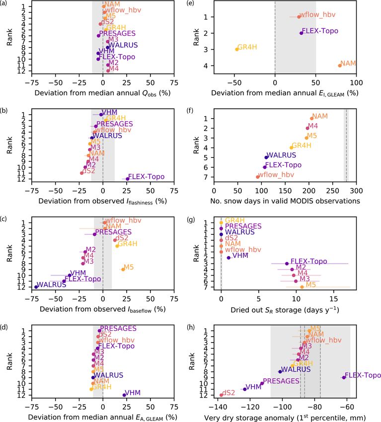
L. J. E. Bouaziz et al.: Behind the scenes of streamflow model performance                                                 1071

   Here, in this model comparison study, we instead use glob-
ally available remote-sensing data to evaluate five different
model state and flux variables of 12 process-based mod-
els with similar overall streamflow performance, which are
calibrated by several research groups following an identi-
cal protocol. The calibration on streamflow was conducted
in our previous study (de Boer-Euser et al., 2017), in which
we compared models using hourly streamflow observations,
leaving the modeled response of internal processes unused.
   In a direct follow-up to the above study, we here hypoth-
esize that process-based models with similar overall stream-
flow performance rely on similar representations of their in-
ternal states and fluxes. We test our hypothesis by simulta-
neously quantifying the differences in the magnitudes and
dynamics of five internal state and flux variables of 12 mod-
els, in a comprehensive and systematic way. Our primary
aim is to test whether models calibrated to streamflow with
similar high-performance levels in reproducing streamflow
follow similar pathways to do so, i.e., represent the system
in a similar way. A secondary objective is to evaluate the
plausibility of model behavior by introducing a set of “soft”
measures based on expert knowledge in combination with
remote-sensing data of evaporation, snow cover, soil mois-
ture and total water storage anomalies.                         Figure 1. (a) Location of the study catchments in Belgium, north-
                                                                western Europe. (b) Digital elevation model and catchments of
                                                                the Ourthe upstream of Tabreux (ID1), Ourthe Orientale upstream
                                                                of Mabompré (ID2) and Semois upstream of Membre-Pont (ID3).
2   Study area
                                                                Pixel size of GRACE, GLEAM, MODIS and SCATSAR-SWI1km.
                                                                Colored dots are the streamflow gauging locations, and black dots
We test our hypothesis using data from three catchments in
                                                                are the precipitation stations.
the Belgian Ardennes; all of them are part of the Meuse
River basin in northwestern Europe: the Ourthe upstream
of Tabreux (ID1), the nested Ourthe Orientale upstream of       2000; de Boer-Euser et al., 2017). Mean annual precipita-
Mabompré (ID2) and the Semois upstream of Membre-Pont           tion, potential evaporation and streamflow are 979, 730 and
(ID3), as shown in Fig. 1. The Ardennes Massif and Plateau      433 mm yr−1 , respectively, for the period 2001–2017.
are underlain by relatively impermeable metamorphic Cam-           Nested within the Ourthe catchment (ID1), the Ourthe Ori-
brian rock and Early Devonian sandstone. The pronounced         entale upstream of Mabompré (ID2) is characterized by a
streamflow seasonality of these catchments is driven by high    narrow elevation range from 294 to 662 m, with 65 % of the
summer and low winter evaporation (defined here as the sum      catchment falling within a 100 m elevation band, making this
of all evaporation components including transpiration, soil     catchment suitable for analyzing snow processes modeled by
evaporation, interception, sublimation and open water evap-     lumped models. The Ourthe Orientale upstream of Mabom-
oration when applicable), as precipitation is relatively con-   pré has an area of 317 km2 , which corresponds to 20 % of
stant throughout the year. Snow is not a major component of     the Ourthe area upstream of Tabreux and has similar land
the water balance but occurs almost every year with mean an-    cover fractions. Mean annual precipitation, potential evapo-
nual number of days with precipitation as snow estimated be-    ration and streamflow for the period 2001–2017 are also rel-
tween 35 and 40 d yr−1 (Royal Meteorological Institute Bel-     atively similar, at 1052, 720 and 462 mm yr−1 , respectively.
gium, 2015). Even if mean annual snow storage is relatively        Forest is the main land cover in the Semois upstream of
small, snow can be important for specific events, for exam-     Membre-Pont (ID3), at 56 %, followed by agriculture (18 %
ple, in 2011, when rain on snow caused widespread flooding      pasture and 21 % crop) and 5 % urban cover. The Semois
in these catchments.                                            upstream of Membre-Pont is 24 % smaller than the Ourthe
   The rain-fed Ourthe River at Tabreux (ID1) is fast-          upstream of Tabreux, at 1226 km2 , and elevation ranges be-
responding due to shallow soils and steep slopes in the         tween 176 and 569 m. Mean annual precipitation, potential
catchment. Agriculture is the main land cover (27 % crops       evaporation and streamflow are, respectively, 38 %, 4 % and
and 21 % pasture), followed by 46 % forestry and 6 % ur-        46 % higher in the Semois at Membre-Pont, at 1352, 759 and
ban cover in an area of 1607 km2 and an elevation rang-         634 mm yr−1 .
ing between 107 and 663 m (European Environment Agency,

https://doi.org/10.5194/hess-25-1069-2021                                    Hydrol. Earth Syst. Sci., 25, 1069–1095, 2021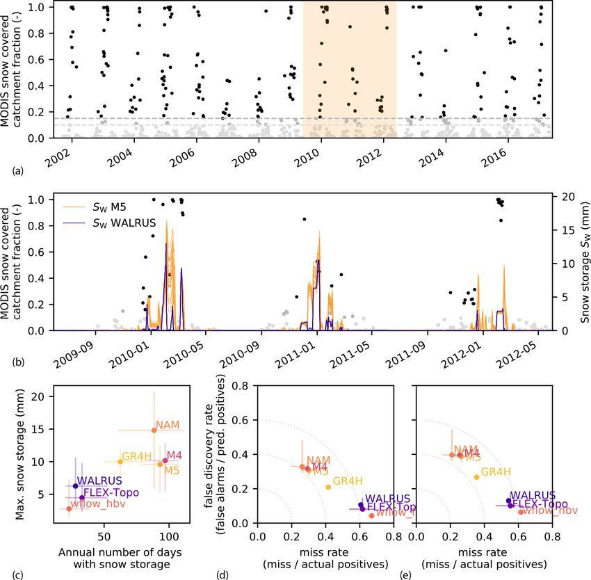
1072                                            L. J. E. Bouaziz et al.: Behind the scenes of streamflow model performance

3     Data                                                        3.2.2   MODIS snow cover

3.1     Hydrological and meteorological data                      The Moderate Resolution Imaging Spectroradiometer
                                                                  (MODIS) AQUA (MYD10A1, version 6) and TERRA
Hourly precipitation gauge data are provided by the Ser-          (MOD10A1, version 6) satellites provide daily maps of
vice Public de Wallonie (Service Public de Wallonie, 2018)        the areal fraction of snow cover per 500 m × 500 m cell
and are spatially interpolated using Thiessen polygons. Daily     (Fig. 1b) based on the Normalized Difference Snow Index
minimum and maximum temperatures are retrieved from               (Hall and Riggs, 2016a, b). For each day, AQUA and
the 0.25◦ resolution gridded E-OBS dataset (Haylock et al.,       TERRA observations are merged into a single observation
2008) and disaggregated to hourly values by linear interpo-       by taking the mean fraction of snow cover per day. The
lation using the timing of daily minimum and maximum ra-          percentage of cells with a fractional snow cover larger than
diation at Maastricht (Royal Netherlands Meteorological In-       zero and fraction of cells without missing data (i.e., due
stitute, 2018). Daily potential evaporation is calculated from    to cloud cover) for the catchment of the Ourthe Orientale
daily minimum and maximum temperatures using the Har-             upstream of Mabompré is calculated for each day. For this
greaves formula (Hargreaves and Samani, 1985) and is dis-         study, we disregard observations during the summer months
aggregated to hourly values using a sine function during the      (JJA, when temperatures did not drop below 4 ◦ C) and
day and no evaporation at night. We use the same forcing for      only use daily observations in which at least 40 % of the
2000–2010 as in the previous comparison study (de Boer-           catchment area has snow cover retrievals not affected by
Euser et al., 2017) and follow the same approach to extend        clouds, implying that we have 1463 valid daily observations
the meteorological dataset for the period 2011–2017. Uncer-       of mean fractional snow cover. This corresponds to 32 % of
tainty in meteorological data is not explicitly considered, but   all observations of the Ourthe Orientale catchment upstream
our primary aim is to compare the models forced with iden-        of Mabompré between 2001 and 2017.
tical data. Observed hourly streamflow data for the Ourthe
at Tabreux, Ourthe Orientale at Mabompré and Semois at            3.2.3   SCATSAR-SWI1km Soil Water Index
Membre-Pont are provided by the Service Public de Wallonie
for the period 2000–2017.                                         SCATSAR-SWI1km is a daily product of soil water content
                                                                  relative to saturation at a 1 km × 1 km resolution (Fig. 1b)
3.2     Remote-sensing data                                       obtained by fusing spatio-temporally complementary radar
                                                                  sensors (Bauer-Marschallinger et al., 2018). Estimates of the
3.2.1    GLEAM evaporation                                        moisture content relative to saturation at various depths in the
                                                                  soil, referred to as the Soil Water Index (SWI), are obtained
The Global Land Evaporation Amsterdam Model (GLEAM,               through temporal filtering of the 25 km METOP ASCAT
Miralles et al., 2011; Martens et al., 2017) provides daily       near-surface soil moisture (Wagner et al., 2013) and 1 km
estimates of land evaporation by maximizing the informa-          Sentinel-1 near-surface soil moisture (Bauer-Marschallinger
tion recovery on evaporation contained in climate and en-         et al., 2018). The Soil Water Index features as a single param-
vironmental satellite observations. The Priestley and Tay-        eter the characteristic time length T (Wagner et al., 1999; Al-
lor (1972) equation is used to calculate potential evapora-       bergel et al., 2008). The T value is required to convert near-
tion for bare soil, short canopy and tall canopy land frac-       surface soil moisture observations to estimates of root-zone
tions. Actual evaporation is the sum of interception and po-      soil moisture. The T value increases with increasing root-
tential evaporation reduced by a stress factor. This evapora-     zone storage capacities (Bouaziz et al., 2020), resulting in
tive stress factor is based on microwave observations of veg-     more smoothing and delaying of the near-surface soil mois-
etation optical depth and estimates of root-zone soil moisture    ture signal. The Copernicus Global Land Service (2019) pro-
in a multi-layer water-balance model. Interception evapora-       vides the Soil Water Index for T values of 2, 5, 10, 15, 20, 40,
tion is estimated separately using a Gash analytical model        60 and 100 d. Since Sentinel-1 was launched in 2014, the Soil
and only depends on precipitation and vegetation charac-          Water Index is available for the period 2015–2017. We cal-
teristics. GLEAM v3.3a relies on reanalysis net radiation         culate the mean soil moisture over all SCATSAR-SWI1km
and air temperature from the European Centre for Medium-          pixels within the Ourthe upstream of Tabreux for the avail-
Range Weather Forecasts (ECMWF) ERA5 data, satellite              able period.
and gauge-based precipitation, satellite-based vegetation op-
tical depth, soil moisture and snow water equivalent. The data    3.2.4   GRACE total water storage anomalies
are available at 0.25◦ resolution (Fig. 1b) and account for
subgrid heterogeneity by considering three land cover types.      The Gravity Recovery and Climate Experiment (GRACE,
We spatially average GLEAM interception and total actual          Swenson and Wahr, 2006; Swenson, 2012) twin satellites,
evaporation estimates over the Ourthe catchment upstream          launched in March 2002, measure the Earth’s gravity field
of Tabreux for the period 2001–2017.                              changes by calculating the changes in the distance between

Hydrol. Earth Syst. Sci., 25, 1069–1095, 2021                                      https://doi.org/10.5194/hess-25-1069-2021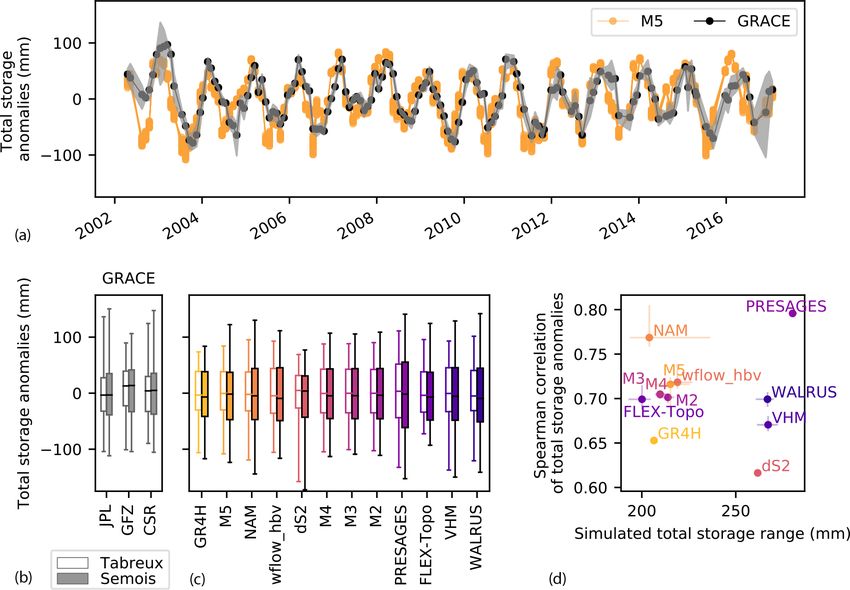
L. J. E. Bouaziz et al.: Behind the scenes of streamflow model performance                                                   1073

the two satellites as they move one behind the other in the        datasets, as shown by Miralles et al. (2016). GLEAM inter-
same orbital plane. Monthly total water storage anomalies          ception currently only considers tall vegetation and under-
(in millimeters) relative to the 2004–2009 time-mean base-         estimates in situ data (Zhong et al., 2020) and is ∼ 50 %
line are provided at a spatial sampling of 1◦ (approximately       lower than estimates from other datasets (Miralles et al.,
78 km × 110 km at the latitude of the study region, Fig. 1b)       2016). These uncertainties underline that GLEAM (and other
by three centers: U. Texas/Center for Space Research (CSR),        remote-sensing data) cannot be considered a reliable repre-
GeoForschungsZentrum Potsdam (GFZ) and Jet Propulsion              sentation of real-world quantities. However, the comparison
Laboratory (JPL). These centers apply different processing         of daily dynamics and absolute values of this independent
strategies which lead to variations in the gravity fields. These   data source with modeled results is still valuable for detect-
gravity fields require smoothing of the noise induced by at-       ing potential outliers and understanding their behavior. In ad-
tenuated short wavelength. The spatial smoothing decreases         dition, the different methods used to estimate potential evap-
the already coarse GRACE resolution even further through           oration of GLEAM and our model forcing should not impede
signal “leakage” of one location to surrounding areas (Bonin       us from testing the consistency between the resulting actual
and Chambers, 2013), which increases the uncertainty espe-         evaporation (Oudin et al., 2005).
cially at the relatively small scale of our study catchments.         The most frequent errors within the MODIS snow cover
We apply the scaling coefficients provided by NASA to re-          products are due to cloud–snow discrimination problems.
store some of the signal loss due to processing of GRACE           Daily MODIS snow maps have an accuracy of approximately
observations (Landerer and Swenson, 2012). The data of the         93 % at the pixel scale, with lower accuracy in forested areas
three processing centers are each spatially averaged over the      and complex terrain and when snow is thin and ephemeral
catchments of the Ourthe upstream of Tabreux and the Se-           and higher accuracy in agricultural areas (Hall and Riggs,
mois upstream of Membre-Pont for the period April 2002 to          2007). However, here, MODIS data are used to estimate the
February 2017.                                                     number of days with snow at the catchment scale. We expect
                                                                   lower classification errors at the catchment scale as it would
3.3   Data uncertainty                                             require many pixels to be misclassified at the same time. For
                                                                   each day and each pixel of valid MODIS observations, we
The hydrological evaluation data are all subject to uncertain-     sample from a binomial distribution with a probability of
ties (Beven, 2019). Streamflow is not measured directly but        93 % that MODIS is correct when the pixel is classified as
depends on water level measurements and a rating curve.            snow and assume a higher probability of 99 % that MODIS
Westerberg et al. (2016) quantify median streamflow uncer-         is correct when the pixel is classified as no-snow to prevent
tainties of ±12 %, ±24 % and ±34 % for average, high and           overestimation of snow for days without snow (Ault et al.,
low streamflow conditions, respectively, using a Monte Carlo       2006; Parajka and Blöschl, 2006). We repeat the experiment
sampling approach of multiple feasible rating curves for 43        1000 times in a Monte Carlo procedure. This results in less
UK catchments. We sample from these uncertainty ranges to          than ±2 % uncertainty in the number of days when MODIS
transform the streamflow observations (100 realizations). We       observes snow at the catchment scale.
then quantify signature uncertainty originating from stream-          The soil water content relative to saturation of SCATSAR-
flow data uncertainty using the 100 sampled time series for a      SWI1km is estimated from observed radar backscatter
selection of streamflow signatures (Sect. 4.2). The 5th–95th       through a change detection approach, which interprets
uncertainty bounds of median annual streamflow, baseflow           changes in backscatter as changes in soil moisture, while
and flashiness indices result in ±11 %, ±9 % and ±12 %, re-        other surface properties are assumed static (Wagner et al.,
spectively. These magnitudes are similar to those reported by      1999). The degree of saturation of the near surface is given
Westerberg et al. (2016).                                          in relative units from 0 % (dry reference) to 100 % (wet refer-
   GLEAM evaporation estimates are inferred from models            ence) and is converted to deeper layers through an exponen-
and forcing data which are all affected by uncertainty. Yet        tial filter called the Soil Water Index. The smoothing and de-
uncertainty estimates of GLEAM evaporation are not avail-          laying effect of the Soil Water Index narrows the range of the
able. However, GLEAM evaporation was evaluated against             near-surface degree of saturation. Therefore, data matching
FLUXNET data by Miralles et al. (2011). For the nearby sta-        techniques are often used to rescale satellite data to match the
tion of Lonzee in Belgium, they report similar annual rates        variability of modeled or observed data (Brocca et al., 2010),
and a high correlation coefficient of 0.91 between the daily       which suggests the difficulty in meaningfully comparing the
time series. GLEAM mean annual evaporation was compared            range of modeled and remote-sensing estimates of root-zone
to the ensemble mean of five evaporation datasets in Miralles      soil moisture content relative to saturation. However, the
et al. (2016) and shows higher than average values in Europe       dynamics of SCATSAR-SWI1km data have been evaluated
(of approximately 60 mm yr−1 or 10 % of mean annual rates          against in situ stations of the International Soil Moisture Net-
for our study area). The partitioning of evaporation into dif-     work, despite commensurability issues of comparing in situ
ferent components (transpiration, interception and soil evap-      point measurements and areal satellite data. Spearman rank
oration) differs substantially between different evaporation       correlation coefficients of 0.56 are reported for T values up to

https://doi.org/10.5194/hess-25-1069-2021                                       Hydrol. Earth Syst. Sci., 25, 1069–1095, 2021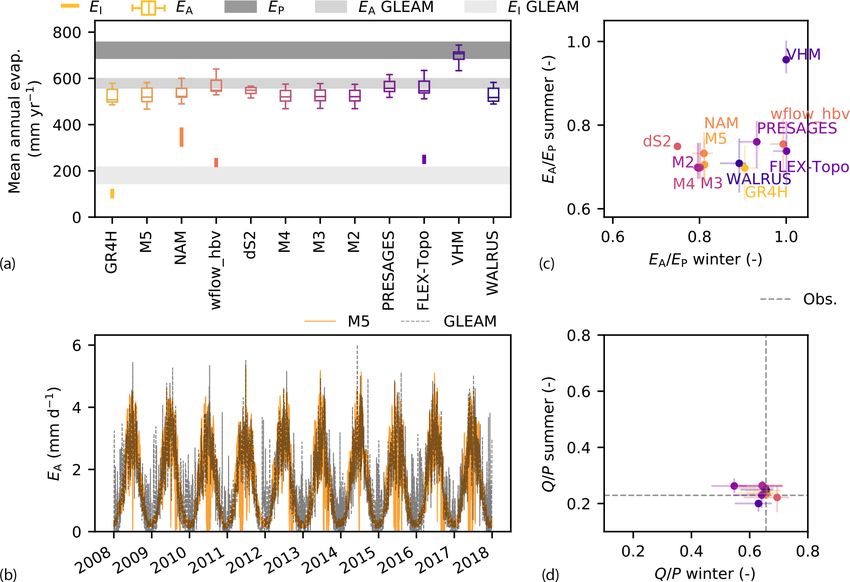
1074                                           L. J. E. Bouaziz et al.: Behind the scenes of streamflow model performance

15 d and 0.43 for a T value of 100 d (Bauer-Marschallinger,      ward. The models were previously calibrated using stream-
2020).                                                           flow of the Ourthe at Tabreux (ID1) for the period 2004 to
   GRACE estimates of total water storage anomalies suf-         2007, using 2003 as a warm-up year (de Boer-Euser et al.,
fer from signal degradation due to measurement errors and        2017). The Nash–Sutcliffe efficiencies of the streamflow and
noise. Filtering approaches are applied to reduce these errors   the logarithms of the streamflow were simultaneously used as
but induce leakage of signals from surrounding areas. The        objective functions to select an ensemble of 20 feasible pa-
uncertainty decreases as the size of the region under con-       rameter sets to account for parameter uncertainty and ensure
sideration increases. However, time series of a single pixel     a balance between the models’ ability to reproduce both high
may still be used to compare dynamics and amplitudes of to-      and low flows. The temporal and spatial transferability of the
tal water storage anomalies despite possible large uncertainty   models was tested by evaluating the models in a pre- and
(Landerer and Swenson, 2012). We estimate an uncertainty         post-calibration period and by applying the calibrated model
in total water storage anomalies of ∼ 18 mm in the pixels        parameter sets to nested and neighboring catchments, includ-
of our catchments by combining measurement and leakage           ing catchment ID2 and ID3 (Klemeš, 1986). Results thereof
errors in quadrature, which are both provided for each grid      are presented in de Boer-Euser et al. (2017).
location (Landerer and Swenson, 2012).                              In the current study, we run the calibrated models for
                                                                 an additional period from 2011 to 2017 for the Ourthe at
                                                                 Tabreux (ID1), the Ourthe Orientale at Mabompré (ID2) and
4     Methods                                                    the Semois at Membre-Pont (ID3). Note that the calibration
                                                                 (2004–2007) and post-calibration (2008–2017) periods have
4.1    Models and protocol                                       relatively similar hydro-climatic characteristics in terms of
                                                                 streamflow and overall water balance (Figs. S1 and S2 of the
Eight research groups (Wageningen University, Université         Supplement). The modeling groups have provided simulation
de Lorraine, Leuven University, Delft University of Tech-        results for each catchment in terms of streamflow, groundwa-
nology, Deltares, Irstea (now INRAE), Eawag and Flan-            ter losses/gains, interception evaporation, root-zone evapora-
ders Hydraulics Research) participated in the comparison         tion (transpiration and soil evaporation), total actual evapo-
experiment and applied one or several hydrological models        ration, snow storage, root-zone storage and total storage as a
(Fig. 2). The models include WALRUS (Wageningen Low-             sum of all model storage volumes (Table 2) at an hourly time
land Runoff Simulator, Brauer et al., 2014a, b), PRESAGES        step for the total period 2001–2017. We compare these mod-
(PREvision et Simulation pour l’Annonce et la Gestion des        eled states and fluxes and evaluate them against their remote-
Etiages Sévères, Lang et al., 2006), VHM (Veralgemeend           sensing equivalents as further explained in Sects. 4.2 and
conceptueel Hydrologisch Model, Willems, 2014), FLEX-            4.3. Our results are mainly shown for the Ourthe at Tabreux
Topo, which was still under development when it was cali-        (ID1), as this catchment was used for calibration of the mod-
brated for our previous study (Savenije, 2010; de Boer-Euser     els. However, the snow analysis is performed for catchment
et al., 2017; de Boer-Euser, 2017), a distributed version of     ID2 due to the narrower elevation range. Catchments ID1 and
the HBV model (Hydrologiska Byråns Vattenbalansavdel-            ID3 are used to analyze the spatial variability of total storage
ning, Lindström et al., 1997), the SUPERFLEX M2 to M5            anomalies.
models (Fenicia et al., 2011, 2014), dS2 (distributed simple
dynamical systems, Buitink et al., 2020), GR4H (Génie Ru-        4.2   Model evaluation: water balance
ral à 4 paramètres Horaire, Mathevet, 2005; Coron et al.,
2017, 2019) combined with the CemaNeige snow mod-                All the models are evaluated in terms of the long-term water
ule (Valéry et al., 2014) and NAM (NedborAfstrommings            balance, which indicates the partitioning between drainage
Model, Nielsen and Hansen, 1973). The main differences and       and evaporative fluxes and allows us to assess long-term con-
similarities between the models in terms of snow processes,      servation of water and energy. We compare mean annual
root-zone storage, total storage and evaporation processes are   streamflow with observations and mean annual actual evap-
summarized in Tables 1–3.                                        oration and interception evaporation with GLEAM estimates
   In our previous study (de Boer-Euser et al., 2017), we de-    for the Ourthe at Tabreux during the evaluation period 2008–
fined a modeling protocol to limit the degrees of freedom in     2017. A detailed description of streamflow performance for
the modeling decisions of the individual participants (Ceola     specific events (low and high flows, snowmelt events, tran-
et al., 2015), allowing us to meaningfully compare the model     sition from dry to wet periods) has been detailed in the
results. The protocol involved forcing the models with the       previous paper (de Boer-Euser et al., 2017). In the current
same input data and calibrating them for the same time pe-       study, differences in streamflow dynamics are briefly sum-
riod, using the same objective functions. However, partici-      marized by assessing observed and modeled baseflow indices
pants were free to choose a parameter search method, as we       (Ibaseflow , van Dijk, 2010) and flashiness indices (Iflashiness ,
considered it to be part of the modelers’ experience with the    Fenicia et al., 2016), as these are representative of the parti-
model, even if this would make comparison less straightfor-      tioning of drainage into fast and slow responses. Seasonal dy-

Hydrol. Earth Syst. Sci., 25, 1069–1095, 2021                                     https://doi.org/10.5194/hess-25-1069-2021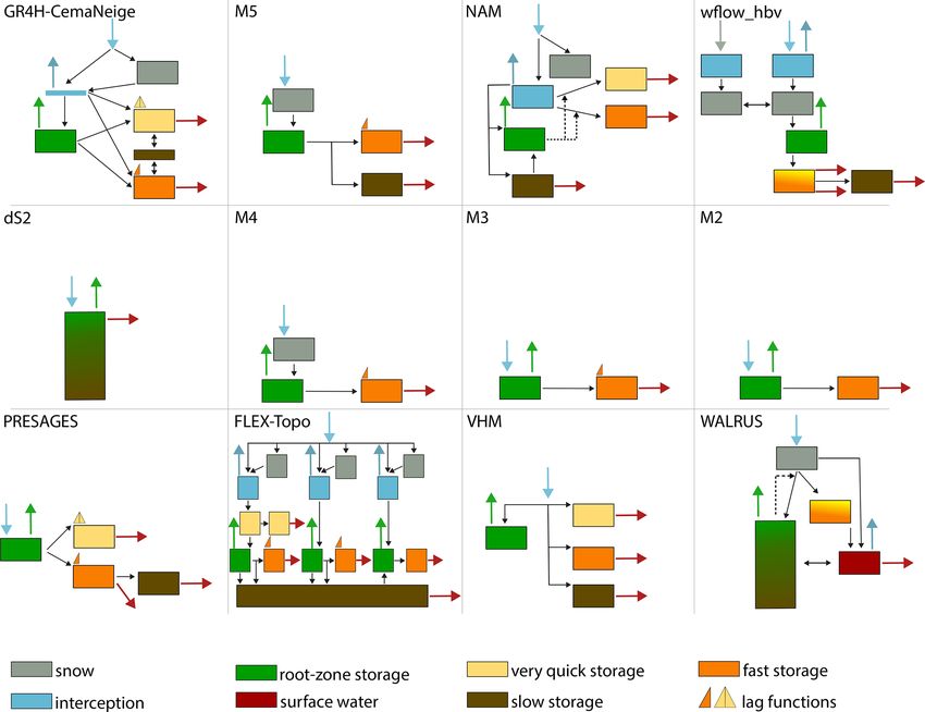
L. J. E. Bouaziz et al.: Behind the scenes of streamflow model performance                                                              1075

Table 1. Description of symbols used for fluxes, storages and parameters in Tables 2 and 3.

     Symbol        Unit        Description
     Fluxes
     EP            mm h−1      Potential evaporation
     EI            mm h−1      Interception evaporation
     ER            mm h−1      Transpiration and soil evaporation
     EW            mm h−1      Sublimation
     EA            mm h−1      Total actual evaporation (sum of soil evaporation, transpiration, (separate) interception and, if applica-
                               ble, sublimation)
     P             mm h−1      Precipitation
     PR            mm h−1      Precipitation entering the root-zone storage (after snow and/or interception if present or fraction/total
                               precipitation)
     Q             mm h−1      Streamflow
     QR            mm h−1      Flux from root zone to fast and/or slow runoff storage
     QP            mm h−1      Percolation flux from root-zone storage to slow runoff storage
     QC            mm h−1      Capillary flux from slow runoff storage to root-zone storage
     QG            mm h−1      Seepage (up/down)/extraction
     Storages
     ST            mm          Total storage
     SW            mm          Snow storage
     SI            mm          Interception storage
     SR            mm          Root-zone storage
     SR            –           Relative root-zone storage (SR /SR,max )
     SD            mm          Storage deficit
     SVQ           mm          Very quick runoff storage
     SF            mm          Fast runoff storage
     SS            mm          Slow runoff storage
     SSW           mm          Surface water storage
     Parameters
     CE            –           Correction factor for EP
     Imax          mm          Maximum interception capacity
     SR,max        mm          Maximum root-zone storage capacity
     Sthresh       mm          Threshold of root-zone storage above which ER = EP
     LP            –           Threshold of relative root-zone storage above which ER = EP
     Ccst          –           Constant water stress coefficient to estimate ER
     a, b, S0      –           Parameters describing the shape of the streamflow sensitivity
     aS            –           Fraction of land surface covered by surface water
     aG            –           Fraction of land surface not covered by surface water

https://doi.org/10.5194/hess-25-1069-2021                                               Hydrol. Earth Syst. Sci., 25, 1069–1095, 2021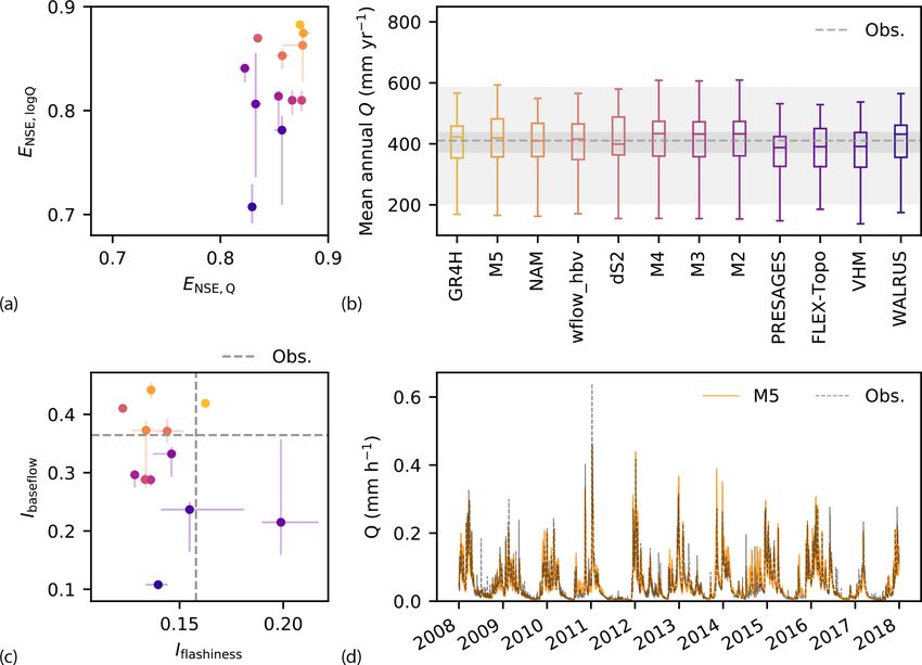
L. J. E. Bouaziz et al.: Behind the scenes of streamflow model performance
https://doi.org/10.5194/hess-25-1069-2021
Table 2. Number of calibrated model parameters, spatial distribution, and model performance calculated for the period 2008–2017 with the Euclidean distance where a value of 0 would
indicate a perfect model. Main characteristics describing snow storage, root-zone storage and total storage per model. Notations are defined in Table 1.
GR4H M5 NAM wflow_hbv dS2 M4 M3 M2 PRESAGES FLEX-Topo VHM WALRUS
Number of calibrated parameters 4 9 12 9 4 7 6 5 6 20 12 3
Lumped (L)/semi-distributed (S)/distributed (D)
q L L L D L L L L L S L L
Euclidean distance (1 − ENS,Q )2 + (1 − ENS,logQ )2 0.17 0.18 0.18 0.20 0.21 0.23 0.23 0.24 0.24 0.26 0.26 0.34
Snow storage SW (compared to MODIS snow cover)
Snow module X X X X – X – – – X – X
Degree-hour method X X X X – X – – – X – X
Elevation zones X – – X – – – – – X – –
Temperature interval for rainfall and snow X – – X – – – – – X – X
Melt factor constant in time – X – X – X – – – X – X
Melt factor ∼ snow storage X – X – – – – – – – – –
Refreezing of liquid water – – X X – – – – – – – –
Sublimation – – – – – – – – – X – –
Calibration snow parameters – X X – – X – – – X – –
Root-zone storage SR (compared to SCATSAR-SWI1km Soil Water Index)
Separate root-zone module with capacity SR,max X X X X – X X X X X X –
dSR
dt = PR − ER – – – – – – – – – – X –
dSR
dt = PR − ER + QC – – X – – – – – – – – –
dSR
= PR − ER − QR X X – X – X X X X – – –
Hydrol. Earth Syst. Sci., 25, 1069–1095, 2021
dt
dSR
dt = PR − ER − QR − −QP + QC – – – – – – – – – X – –
Total storage ST (anomalies are compared to GRACE total storage anomalies)
ST = −SD · aG + SF · aG + SSW · aS – – – – – – – – – – – X
ST (Q) = a1 1−b
1 · Q1−b + S
0 – – – – X – – – – – – –
ST = SR + SF – – – – – – X X – – – –
ST = SW + SR + SF – – – – – X – – – – – –
ST = SW + SR + SF + SS – X – – – – – – – – – –
ST = SR + SVQ + SF + SS – – – – – – – – X – X –
ST = SW + SR + SVQ + SF + SS X – – – – – – – – – – –
ST = SI + SW + SR + SF + SS – – – X – – – – – – – –
ST = SI + SW + SR + SVQ + SF + SS – – X – – – – – – X – –
1076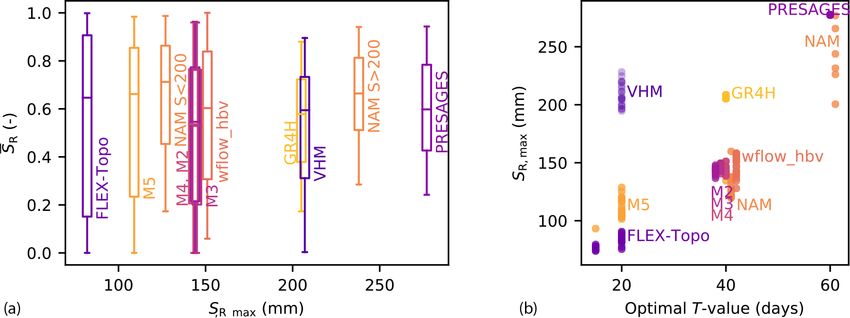
L. J. E. Bouaziz et al.: Behind the scenes of streamflow model performance                                                              1077

Figure 2. Simplified schematic overview of 12 model structures (adapted from de Boer-Euser et al., 2017) with the aim of highlighting
similarities and differences between the models. Solid arrows indicate fluxes between stores, while dashed arrows indicate the influence of a
state on a flux. Colored arrows indicate incoming or outgoing fluxes, whereas black arrows indicate internal fluxes. The narrow blue rectangle
in GR4H indicates the presence of an interception module without interception storage capacity (Table 3). Storages with a color gradient
indicate the combination of several components in one reservoir. FLEX-Topo consists of three hydrological response units connected through
a shared slow reservoir, and wflow_hbv is a distributed model.

namics of actual evaporation over potential evaporation and              sified as days with and without snow using thresholds of
runoff coefficients during winter (October–March) and sum-               both 10 % and 15 % of snow-covered cells in the catchment
mer (April–September) are compared between the models.                   to be counted as a day with snow, in a sensitivity analysis.
                                                                         For each model, snow days are distinguished from non-snow
4.3     Model evaluation: internal states                                days whenever the water stored as snow is above 0.05 mm to
                                                                         account for numerical rounding. For each model (and each
We compare modeled snow storage, root-zone soil mois-                    retained parameter set), we then compare whether modeled
ture and total storage between the models and with remote-               snow coincides with “truly” observed snow by MODIS, for
sensing estimates of MODIS snow cover, SCATSAR-                          each day with a valid MODIS observation. We create a con-
SWI1km Soil Water Index and GRACE total storage anoma-                   fusion matrix with counts of true positives when observations
lies, respectively, as shown in Tables 2–3.                              and model results agree on the presence of snow (hits), false
                                                                         positives when the model indicates the presence of snow but
4.3.1    Snow days
                                                                         this is not observed by MODIS (false alarms), false nega-
As most models used in this study are lumped, it is not possi-           tives when the model misses the presence of snow observed
ble to spatially evaluate modeled snow cover versus MODIS                by MODIS (miss) and true negatives when observations and
snow cover. However, we can classify each day in a binary                model results agree on the absence of snow (correct rejec-
way according to the occurrence of snow, based on a thresh-              tions). This allows us to identify the trade-off between, on the
old for the percentage of cells in the catchment where snow              one hand, the miss rate between model and remote-sensing
cover is detected. MODIS snow cover observations are clas-               observation, as the ratio of misses over actual positives (num-

https://doi.org/10.5194/hess-25-1069-2021                                               Hydrol. Earth Syst. Sci., 25, 1069–1095, 2021
L. J. E. Bouaziz et al.: Behind the scenes of streamflow model performance
https://doi.org/10.5194/hess-25-1069-2021
Table 3. Main characteristics describing evaporation processes per model (where X1 indicates LP = 1 and X2 indicates EI = 0). Notations are defined in Table 1.
GR4H M5 NAM wflow_hbv dS2 M4 M3 M2 PRESAGES FLEX-Topo VHM WALRUS
Correction factor for potential evaporation – X – – – X X X – – – –
Interception evaporation EI X – X X – – – – – X – –
Maximum interception storage Imax – – X X – – – – – X – –
Imax ∼ 1.1 − 3.4 mm – – – – – – – – – X – –
Imax ∼ 1.4 − 2.9 mm – – – X – – – – – – – –
Imax ∼ 5.3 − −6.9 mm
( – – X – – – – – – – – –
E , if SI > 0.
P
EI = – – X X – – – – – X – –
(0, otherwise.
EP , if P > EP .
EI = X – – – – – – – – – – –
P , otherwise.
Transpiration and soil evaporation ER X X X X X X X X X X X X
ER = EP · Ccst – – – – X – – – – – – –
S R ·(2−S R )
ER = EP · X – – – – – – – X – – –
1+EP /SR,max ·(2−S R )
ER = EP · CE · S R ·(1+m1 ) , with m1 = 10−2 – X – – – X X X – – – –
S R +m1
Hydrol. Earth Syst. Sci., 25, 1069–1095, 2021
(
SR
(EP − EI ) · L , if S R < LP .
ER = P – – X1 X – – – – – X X2 –
EP − EI , otherwise.
ER = EP · f(Sd ) – – – – – – – – – – – X
Total actual evaporation EA X X X X X X X X X X X X
EA = ER – X – – X X X X X – X X
EA = ER + EI X – X X – – – – – – – –
EA = ER + EI + EW – – – – – – – – – X – –
1078L. J. E. Bouaziz et al.: Behind the scenes of streamflow model performance 1079
ber of days when snow is observed by MODIS) and, on the ments coincide with two neighboring GRACE cells, allowing
other hand, the false discovery rate as the ratio of false alarms us to test how well the models reproduce the observed spatial
over predicted positives (number of days when snow is mod- variability. We further relate the modeled range of total stor-
eled). We also compare annual maximum snow storage and age (maximum minus minimum total storage over the time
number of days with snow between the seven models with a series) to Spearman rank correlation coefficients between
snow module (GR4H, M5, NAM, wflow_hbv, M4, FLEX- modeled and GRACE estimates of total storage anomalies.
Topo, WALRUS). The snow analysis is performed in the
catchment of the Ourthe Orientale upstream of Mabompré 4.4 Interactions between storage and fluxes during dry
as it features the narrowest elevation range among the study periods
catchments (i.e., 294–662 m a.s.l. versus 108–662 m for the
Ourthe upstream of Tabreux) and thus plausibly permits a The impact of a relatively large (> 200 mm) versus relatively
lumped representation of the snow component. small (< 150 mm) root-zone storage capacity on actual evap-
oration, streamflow and total storage is assessed during a
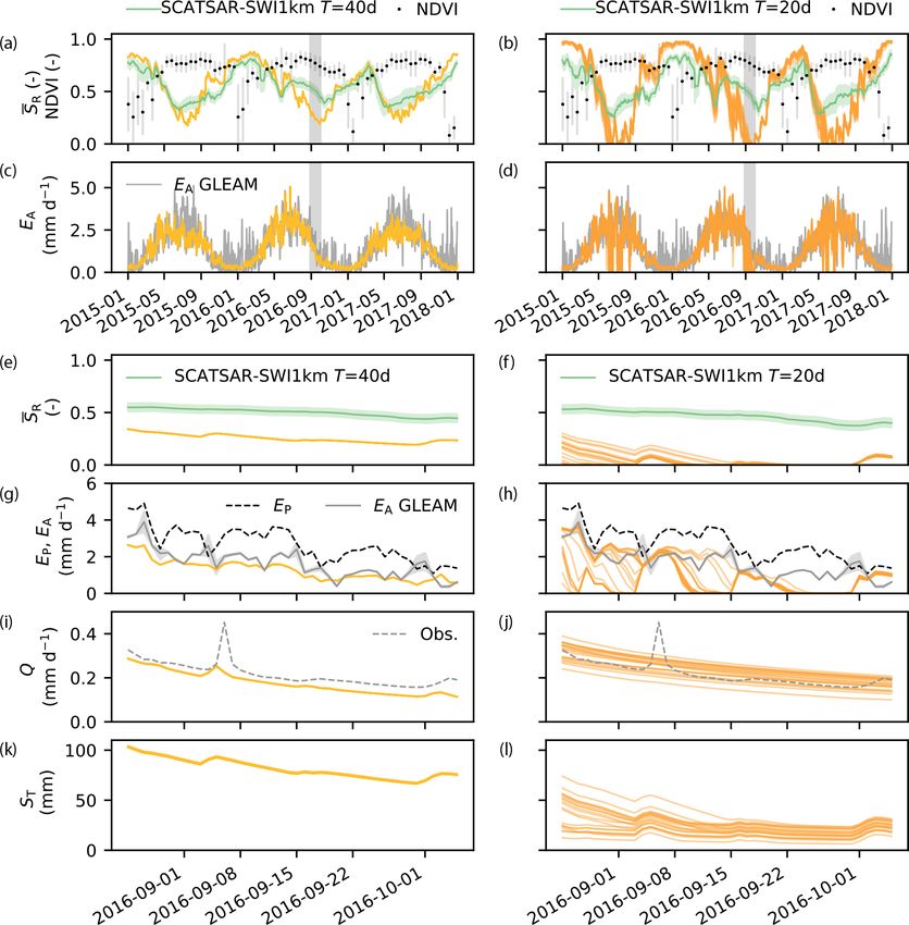
4.3.2 Root-zone soil moisture dry period in September 2016 by selecting two representa-
tive models with high streamflow model performance (GR4H
We compare the range of the relative root-zone soil mois- and M5). The plausibility of the hydrological response of
ture S R (S R = SR /SR,max , Table 1) between the models for these two model representations is evaluated against remote-
the period in which SCATSAR-SWI1km is available (2015– sensing estimates of root-zone soil moisture and actual evap-
2017). Time series of catchment-scale root-zone soil mois- oration.
ture are available for all the models except WALRUS and
dS2 as these models have a combined soil reservoir (Fig. 2). 4.5 Plausibility of process representations
The dS2 model only relies on the sensitivity of streamflow
The models are subsequently ranked and evaluated in terms
to changes in total storage. In WALRUS, the state of the
of their consistency with observed streamflow, remote-
soil reservoir (which includes the root zone) is expressed
sensing data and expert knowledge with due consideration of
as a storage deficit and is therefore not bound by an upper
the uncertainty in the evaluation data, as detailed in Sect. 3.3.
limit (Table 2). Root-zone storage capacities (SR,max , mm)
We summarize our main findings by evaluating the models in
are available as a calibration parameter for all the other mod-
terms of their deviations around median annual streamflow,
els. We relate the range in relative root-zone soil moisture to
flashiness and baseflow indices, median annual actual evap-
the maximum root-zone storage capacity SR,max , because we
oration and interception compared to GLEAM estimates, the
expect models with small root-zone storage capacities SR,max
number of days with snow over valid MODIS observations,
to entirely utilize the available storage through complete dry-
the number of days per year with empty root-zone stor-
ing and saturation.
age and the very dry total storage anomalies compared to
We then compare the similarity of the dynamics of mod-
GRACE estimates.
eled time series of the relative root-zone soil moisture with
the remotely sensed SCATSAR-SWI1km Soil Water Index
for several values of the characteristic time length parame- 5 Results and discussion
ter (T in days). The T value has previously been positively
correlated with root-zone storage capacity, assuming a high 5.1 Water balance
temporal variability of root-zone soil moisture and therefore
a low T value for small root-zone storage capacities SR,max 5.1.1 Streamflow
(Bouaziz et al., 2020). For each model and feasible realiza-
tion, we identify the T value that yields the highest Spear- All the models show high Nash–Sutcliffe efficiencies of the
man rank correlation between modeled root-zone soil mois- streamflow and the logarithm of the streamflow (ENS,Q and
ture and Soil Water Index. We then relate the optimal T value ENS,logQ ) with median values of above 0.7 for the post-
to the root-zone storage capacity SR,max . This analysis en- calibration evaluation period 2008–2017 (Fig. 3a and Table 2
ables us to identify potential differences in the representation for the calculation of the Euclidean distances). The interan-
and the dynamics of root-zone storage between the models. nual variability of streamflow agrees strongly with observa-
tions for each model in the period 2008–2017 (Fig. 3b). The
4.3.3 Total storage anomalies difference between modeled and observed median stream-
flow varies between −5.6 % and 5.6 %, and the difference
For each model, we calculate time series of total storage (Ta- in total range varies between −9.6 % and 20 %. This is in
ble 2) and mean monthly total storage anomalies relative line with our results in the previous paper, in which we
to the 2004–2009 time-mean baseline for comparison with also showed that all the models perform well in terms of
GRACE estimates for the Ourthe upstream of Tabreux (ID1) commonly used metrics (de Boer-Euser et al., 2017). How-
and the Semois upstream of Membre-Pont (ID3). Both catch- ever, there are differences in the partitioning of fast and
https://doi.org/10.5194/hess-25-1069-2021 Hydrol. Earth Syst. Sci., 25, 1069–1095, 20211080 L. J. E. Bouaziz et al.: Behind the scenes of streamflow model performance
slow runoff, as shown by the flashiness and baseflow indices 1980) and 50 % for a forest in Puerto Rico (Schellekens et al.,
(Iflashiness and Ibaseflow ) in Fig. 3c. The largest underestima- 1999), and are difficult to extrapolate to other catchments due
tion of the flashiness index occurs for M2 and dS2 (∼ 20 %), to the heterogeneity and complexity of natural systems.
while FLEX-Topo shows the highest overestimation (26 %). GLEAM estimates of actual evaporation show relatively
FLEX-Topo and WALRUS underestimate the baseflow in- high evaporation rates in winter and are never reduced to zero
dex most (41 % and 70 %, respectively), while GR4H and in summer, as opposed to modeled M5 estimates, as shown
M5 show the highest overestimation (15 % and 21 %, respec- in Fig. 4b. GLEAM actual evaporation minus the separately
tively). There is a strong similarity between modeled and ob- calculated interception is 94 % of potential evaporation, im-
served hydrographs for one of the best performing models plying almost no water-limited conditions, as opposed to
M5, as quantified by its low Euclidean distance (Fig. 3d and our models in which actual evaporation in summer (April–
Table 2). The GR4H model is the only one which includes September) is, due to water stress, reduced to approximately
deep groundwater losses, but they are very limited and rep- 73 % of potential evaporation on average for all the models
resent only 1.6 % of total modeled streamflow of the Ourthe except VHM (Fig. 4c). Larger differences between the mod-
at Tabreux, or approximately 7 mm yr−1 . els occur in the ratio EA /EP during winter (October–March),
when FLEX-Topo, wflow_hbv and VHM show EA /EP ratios
5.1.2 Actual evaporation close to unity and dS2 the lowest values of EA /EP ∼ 0.75 as
shown in Fig. 4c. The dS2 model differs from all the other
Modeled median annual actual evaporation EA (computed models as it relies on a year-round constant water stress co-
as the sum of soil evaporation, transpiration, (separate) inter- efficient (Ccst ), independent of water supply, while the stress
ception evaporation and, if applicable, sublimation, Table 3) coefficient depends on root-zone soil moisture content in all
for hydrological years between October 2008 and Septem- the other models (Table 3).
ber 2017 varies between 507 and 707 mm yr−1 across mod- Most models slightly overestimate summer runoff coeffi-
els, with a median of 522 mm yr−1 , which is approximately cients, with values between 0.22 and 0.26, which are very
10 % lower than the GLEAM estimate of 578 mm yr−1 , as close to the observed value of 0.22, as shown in Fig. 4d. Dur-
shown in Fig. 4a. Annual actual evaporation of the VHM ing winter, runoff coefficients vary between 0.55 and 0.71,
model is very high compared to the other models, with a which is close to the observed value of 0.66. This implies a
median of 707 mm yr−1 , and approximates potential evap- relatively high level of agreement between the models in re-
oration (median of 732 mm yr−1 ). Calibration of the VHM producing the medium- to long-term partitioning of precipi-
model is meant to follow a manual stepwise procedure in- tation into evaporation and drainage and thus in approximat-
cluding the closure of the water balance during the identifi- ing at least long-term conservation of energy (Hrachowitz
cation of soil moisture processes (Willems, 2014). However, and Clark, 2017).
in the automatic calibration prescribed by the current proto-
col, this step was not performed, which explains the unusual 5.2 Internal model states
high actual evaporation in spite of relatively similar annual
streamflow compared to the other models, as there is no clo- 5.2.1 Snow days
sure of the water balance (Fig. 3a).
Interception evaporation is included in four models, with MODIS snow cover is detected over most of the catchment
GR4H showing the lowest annual interception evaporation area for some time each year between November 2001 and
of 100 mm yr−1 (19 % of EA or 10 % of P ), FLEX-Topo November 2017, except for the periods of November 2006
and wflow_hbv having relatively similar amounts of approx- to March 2007 and November 2007 to March 2008, when
imatively 250 mm yr−1 (∼ 45 % of EA or 26 % of P ) and snow is detected in less than half of the catchment cells, as
NAM having the highest annual interception evaporation of shown in Fig. 5a. The number and magnitude of modeled
340 mm yr−1 (65 % of EA or 36 % of P ), as shown in Fig. 4a. snow storage events varies between the models (Fig. 5b). The
Differences are related to the presence and maximum size of modeled number of snow days per hydrological year varies
the interception storage (Imax ), as shown in Table 3. GLEAM from ∼ 28 d for FLEX-Topo, WALRUS and wflow_hbv to
interception estimates of 189 mm yr−1 are almost twice as ∼ 62 d for GR4H and ∼ 90 d for NAM, M4 and M5, as shown
high as GR4H estimates, 25 % lower than FLEX-Topo and in Fig. 5c. The variability in median annual maximum snow
wflow_hbv, and 44 % lower than NAM values, suggesting a storage varies from 3 mm for wflow_hbv and ∼ 5–6 mm for
large uncertainty in the contribution of interception and tran- FLEX-Topo and WALRUS to ∼ 10 mm for GR4H, M4, and
spiration to actual evaporation. For comparison, measure- M5 and 15 mm for NAM. We further evaluate the plausibility
ments of the fraction of interception evaporation over precip- of these modeled snow processes by comparing modeled and
itation in forested areas vary significantly depending on the observed snow cover for days when a valid MODIS observa-
site location, with estimates of 37 % for a Douglas fir stand in tion is available.
the Netherlands (Cisneros Vaca et al., 2018), 27 %, 32 % and The presence of snow modeled by FLEX-Topo,
42 % for three coniferous forests of Great Britain (Gash et al., wflow_hbv and WALRUS coincides for 92 % with the
Hydrol. Earth Syst. Sci., 25, 1069–1095, 2021 https://doi.org/10.5194/hess-25-1069-2021L. J. E. Bouaziz et al.: Behind the scenes of streamflow model performance 1081 Figure 3. Evaluation of modeled streamflow performance for the Ourthe at Tabreux for the period 2008–2017. (a) Nash–Sutcliffe efficiencies of the streamflow ENS,Q and the logarithm of the streamflow ENS,logQ (median, 25th/75th percentiles across parameter sets). (b) Modeled mean annual streamflow for hydrological years between 2008 and 2017 across feasible parameter sets. The models are ranked from the highest to the lowest performance according to the Euclidean distance of streamflow performance (see Table 2). The dashed line and grey shaded areas show median, 25th/75th and minimum–maximum range of observed mean annual streamflow. (c) Baseflow index Ibaseflow as a function of the flashiness index Iflashiness (median, 25th/75th percentiles across parameter sets). Observed values are shown by the grey dashed lines. (d) Observed and modeled hydrographs of model M5 with high streamflow model performance (low Euclidean distance). presence of snow observed by MODIS. However, these GR4H therefore shows a more balanced trade-off between models fail to model snow for ∼ 62 % of days when MODIS the number of false alarms and the number of observed snow reports the presence of snow, implying that these models events missed. This is illustrated in Fig. 5d. miss many observed snow days, but when they predict snow, With an increased threshold to distinguish snow days in it was also observed (Fig. 5d). MODIS, from 10 % to 15 % of cells in the catchment with NAM, M4 and M5, on the other hand, predict the presence a detected snow cover (Fig. 5d and e, respectively), we de- of snow which coincides with snow observed by MODIS in crease the number of observed snow days. For all the models, ∼ 68 % of the positive predictions, implying a relatively high this leads to an increase in the ratio of false alarms over pre- probability of false alarm snow prediction of ∼ 32 %. How- dicted snow days but also a decrease in the ratio of missed ever, they miss only ∼ 29 % of actual positive snow days ob- events over actual snow days observed by MODIS. How- served by MODIS (Fig. 5d). This suggests that these mod- ever, as all the models are similarly affected by the change els miss fewer observed snow days, but they also overpredict in threshold, our findings on the differences in performance snow day numbers, which could be related to the use of a sin- between the models show little sensitivity to this threshold. gle temperature threshold to distinguish between snow and Despite the large variability in snow response between the rain, as opposed to a temperature interval in the other models models, snow processes are represented by a degree-hour (Table 2). method in all the models, suggesting a high sensitivity of GR4H is in between the two previously mentioned model the snow response to the snow process parameterization (Ta- categories, with a snow prediction which coincides with ob- ble 2). served snow by MODIS in 79 % of the positive predictions and therefore only 21 % of false alarms. The model misses 42 % of actual positive snow days observed by MODIS. https://doi.org/10.5194/hess-25-1069-2021 Hydrol. Earth Syst. Sci., 25, 1069–1095, 2021
You can also read