Measurement report: Molecular composition, optical properties, and radiative effects of water-soluble organic carbon in snowpack samples from ...
←
→
Page content transcription
If your browser does not render page correctly, please read the page content below
Atmos. Chem. Phys., 21, 8531–8555, 2021
https://doi.org/10.5194/acp-21-8531-2021
© Author(s) 2021. This work is distributed under
the Creative Commons Attribution 4.0 License.

Measurement report: Molecular composition, optical properties,
and radiative effects of water-soluble organic carbon in snowpack
samples from northern Xinjiang, China
Yue Zhou1,2 , Christopher P. West2 , Anusha P. S. Hettiyadura2 , Xiaoying Niu1 , Hui Wen1 , Jiecan Cui1 , Tenglong Shi1 ,
Wei Pu1 , Xin Wang1,4 , and Alexander Laskin2,3
1 Key  Laboratory for Semi-Arid Climate Change of the Ministry of Education, College of Atmospheric Sciences,
Lanzhou University, Lanzhou 730000, China
2 Department of Chemistry, Purdue University, West Lafayette, Indiana 47907, USA
3 Department of Earth, Atmospheric, and Planetary Sciences, Purdue University, West Lafayette, Indiana 47907, USA
4 Institute of Surface-Earth System Science, Tianjin University, Tianjin 300072, China

Correspondence: Alexander Laskin (alaskin@purdue.edu) and Xin Wang (wxin@lzu.edu.cn)

Received: 10 December 2020 – Discussion started: 18 January 2021
Revised: 26 April 2021 – Accepted: 30 April 2021 – Published: 7 June 2021

Abstract. Water-soluble organic carbon (WSOC) in the           from site 120 showed unique pollutant concentrations and
cryosphere has an important impact on the biogeochem-          spectroscopic features remarkably different from all other
istry cycling and snow–ice surface energy balance through      U, R, and S samples. Molecular-level characterization of
changes in the surface albedo. This work reports on the        WSOC using high-resolution mass spectrometry (HRMS)
chemical characterization of WSOC in 28 representative         provided further insights into chemical differences among
snowpack samples collected across a regional area of north-    four types of samples (U, R, S, and 120). Specifically, many
ern Xinjiang, northwestern China. We employed multimodal       reduced-sulfur-containing species with high degrees of un-
analytical chemistry techniques to investigate both bulk and   saturation and aromaticity were uniquely identified in U sam-
molecular-level composition of WSOC and its optical prop-      ples, suggesting an anthropogenic source. Aliphatic/protein-
erties, informing the follow-up radiative forcing (RF) mod-    like species showed the highest contribution in R samples, in-
eling estimates. Based on the geographic differences and       dicating their biogenic origin. The WSOC components from
proximity of emission sources, the snowpack collection sites   S samples showed high oxygenation and saturation levels.
were grouped as urban/industrial (U), rural/remote (R), and    A few unique CHON and CHONS compounds with high
soil-influenced (S) sites, for which average WSOC total        unsaturation degree and molecular weight were detected in
mass loadings were measured as 1968 ± 953 ng g−1 (U),          the 120 sample, which might be anthraquinone derivatives
885 ± 328 ng g−1 (R), and 2082 ± 1438 ng g−1 (S), respec-      from plant debris. Modeling of the WSOC-induced RF val-
tively. The S sites showed the higher mass absorption          ues showed warming effects of 0.04 to 0.59 W m−2 among
coefficients at 365 nm (MAC365 ) of 0.94 ± 0.31 m2 g−1         different groups of sites, which contribute up to 16 % of that
compared to those of U and R sites (0.39 ± 0.11 m2 g−1         caused by black carbon (BC), demonstrating the important
and 0.38 ± 0.12 m2 g−1 , respectively). Bulk composition of    influences of WSOC on the snow energy budget.
WSOC in the snowpack samples and its basic source appor-
tionment was inferred from the excitation–emission matri-
ces and the parallel factor analysis featuring relative con-
tributions of one protein-like (PRLIS) and two humic-like      1   Introduction
(HULIS-1 and HULIS-2) components with ratios specific
to each of the S, U, and R sites. Additionally, a sample       As the largest component of the terrestrial cryosphere
                                                               (Brutel-Vuilmet et al., 2013), snow covers up to 40 % of

Published by Copernicus Publications on behalf of the European Geosciences Union.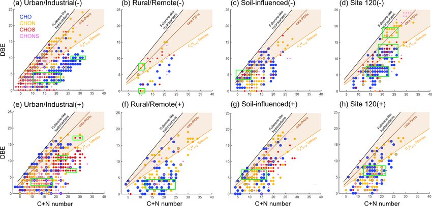
8532                    Y. Zhou et al.: Molecular composition, optical properties, and radiative effects of WSOC in snow

Earth’s land seasonally (Hall et al., 1995). Snowfall is a          tributed to organic chromophores. Subsequently, Beine et al.
crucial fresh water, nutrient, and carbon source for land           (2011) determined the light absorption of humic-like sub-
ecosystems (Jones, 1999; Mladenov et al., 2012), especially         stances (HULISs) in snow at Barrow, Alaska. They found
for barren regions such as northwestern China (Xu et al.,           that HULISs account for nearly half of the total absorption by
2010). Chemical deposits in the snowpack are highly pho-            dissolved chromophores within the photochemically active
tochemically and biologically active, which in turn influ-          wavelength region (300 to 450 nm), concluding that HULISs
ences biogeochemical cycles and the atmospheric environ-            are a major type of light absorber in Barrow snow and that
ment (Grannas et al., 2007; Liu et al., 2009). With respect         the HULIS-mediated photochemistry is probably important
to the climate effects, the snow–ice surface has the highest        for the regional environment. Several recent works have re-
albedo, which makes it the highest light reflecting surface         ported the radiative absorption of snow WSOC. Yan et al.
on Earth and a key factor influencing the Earth’s radiative         (2016) estimated the amount of the solar radiation absorbed
balance. The deposition of light-absorbing particles (LAPs),        by WSOC from snow collected in northern Tibetan Plateau
primarily black carbon (BC), organic carbon (OC), mineral           (TP), which was 10 % relative to that absorbed by BC, indi-
dust (MD), and microbes, on snow reduces the snow albedo            cating a non-negligible role of WSOC in accelerating snow
significantly and increases the absorption of solar radiation       and ice melting. Similar results were also reported for WSOC
(Hadley and Kirchstetter, 2012; Skiles et al., 2018). Conse-        extracted from other high-mountain areas (Niu et al., 2018;
quently, deposits of LAPs accelerate snow melting (Hansen           Zhang et al., 2019). However, chemical characterization and
and Nazarenko, 2004) and affect the snow photochemistry             optical properties of the light-absorbing WSOC (a.k.a. BrC)
(Zatko et al., 2013), further influencing the regional and          in the cryosphere are still an emerging topic. To date, no field
global climate (Bond et al., 2013; Flanner et al., 2007; Ja-        study has evaluated yet the composition-specific influence of
cobson, 2004). The albedo reduction and radiative forcing           WSOC on the snow albedo reduction.
(RF) due to the BC and MD deposits in snow have been a                 The fluorescence excitation–emission matrix (EEM) anal-
subject of many field studies (Doherty et al., 2010; Huang          ysis is a sensitive, rapid, and non-destructive optical spec-
et al., 2011; Pu et al., 2017; Shi et al., 2020; Wang et al.,       troscopy method (Birdwell and Valsaraj, 2010) that has been
2013, 2017b; Y. Zhang et al., 2018), remote sensing estimates       used to investigate the bulk composition and attribute po-
(Painter et al., 2010; Pu et al., 2019), and climate model sim-     tential sources of chromophoric WSOC in aquatic ecosys-
ulations (He et al., 2014; Qian et al., 2014; Zhao et al., 2014).   tems (Jaffé et al., 2014) and more recently in aerosols (Chen
Darkening of snow by biological organisms, like snow algae          et al., 2016b, 2020; Fu et al., 2015; Mladenov et al., 2011;
common in high-altitude and high-latitude snowpack, has             G. Wu et al., 2019). Based on parallel factor (PARAFAC)
also been investigated (Cook et al., 2017a, b; Ganey et al.,        analysis, contributions from main fluorescent components
2017; Lutz et al., 2014). However, yet little is known about        such as different fractions of HULIS and protein-like sub-
the chemical compositions, optical properties, and radiative        stances (PRLISs) can be quantitatively evaluated (Stedmon
effects of OC compounds in snow, which result from both de-         and Bro, 2008), indicating plausible sources of WSOC in
position of organic aerosol from natural and anthropogenic          aquatic (Murphy et al., 2008) and atmospheric samples (Wu
sources, as well as deposits of the wind-blown soil organic         et al., 2021). The chemical interpretations of PARAFAC-
matter (Pu et al., 2017; Wang et al., 2013).                        derived components are relatively well characterized for
    Water-soluble OC (WSOC) contributes to a large portion          aquatic WSOC, but it may not be simply applied to WSOC
(10 %–80 %) of organic aerosol (Kirillova et al., 2014; Y.-         in snow because their sources and geochemical processes are
L. Zhang et al., 2018), and it is also widely distributed in        highly different (Wu et al., 2021).
the cryosphere. The polar ice sheets and mountain glaciers             High-resolution mass spectrometry (HRMS) interfaced
store large amounts of organic carbon, which provide ap-            with soft electrospray ionization (ESI) can help to decipher
proximately 1.04 ± 0.18 Tg C yr−1 of WSOC exported into             the complexity of WSOC, providing an explicit description
proglacial aquatic environments (Hood et al., 2015), with a         of its individual molecular components (Qi et al., 2020).
substantial part of it being highly bioavailable (Singer et al.,    Thousands of individual organic species with unambiguously
2012; Y. Zhou et al., 2019b). WSOC components that ab-              identified elemental compositions can be detected at once by
sorb solar radiation at ultraviolet to visible (UV–vis) wave-       ESI–HRMS due to its high mass resolving power, mass ac-
lengths are collectively termed “brown carbon (BrC)” (An-           curacy, and dynamic range (Nizkorodov et al., 2011; Noziere
dreae and Gelencser, 2006) and have become the subject of           et al., 2015). Combined with a high-performance liquid chro-
many aerosol studies (Laskin et al., 2015). The optical prop-       matography (HPLC) separation stage and photodiode array
erties of WSOC in snow started to receive attention because         (PDA) detector, the integrated HPLC–PDA–HRMS platform
of its important role in initiating snow photochemistry (Mc-        enables the separation of WSOC components into fractions
Neill et al., 2012). Anastasio and Robles (2007) first quan-        with characteristic retention times, UV–vis spectra, and el-
tified the light absorption of water-soluble chromophores in        emental composition. Correlative analysis of these multi-
Arctic and Antarctic snow samples. They found that ∼ 50 %           modal data sets facilitates the comprehensive characteriza-
of absorption for wavelengths greater than 280 nm was at-           tion of chromophores present in complex environmental mix-

Atmos. Chem. Phys., 21, 8531–8555, 2021                                               https://doi.org/10.5194/acp-21-8531-2021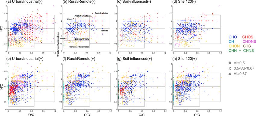
Y. Zhou et al.: Molecular composition, optical properties, and radiative effects of WSOC in snow                             8533

tures (Laskin et al., 2015; Lin et al., 2016, 2018; Wang et al.,   brown color were clearly seen on the filters following snow
2020a). Presently, HRMS studies of WSOC existing in the            water filtration (Fig. S1 in the Supplement), consistent with
cryosphere are still limited to the snow–ice in polar regions      the expected high loadings of soils at these sites. From the
(Antony et al., 2014, 2017; Bhatia et al., 2010) and moun-         R group, a sample from site 120 was considered separately
tain glaciers in the Alps (Singer et al., 2012) and on the         because it showed compositional and optical characteristics
TP (Feng et al., 2016; Spencer et al., 2014; L. Zhou et al.,       inconsistent with all other samples. For instance, it had very
2019) with perennial snowpack. For the regions mentioned           low BC concentration but the highest WSOC concentration
above, WSOC in snow–ice samples is dominated by protein-           among all the samples; hence, it is discussed separately.
or lipid-like compounds from autochthonous microbial ac-              Details of the sampling procedures can be found elsewhere
tivity with high bioavailability, whereas snow in northwest-       (Wang et al., 2013), and they are briefly described here. The
ern China is seasonal, the snowpack persists for 3–6 months        snow sampling sites were selected at least 20 km from cities
annually, and its composition is substantially influenced by       and villages and at least 1 km upwind of the approach road or
local soil dust and deposited aerosols from both natural and       railway such that the influence from single-point very local
anthropogenic sources (Pu et al., 2017). Therefore, the chem-      sources was minimized and the samples would rather reflect
ical compositions and optical properties of WSOC from this         conditions of large regional areas. The snow samples were
area snowpack are likely different from those reported for the     collected in sterile plastic bags (Whirl-Pak, Nasco, WI, USA)
remote regions with more persistent snow coverage.                 using clean, stainless steel utensils and by scooping ∼ 3 L of
   In this study, seasonal snow samples were collected across      snow from the top 5 cm at each site, resulting in ∼ 600 mL
the northern Xinjiang region of China in January 2018.             volume of melted snow water. For several sites with snow-
We investigate the optical and molecular characteristics of        pack deeper than 10 cm, subsurface snow (∼ 5–10 cm) was
WSOC using a range of analytical techniques, including UV–         also collected. Snow depths, snow density, and snow tem-
vis absorption spectrophotometry, EEM, and HPLC–ESI–               perature were also measured for each sampled snow layer
HRMS. Furthermore, based on the measured optical prop-             (Shi et al., 2020). All collected samples were then stored in a
erties and concentrations of snow impurities, as well as the       freezer (< −20 ◦ C) until further processing. A total of 28 sur-
physical properties of snow at each site, we calculate for the     face samples were analyzed by the following analytical tech-
first time extent of RF attributed to WSOC in snow.                niques.

                                                                   2.2   Chemical species analysis
2     Methods
                                                                   The snow samples were melted under room temperature and
2.1    Sample collection                                           immediately filtered by polytetrafluoroethylene (PTFE) sy-
                                                                   ringe filters with a pore size of 0.22 µm (Thermo Fisher, Inc.)
A total of 28 surface and 8 subsurface snow samples were           to remove insoluble solids. Obtained filtrates were then used
collected from 28 sites in Xinjiang, northwestern China, dur-      for the measurements of concentrations of soluble inorganic
ing a road trip in January 2018. The area map and sampling         ions, mass loadings of WSOC, acquisition of bulk UV–vis
locations are shown in Fig. 1a. The sampling sites were num-       absorption and EEM spectra, and molecular characterization
bered in chronological order and with a numbering scheme           using HPLC–ESI–HRMS platform.
adopted from our previous campaigns (Pu et al., 2017; Wang            The major inorganic ions (Na+ , NH+         +     2+
                                                                                                             4 , K , Mg , Ca ,
                                                                                                                               2+

et al., 2013, 2017b; Ye et al., 2012). The sampling sites were     Cl− , SO2−            −
                                                                             4 , and NO3 ) were measured by an ion chromatog-
classified into four groups based on their geographical lo-        raphy system (Dionex 600, Thermo Scientific, MA, USA)
cation and proximity to urban areas (Table S1 in the Sup-          using an IonPac AS22 column for anions and an IonPac
plement): urban/industrial (U) sites (nos. 106–118 and 131),       CS12A column for cations. The detection limits for all inor-
rural/remote (R) sites (nos. 119, 121–125, and 127–130),           ganic ions are greater than 0.05 mg L−1 . The concentrations
soil-influenced (S) sites (nos. 104, 105, and 126), and site       of WSOC were analyzed by a total organic carbon analyzer
120. The U sites were located north of the Tianshan Moun-          (Aurora 1030W, OI Analytical, TX, USA). Each measure-
tains, near major cities in Xinjiang area. These sites were        ment was done in triplicate, and the average concentrations
more likely influenced by local anthropogenic emissions (Pu        of four groups of samples and the values for each sample
et al., 2017). The rest of the sites were assigned to R group,     after blank subtraction are presented in Tables S2 and S3, re-
most of which were from desert areas or barren grasslands          spectively. The detection limit and relative standard deviation
located at least ∼ 50–100 km from major cities; hence, they        of measurements were 2 ppb and 1 %, respectively.
were mostly influenced by natural sources. The S sites are            The BC concentrations in snow were measured by a
a subgroup of the R group, and they correspond to specific         custom-developed two-sphere integration (TSI) spectropho-
locations where the snowpack was visibly patchy and shal-          tometer (Wang et al., 2020b) and have been reported by Shi
low, so local soil could be blown into snow by strong winds.       et al. (2020). The distribution of BC concentrations in snow
For the S samples, the coarse mineral particles of yellow-         samples is also shown in Fig. S2.

https://doi.org/10.5194/acp-21-8531-2021                                            Atmos. Chem. Phys., 21, 8531–8555, 2021
8534                     Y. Zhou et al.: Molecular composition, optical properties, and radiative effects of WSOC in snow

Figure 1. (a) Sampling locations and site numbers with photographs for typical land use types of sampling sites. (b) Spatial distribution of
WSOC concentrations in snow. Sampling sites are divided into four groups indicated by different colors. The bubble sizes are proportional to
the WSOC concentrations. (d) Variations in BC and WSOC concentrations among four groups of sites. The boxes denote the 25th and 75th
quantiles, the horizontal lines represent the medians, and the averages are shown as dots; the whiskers denote the maximum and minimum
data within 1.5 times the interquartile range, and the data points out of this range are marked with crosses (+).

2.3    UV–vis absorption and fluorescence EEM
       spectroscopic measurements                                                        ln(10) · A(λ)
                                                                        MACBrC (λ) =                   ,                                (1)
                                                                                          CWSOC · L
The UV–vis absorption and fluorescence EEM spectra were
recorded simultaneously by an Aqualog spectrofluorometer                where λ is the wavelength, A is the base-10 absorbance
(Horiba Scientific, NJ, USA) in a 1 cm quartz cuvette. The              measured by the spectrophotometer, CWSOC (mg L−1 ) is
excitation wavelengths for EEM were 240 to 600 nm in inter-             the concentration of WSOC, and L is the cuvette path
vals of 5 nm and were the same for UV–vis spectrum acquisi-             length (0.01 m). To characterize the wavelength dependence
tion. The fluorescence emission range was 250 to 825 nm in              of MACBrC , absorption Ångström exponents (AAEs) were
5 nm intervals with an integration time of 0.5 s. An ultrapure          determined by a power-law regression (Kirchstetter et al.,
water (18.2 M cm, Milli-Q purification system, Millipore,              2004):
Bedford, MA, USA) was used for blank measurement, sub-
tracted from all sample spectra.                                        MAC(λ) = k · λ−AAE ,                                            (2)
   The absorbance at 600 nm was subtracted from the whole
                                                                        where k is a constant related to WSOC concentrations. To
spectrum to correct the scattering effects and baseline shifts
                                                                        exclude absorption due to inorganic chromophores (e.g., ni-
of the instrument (Chen et al., 2019). The BrC mass absorp-
                                                                        trate), the AAE values were derived from the power law fits
tion coefficients (MAC; m2 g−1 ) related to WSOC contribu-
                                                                        limited to the range of 330–400 nm (AAE330−400 ) (Yan et al.,
tions were calculated by
                                                                        2016).

Atmos. Chem. Phys., 21, 8531–8555, 2021                                                    https://doi.org/10.5194/acp-21-8531-2021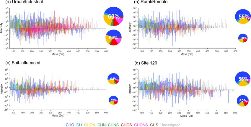
Y. Zhou et al.: Molecular composition, optical properties, and radiative effects of WSOC in snow                         8535

   Processing the EEM data followed the protocols described      Fisher Scientific Inc.). The elution protocol was 0–3 min hold
elsewhere (Y. Zhou et al., 2019a). Briefly, the raw EEM data     at 90 % A, 3–90 min linear gradient to 0 % A, 90–100 min
sets were first background subtracted to remove the water        hold at 0 % A, and then 100–130 min hold at 90 % A to re-
Raman scatter peaks, and then the inner filter effect was cor-   condition the column for the next sample. The column tem-
rected (Kothawala et al., 2013). The fluorescence intensi-       perature was maintained at 25 ◦ C, and the sample injection
ties were normalized to water Raman unit (RU) (Lawaetz           volume was 25 µL. The UV–vis absorption of eluted chro-
and Stedmon, 2009). The processed EEM data were ana-             mophores was recorded by a PDA detector over the wave-
lyzed by the PARAFAC model in a manner similar to our            length range of 200 to 680 nm. Correlation analysis between
previous report (Y. Zhou et al., 2019a). In this study, the      PDA and MS peaks and relative absorption of different chro-
PARAFAC modeling was conducted using the drEEM tool-             mophore fractions will be discussed in an upcoming paper.
box (version 0.2.0, http://models.life.ku.dk/drEEM, last ac-     For ESI–HRMS analysis, the following settings were used:
cess: 26 May 2021) (Murphy et al., 2013). According to           45 units of sheath gas, 10 units of auxiliary gas, 2 units of
the analysis of residual errors of two- to seven-component       sweep gas, a spray voltage of 3.5 kV, and a capillary temper-
models and split-half analysis, a three-component model          ature of 250 ◦ C, and a sweep cone was used. The mass spec-
was selected. Only two- and three-component models have          tra were acquired at a mass range of 80–1200 Da at mass re-
passed the split-half analysis with the “S4C6T3” split scheme    solving power of 1 m/m = 240 000 at m/z 200. Mass calibra-
(Fig. S3) (Murphy et al., 2013). Moreover, the sum of resid-     tion was performed using commercial calibration solutions
ual error decreased significantly when the number of com-        (PI-88323 and PI-88324, Thermo Scientific) for ESI(+/−)
ponents increased from two to three (Fig. S4). The spectra       modes.
of derived fluorescent components appeared consistent with          The raw experimental data files were acquired by Xcalibur
those commonly found in other studies (Table S4).                software (Thermo Scientific Inc.). The HPLC–ESI–HRMS
                                                                 data sets were preliminarily processed using an open-source
2.4   HPLC–ESI–HRMS molecular analysis and data                  software toolbox, MZmine 2 (http://mzmine.github.io/, last
      processing                                                 access: 26 May 2021), to perform peak deconvolution and
                                                                 chromatogram construction (Myers et al., 2017; Pluskal
The WSOC extracts were desalted and concentrated through         et al., 2010). The background subtraction and formula as-
solid phase extraction (SPE) method using DSC18 car-             signment were performed using customized Microsoft Ex-
tridges (Supelco, Millipore Sigma, PA, USA). The car-            cel macros (Roach et al., 2011). The formulas were assigned
tridges were conditioned and equilibrated by one-column          based on first- and second-order Kendrick mass defects and
volume (∼ 3 mL) of acetonitrile (ACN; Optima, LC/MS              a MIDAS formula calculator (https://nationalmaglab.org/
grade, Fisher Scientific Inc.) and one-column volume of wa-      user-facilities/icr/icr-software, last access: 26 May 2021).
ter (Optima, LC/MS grade, Fisher Scientific Inc.), respec-       [M + H]+ , [M + Na]+ , and [M−H]− ions were assumed to
tively. To increase the efficiency of SPE, the sample was        identify products detected in ESI+ and ESI− modes, respec-
acidified to pH ≈ 2 using HCl (Lin et al., 2010), and 3 mL       tively. Moreover, adduct ions were also identified and re-
of acidified sample flowed through the cartridge at a low flow   moved using a homemade MATLAB script (Text S2). The
rate of 1–2 drops per second. Salts and other unretained com-    molecular formulas were assigned using the following con-
pounds (e.g., small molecular acids and carbohydrates) were      straints: 1 ≤ C ≤ 50, 1 ≤ H ≤ 100, N ≤ 5, O ≤ 50, S ≤ 1,
first washed out by one-column volume of water, and the ana-     and Na ≤ 1 (ESI+ only) and mass tolerance of < 3.0 ppm.
lyte retained on the cartridge was then eluted by two-column     Furthermore, to eliminate the formulas not likely to be ob-
volumes of ACN. The efficiency of SPE was evaluated by           served in nature, the elemental ratio limits of 0.3 ≤ H/C ≤
measuring the UV–vis absorption before and after elution         3.0, 0.0 ≤ O/C ≤ 3.0, 0.0 ≤ N/C ≤ 1.3, 0.0 ≤ S/C ≤ 0.8
and ensured the good recovery of analytes (Sect. S1 in the       (Lin et al., 2012; Wang et al., 2018) were applied. The
Supplement). The ACN eluents were concentrated to 150 µL         double-bond equivalent (DBE) values of the neutral assigned
under a gentle stream of pure N2 and then diluted by adding      species Cc Hh Oo Nn Ss were calculated using the equation
150 µL of ultrapure water. Finally, the reconstituted extracts
were further concentrated to 200 µL prior to HPLC analysis.                   h n
                                                                 DBE = c −     + + 1.                                       (3)
   The obtained extracts were analyzed using a Vanquish                       2 2
HPLC system coupled to a Q Exactive HF-X Orbitrap HRMS              The aromaticity index (AI) is a conservative criterion for
with an Ion Max ESI source (all from Thermo Scientific           the unequivocal identification of aromatic and condensed
Inc.). The HPLC separation was performed on a Phenomenex         aromatic structures in natural organic matter calculated as
Luna C18 revised-phase column (2 mm × 150 mm, 5 µm par-          (Koch and Dittmar, 2006, 2016)
ticles, 100 Å pores). A gradient elution was performed at a
flow rate of 200 µL min−1 by an A + B binary mobile phase               1 + c − o − s − 0.5(h + n)
                                                                 AI =                              .                        (4)
system: (A) water with 0.05 % v/v formic acid and (B) ace-                     c−o−n−s
tonitrile with 0.05 % v/v formic acid (Optima, LC-MS grade,

https://doi.org/10.5194/acp-21-8531-2021                                          Atmos. Chem. Phys., 21, 8531–8555, 2021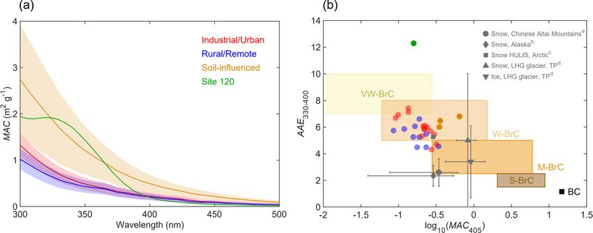
8536                     Y. Zhou et al.: Molecular composition, optical properties, and radiative effects of WSOC in snow

   AI > 0.5 and AI ≥ 0.67 are unambiguous minimum thresh-           Then, SSA, g, and extinction cross section (Qext ) were de-
olds for the presence of aromatic and condensed aromatic         rived from Mie code (https://omlc.org/software/mie/, last ac-
structures in a molecule, respectively. If either the numera-    cess: 26 May 2021), and the obtained values were then used
tor or denominator in Eq. (4) equals 0, then AI is assigned a    to calculate MEC (Seinfeld and Pandis, 2016):
value of 0.
   The intensity (I ∗ ) weighted molecular weight (MWw ) and               π d 2 /4 · Qext
                                                                 MEC =                     .                                (7)
other characteristic molecular parameters of H/C (H/Cw ),                   π d 3 /6 · ρ
O/C (O/Cw ), DBE (DBEw ), DBE/C (DBE/Cw ), and AI                   The spectral albedo (αλ ) was calculated for the scenarios
(AIw ) were calculated using Eq. (5):                            of pure snow and BC- and BrC-contaminated snow. After
       P ∗
          (Ii · Xi )                                             that, the broadband albedo (α) of each scenario needs to be
Xw =      P ∗ ,                                           (5)    determined to calculate the broadband albedo reduction (1α)
              Ii
                                                                 and RF due to different types of impurities; α was derived
where Xw represents any of the weighted parameters intro-        by integration of αλ over the wavelength range of 300 to
duced above, and Ii∗ and Xi are the corresponding intensity      1500 nm weighted by the incoming solar irradiance S(λ).
and the molecular parameter values calculated for each as-             R 1500
signed species i, respectively.                                               αλ S(λ)dλ
                                                                 α = 300R 1500                                             (8)
                                                                          300 S(λ)dλ
2.5    Snow albedo modeling and radiative forcing
       calculations                                                 The incoming solar irradiances were simulated by the cou-
                                                                 pled ocean–atmosphere radiative transfer (COART) model
The spectral snow albedo was calculated by the snow, ice,        (https://cloudsgate2.larc.nasa.gov/jin/coart.html, last access:
and aerosol radiative (SNICAR) model (Flanner et al., 2007),     26 May 2021) (Jin et al., 2006) for each site under clear sky
which accounts for the radiative transfer in the snowpack        assumptions; therefore, the calculated RF can be considered
based on the theory from Wiscombe and Warren (1980) and          as upper limits.
the two-stream, multilayer radiative approximation (Toon            The RF resulting from either BC or BrC in snow
et al., 1989). The input parameters required for the SNICAR      (RFBC,BrC ) was calculated by multiplying the downward
model are snow depth, snow density, effective snow grain         shortwave solar radiation flux at the surface by 1αBC,BrC
size, solar zenith angle, and impurity concentrations. Snow      (Painter et al., 2013):
depth and density were measured in the field. The effective
snow grain size was retrieved from the spectral albedo mea-      RFBC,BrC = E · 1αBC,BrC ,                                  (9)
sured in the field, and detailed information can be found in     1αBC,BrC = (αpure      snow − αBC,BrC ),                  (10)
our previous study (Shi et al., 2020). The solar zenith angle
was calculated using the site location and sampling date for     where E is the average daily downward shortwave so-
each site. The input values of parameters for the SNICAR         lar radiation flux acquired from NASA’s Clouds and
model, which are those for surface snow, are summarized in       the Earth’s Radiant Energy System (CERES) product
Table S5. For simplicity, a homogenous snowpack assump-          “CERES SYN1deg” (https://ceres.larc.nasa.gov/products.
tion was applied for both snow physical properties and pol-      php?product=SYN1deg, last access: 26 May 2021), and
lutant concentrations.                                           αpure snow and αBC,BrC are the broadband albedo of pure
   To evaluate the influence of BrC attributed to WSOC on        snow and BC or BrC contaminated snow, respectively.
the snow albedo, optical properties of BrC material such as
single scattering albedo (SSA), asymmetry factor (g), and        3     Results and discussions
mass extinction coefficient (MEC) are needed as inputs for
simulation. These parameters were calculated by Mie the-         3.1    Characteristics of chemical species
ory, approximating WSOC as an ensemble of small BrC par-
ticles distributed evenly in the snowpack. The input vari-       Figure 1b shows mass concentrations of WSOC measured in
ables required for Mie calculation are complex refractive in-    the snow samples, illustrating their broad range from 478 to
dex (RI = n − ik) and particle size parameter (x = π d/λ).       7069 ng g−1 with an average of 1775 ± 1424 ng g−1 (arith-
The diameter of individual particles (d), density (ρ), and the   metic mean ± 1 standard deviation, and same below). The U
real part (n) of RI of WSOC were assumed to be 150 nm,           and the S sites showed higher concentrations with averages
1.2 g cm−3 , and 1.55 (constant in the UV–vis range), respec-    of 1968 ± 953 and 2082 ± 1438 ng g−1 , respectively, while
tively (Chen and Bond, 2010; Z. Lu et al., 2015). The imagi-     the value of R sites (885 ± 328 ng g−1 ) was approximately
nary part (k) of RI was calculated as (Sun et al., 2007)         a factor of 2 lower (Table S2). Of note is that the WSOC
                                                                 concentrations in U and S samples reported here are signifi-
         MAC · ρ · λ
k(λ) =               .                                     (6)   cantly higher than those found in the snow and ice from po-
           4π                                                    lar regions (∼ 40–500 ng g−1 ) (Fellman et al., 2015; Hagler

Atmos. Chem. Phys., 21, 8531–8555, 2021                                              https://doi.org/10.5194/acp-21-8531-2021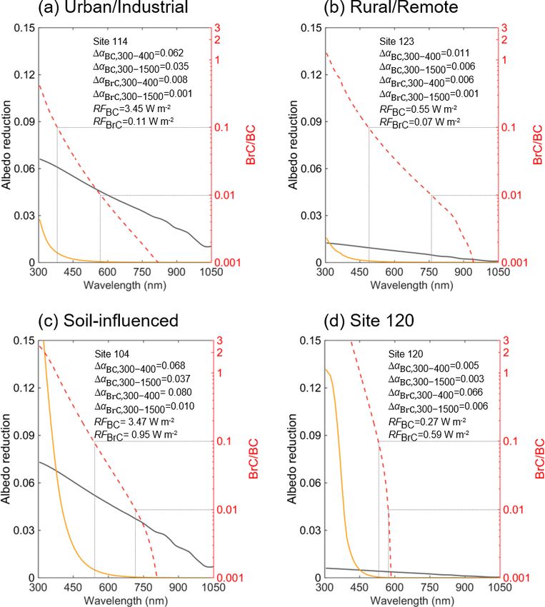
Y. Zhou et al.: Molecular composition, optical properties, and radiative effects of WSOC in snow                                      8537

Figure 2. (a) The average MAC spectrum of BrC attributed to WSOC in each group (solid lines, denoted by different colors); the shaded
areas represent one-time standard deviations. (b) Plot of the optical-based BrC classification scheme (Saleh, 2020) in the log10 (MAC405 )–
AAE330−400 space. The shaded areas represent very weakly absorbing BrC (VW-BrC), weakly absorbing BrC (W-BrC), moderately absorb-
ing BrC (M-BrC), and strongly absorbing BrC (S-BrC). BC is also shown for reference (Bond and Bergstrom, 2006). Grey marks indicate the
data from the literature for snow–ice samples from the Chinese Altai Mountains (a Zhang et al., 2019), Alaska (b Zhang et al., 2020), Arctic
(c Voisin et al., 2012; AAE is calculated for 300–400 nm), and LHG glacier on the TP (d Yan et al., 2016). Error bars denote the standard
deviations of AAE and MAC values.

et al., 2007a, b; Hood et al., 2015), glaciers in the European          than most of the values from high-altitude or high-latitude re-
Alps (∼ 100–300 ng g−1 ) (Legrand et al., 2013; Singer et al.,          gions of previous studies (∼ 40–700 ng g−1 as mentioned in
2012), and the remote TP region (∼ 150–700 ng g−1 ) (Yan                the last paragraph). It might be explained by two reasons:
et al., 2016). However, our reported WSOC mass concentra-               (1) there were more intensive anthropogenic emissions in the
tions are in the same range as those in the fresh snow samples          northern Xinjiang region, or (2) there was little snowfall dur-
collected from Laohugou (LHG) glacier, northern TP (2000–               ing 2018 campaign; therefore, WSOC had been potentially
2610 ng g−1 ) (Feng et al., 2018). It has been reported that            accumulated on the snow surface by sublimation and dry de-
glaciers and ice sheets from polar or alpine regions store a            position (Doherty et al., 2010). The sample from site 120 is
large amount of WSOC and discharge it to their downstream               discussed separately as it exhibited the highest WSOC con-
terrestrial ecosystems (Hood et al., 2009, 2015; Singer et al.,         centration (7069 ng g−1 ) and almost the lowest BC concen-
2012). Comparable or even higher concentrations of WSOC                 tration (44 ng g−1 ) out of all samples analyzed in this work.
in our samples indicate that the seasonal snow in northern              The potential sources of WSOC from the site 120 sample will
Xinjiang is also an important organic carbon source for the             be discussed in section 3.3.
terrestrial ecosystems during spring meltdown.
   As shown in Fig. 1c, the U sites were also associated                3.2    Bulk light-absorbing and fluorescence properties
with the highest BC concentrations among all four groups
(mean: 707 ± 651 ng g−1 ). Furthermore, the mass contribu-              The average MACBrC spectra of WSOC from differ-
tions of sulfate ions at U sites (Table S2; mean: 33 %± 7 %),           ent groups of samples are shown in Fig. 2a. The
which is a commonly used marker for fossil fuel burning                 average MACBrC at 365 nm (MAC365 ) of S samples
(Pu et al., 2017), were approximately twice as high as those            (0.94 ± 0.31 m2 g−1 ) was significantly higher than those of U
from the other sites. All these results indicate a strong influ-        (0.39 ± 0.11 m2 g−1 ) and R (0.38 ± 0.12 m2 g−1 ) samples
ence from anthropogenic pollution sources, explaining high              (Table S2). The information on MACBrC related to WSOC
WSOC loadings at U sites. For the S sites, HULISs from                  in snow and ice is yet very scarce in literature. The MAC365
local soil may dominate the WSOC composition. For exam-                 values of U and R samples are comparable to the re-
ple, snow at site 104 was patchy and thin (Fig. 1a, grass-              sults reported for continental snow collected across Alaska
land), and the local black soil can be lifted by winds and              (0.37 ± 0.32 m2 g−1 ) (Zhang et al., 2020) but slightly lower
then redeposited and mixed with snow. The assumption of                 than those for snow WSOC from the Chinese Altai Moun-
soil contributions agrees with the observed high mass con-              tains, which show a wide range from ∼ 0.3 m2 g−1 for ac-
tribution of calcium ions in S samples (mean: 50 %± 4 %,                cumulation season to ∼ 1.0 m2 g−1 for ablation season with
see Table S2). Although WSOC concentrations in R samples                an average of 0.45 ± 0.35 m2 g−1 (Zhang et al., 2019), and
were relatively low (885 ± 328 ng g−1 ), they were still higher         HULISs extracted from Arctic snow (∼ 0.5 m2 g−1 ) (Voisin
                                                                        et al., 2012). The snow–ice samples from LHG glacier on

https://doi.org/10.5194/acp-21-8531-2021                                                   Atmos. Chem. Phys., 21, 8531–8555, 2021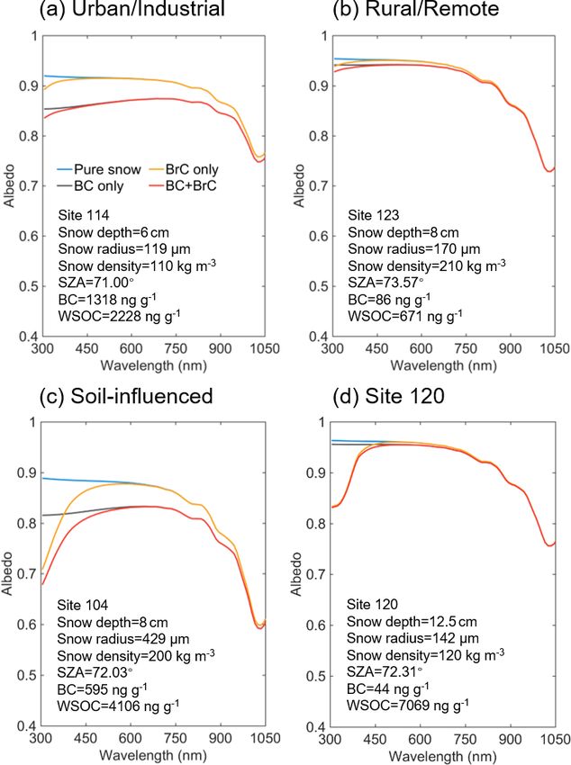
8538                    Y. Zhou et al.: Molecular composition, optical properties, and radiative effects of WSOC in snow

the TP (Yan et al., 2016) presented a higher average MAC365        cesses (Coble et al., 1998). Of note is that the fluorophores
(1.3–1.4 m2 g−1 ) than the S samples; they also indicated          detected in our samples show the similar peak positions com-
a large contribution of dust-derived organics. The relative        pared to the previous reports for aerosol or aquatic environ-
lower values of MAC365 measured for U samples might be             ments, but they do not necessarily have the same sources due
explained by photobleaching of WSOC during aging on the            to large differences in the physicochemical and geochemical
snow surface (Yan et al., 2016; Zhang et al., 2019). Due to        processes (Chen et al., 2016b; Duarte et al., 2007).
the stronger wavelength dependence of WSOC from U sam-                As shown in Fig. 3b and c, the relative intensities of
ples (AAE330−400 : 6.0 ± 0.8 vs. 5.4 ± 0.7 for U and R sites,      three fluorescent components were highly variable among
respectively), their MAC values at the shorter wavelength of       different groups of samples, suggesting systematic substan-
300 nm were higher compared to those of R samples. For             tial differences in their chemical compositions. HULIS-1
example, the averages of MAC300 were 1.32 ± 0.24 m2 g−1            dominates in the S samples, where it accounts for ∼ 49 %
and 1.02 ± 0.21 m2 g−1 for U and R samples, respectively           of the total fluorescence (Table S2). In addition, the rela-
(Table S2). The AAE330−400 values of our samples were in           tive intensities of HULIS-1 are positively correlated with
the range of 4.3 to 12.3 (mean: 6.0 ± 1.5), and S sites had        the mass fractions of calcium ions (r = 0.73, p < 0.01; Ta-
a higher average of 6.4 ± 0.3 than those corresponding to U        ble S6). These results suggest a terrestrial origin (soil dust)
and R samples. The highest AAE330−400 = 12. 3 was found            of HULIS-1, which is consistent with previous studies of wa-
for WSOC from the site 120 sample, and its UV–vis spectrum         ter systems and aerosols (Chen et al., 2016a, 2020; Sted-
also exhibited an unusual spectral shape with a well-defined       mon et al., 2003). A strongly negative correlation between
spectral feature observed between 300 and 350 nm. A simi-          the contributions of HULIS-1 and nitrate mass fractions is
lar feature was reported in (1) cryoconite samples collected       found as well (r = −0.68, p < 0.01), reflecting the poten-
from TP glaciers (Feng et al., 2016), which may be attributed      tially important role of HULIS in snow nitrate photochem-
to mycosporine-like amino acids (MAAs) produced by mi-             istry (Handley et al., 2007; Yang et al., 2018). For instance,
croorganisms (e.g., fungi, bacteria, and algae) (Elliott et al.,   Yang et al. (2018) found that HONO formation is signif-
2015; Shick and Dunlap, 2002), and (2) plant-derived (e.g.,        icantly enhanced in the presence of humic acid from ni-
corn, hairy vetch, or alfalfa) water-extractable organic matter    trate photolysis. HULIS-2 dominates U samples with an av-
containing phenolic carboxylic compounds (He et al., 2009).        erage contribution of ∼ 46 %. Given the significantly posi-
   Figure 2b shows MAC and AAE330−400 values measured              tive correlation between the contributions of HULIS-2 and
for BrC attributed to WSOC from our samples in the context         mass fractions of sulfate ions (r = 0.51, p < 0.01), the pri-
of an optical-based classification of BrC presented recently       mary relevance of anthropogenic emissions for HULIS-2 is
by Saleh (2020). The optical properties characterizing the         confirmed. The R samples show a significant contribution
BrC classes are expected to be associated with their corre-        of PRLIS fluorophore (mean: 48 %± 6 %), indicating an im-
sponding physicochemical properties (i.e., molecular sizes,        portant role of microbial processes in the composition of
volatility, and solubility). Most of our samples and HULIS         WSOC in these samples. This observation is in line with pre-
in Arctic snow (Voisin et al., 2012) fall into the region of       vious studies showing that snow is not only an active photo-
weakly absorbing BrC (W-BrC). The WSOC in snow–ice                 chemical site but also a biogeochemical reactor in the nitro-
from Alaska, the Chinese Altai Mountains, and LHG glacier          gen cycling (Amoroso et al., 2010). Amoroso et al. (2010)
was assigned to moderately absorbing BrC (M-BrC) but with          found that nitrate and nitrite ions in snow collected from Ny-
broader ranges, likely indicating higher molecular variability.    Ålesund, Norway, were most likely from microbial oxida-
These results provide a useful data set of snow BrC light-         tion of ammonium ions. Therefore, the significant correlation
absorbing properties which may inform climate models.              (r = 0.78, p < 0.01) between relative intensities of PRLIS
   Three fluorescent components (i.e., C1, C2, and C3) were        and nitrate mass fractions might be interpreted by (1) low
identified by PARAFAC analysis (Fig. 3a). The peak posi-           anthropogenic emissions and local soil dust import (fewer
tions of each component are summarized in Table S4. C1             contributions from sulfate and calcium ions) and (2) potential
(HULIS-1) is a type of terrestrial-derived humic fluorophore       metabolic production of nitrate/nitrite in snow at R sites. Fur-
with long emission wavelengths, commonly reported for              ther research is needed to investigate this hypothesis in more
samples of terrestrial aquatic systems and highly oxygenated       detail. Of interest, EEM from the site 120 sample cannot be
organic aerosols (Chen et al., 2016a; Stedmon et al., 2003).       modeled well by PARAFAC (Fig. S5) because of the un-
C2 (HULIS-2) is usually recognized as a HULIS from ma-             common spectroscopic feature with emission and excitation
rine sources (Coble, 1996) or phytoplankton degradation in         wavelengths of 315 and 452 nm, respectively. This feature
fresh water (Zhang et al., 2010), and it was also detected         is possibly attributed to (1) NADH-like (nicotinamide ade-
in anthropogenic wastewater (Stedmon and Markager, 2005)           nine dinucleotide) compounds, which are an indicator for the
and industrial-sourced aerosol (Chen et al., 2020). C3 is a        metabolism of organisms (Pöhlker et al., 2012), or (2) plant-
class of PRLIS (tyrosine-like) widely found in terrestrial or-     derived water-extractable organic matter (Hunt and Ohno,
ganics (Wu et al., 2020; Zhang et al., 2010; Zhao et al., 2016)    2007), e.g., corn. This result suggests strong influence from
related to labile organic matter produced from microbial pro-      either microbial activity or plant-sourced organics in snow at

Atmos. Chem. Phys., 21, 8531–8555, 2021                                              https://doi.org/10.5194/acp-21-8531-2021
Y. Zhou et al.: Molecular composition, optical properties, and radiative effects of WSOC in snow 8539
Figure 3. (a) The fingerprints of three fluorescent components identified by PARAFAC analysis. (b) Relative contributions of three compo-
nents to total fluorescence at each site. HULIS-1, HULIS-2, and PRLIS are represented in yellow, red, and blue, respectively. The size of
each pie is proportional to the total fluorescence intensity at each site. (c) The average contributions of three components in different groups
of samples.
site 120, which is also consistent with the UV–vis spectrum signed species from S samples was lowest (mean: 727 ± 146
shape. and 438 ± 84 for ESI+ and ESI− modes, respectively), re-
flecting the high molecular complexity of U samples. The
3.3 Molecular-level insights into composition of WSOC numbers of assigned formulas in this study are comparable to
from snow samples the assignments reported for urban aerosol samples (∼ 800–
1800) (Lin et al., 2012; Wang et al., 2017a) and WSOC of
3.3.1 General HRMS characteristics LHG glacier from the TP region (∼ 700–1900) (Feng et al.,
2016, 2018), but they are lower than those of WSOC from the
Numbers of assigned species ranged from 561 to 1487 Antarctic (∼ 1400–2600) and Greenland ice sheets (∼ 1200–
and from 339 to 1568 for ESI+ and ESI− modes, respec- 4400) (Antony et al., 2014; Bhatia et al., 2010).
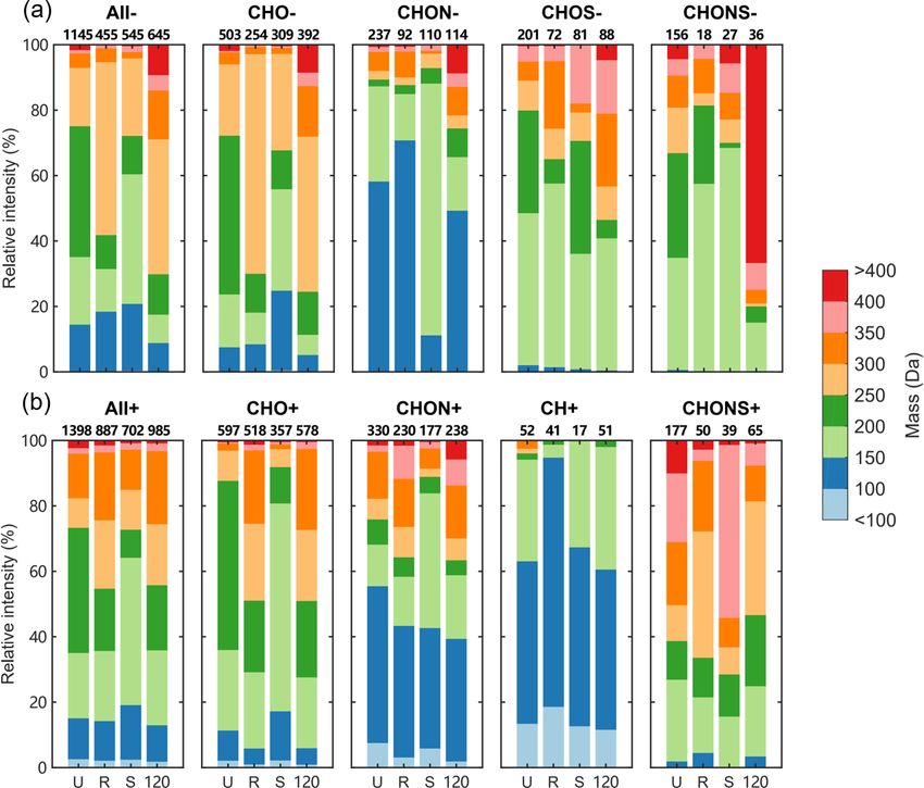
tively, suggesting high variations in molecular components of The mass spectrum plots constructed from individual sam-
WSOC in the snow samples from northern Xinjiang. The as- ples showing integrated composition of U, R, S, and site 120
signed peaks accounted for a majority (49 %–68 %) of all de- samples along with the corresponding number contributions
tected MS peaks. Due to the different ionization mechanisms from different formula categories are shown in Fig. 4. Over-
between positive and negative ESI (Lin et al., 2012), only all, the assigned formulas were mainly in the mass range of
small amounts of compounds were detected in both modes, 100 to 450 Da for both ESI+ and ESI−, while there were
accounting for approximately 15 % of total assignments at more compounds with masses lower than 100 in the ESI+
each representative site (Fig. S6). The assigned formulas mode. The relative intensities of MS features contributed by
were classified into eight categories, i.e., CHO, CHON, compounds in different mass ranges extract more informa-
CHOS, CHONS, CH, CHS, CHN, and CHS. CHONS re- tion from the mass spectra, as shown in Fig. 5. In ESI−
ferred to formulas containing carbon, hydrogen, oxygen, ni- mode, the ion intensity was most abundant in the mass range
trogen, and sulfur elements, and other categories were de- of 200 to 250 Da for U samples, 250 to 300 Da for R and
fined analogously. The U samples had the highest number site 120 samples, and 150 to 200 Da for S samples, indi-
of assigned compounds among four groups of sites in both cating different chemical constituents for samples from dif-
ESI+ and ESI− with averages of 1113 ± 203 and 871 ± 287, ferent groups. The variations in terms of relative intensities
respectively (Tables 1 and 2), whereas the number of as- for CHO− compounds were like those of all species de-
https://doi.org/10.5194/acp-21-8531-2021 Atmos. Chem. Phys., 21, 8531–8555, 20218540 Y. Zhou et al.: Molecular composition, optical properties, and radiative effects of WSOC in snow
Table 1. Averages (arithmetic mean ± standard deviation) of molecular characteristics in major formula categories detected in ESI+ mode
for each group of sites. Numbers and percentages of formulas and intensity-weighted MWw , H/Cw , O/Cw , DBEw , DBE/Cw , and AIw are
given.
All+ CH+ CHO+ CHON+ CHOS+ CHONS+ CHS+
U Number of formulas 1113 ± 203 48 ± 6 460 ± 68 249 ± 61 121 ± 33 135 ± 45 43 ± 15
Urban/industrial Percent of formulas (%) 4±1 42 ± 5 22 ± 1 11 ± 2 12 ± 2 4±1
(n = 14) Molecular weight (Da) 231 ± 9 146 ± 5 207 ± 21 211 ± 15 329 ± 18 294 ± 18 257 ± 13
H/Cw 1.51 ± 0.05 1.31 ± 0.04 1.72 ± 0.10 1.73 ± 0.14 1.12 ± 0.09 1.70 ± 0.08 1.11 ± 0.02
O/Cw 0.19 ± 0.04 0 0.28 ± 0.05 0.23 ± 0.02 0.07 ± 0.02 0.29 ± 0.04 0
DBEw 5.08 ± 0.60 4.6 ± 0.47 3.03 ± 0.66 3.68 ± 0.68 10.13 ± 0.70 4.10 ± 0.44 8.67 ± 0.63
DBE/Cw 0.34 ± 0.03 0.44 ± 0.02 0.24 ± 0.04 0.34 ± 0.07 0.49 ± 0.05 0.35 ± 0.04 0.51 ± 0.01
AIw 0.25 ± 0.04 0.44 ± 0.02 0.13 ± 0.03 0.17 ± 0.09 0.42 ± 0.07 0.15 ± 0.04 0.48 ± 0.01
R Number of formulas 942 ± 166 45 ± 11 533 ± 81 245 ± 51 25 ± 15 53 ± 13 7±3
Remote/rural Percent of formulas (%) 5±1 57 ± 2 26 ± 2 3±2 6±1 0.7 ± 0.2
(n = 10) Molecular weight (Da) 229 ± 10 134 ± 11 239 ± 12 214 ± 17 351 ± 21 260 ± 20 237 ± 30
H/Cw 1.69 ± 0.04 1.26 ± 0.08 1.75 ± 0.04 1.69 ± 0.10 1.51 ± 0.04 1.74 ± 0.08 1.17 ± 0.12
O/Cw 0.34 ± 0.01 0 0.39 ± 0.01 0.27 ± 0.02 0.10 ± 0.05 0.26 ± 0.02 0
DBEw 3.16 ± 0.21 4.53 ± 0.31 2.80 ± 0.16 4.11 ± 0.48 6.25 ± 0.51 3.92 ± 0.62 7.49 ± 1.64
DBE/Cw 0.26 ± 0.02 0.47 ± 0.04 0.22 ± 0.02 0.35 ± 0.05 0.30 ± 0.02 0.39 ± 0.03 0.49 ± 0.06
AIw 0.12 ± 0.03 0.47 ± 0.04 0.07 ± 0.03 0.18 ± 0.06 0.19 ± 0.03 0.15 ± 0.04 0.45 ± 0.07
S Number of formulas 727 ± 146 27 ± 11 407 ± 106 186 ± 39 34 ± 21 33 ± 4 7±6
Soil-influenced Percent of formulas (%) 4±1 56 ± 4 26 ± 0.3 5±3 5±1 1±1
(n = 3) Molecular weight (Da) 218 ± 15 138 ± 3 215 ± 30 188 ± 14 330 ± 11 290 ± 20 220 ± 32
H/Cw 1.73 ± 0.05 1.33 ± 0.02 1.84 ± 0.08 1.75 ± 0.06 1.35 ± 0.17 1.73 ± 0.06 0.92 ± 0.13
O/Cw 0.33 ± 0.04 0 0.40 ± 0.01 0.23 ± 0.01 0.07 ± 0.01 0.29 ± 0.05 0
DBEw 3.11 ± 0.45 4.29 ± 0.13 2.21 ± 0.53 3.31 ± 0.06 7.60 ± 1.56 4.23 ± 0.18 8.63 ± 0.34
DBE/Cw 0.25 ± 0.03 0.44 ± 0.01 0.18 ± 0.03 0.32 ± 0.03 0.38 ± 0.09 0.36 ± 0.02 0.61 ± 0.07
AIw 0.14 ± 0.05 0.44 ± 0.01 0.07 ± 0.02 0.15 ± 0.03 0.29 ± 0.09 0.13 ± 0.03 0.58 ± 0.07
Site 120 Number of formulas 987 51 578 238 10 65 4
(n = 1) Percent of formulas (%) 5 59 24 1 7 0.4
Molecular weight (Da) 234 145 245 212 338 246 250
H/Cw 1.69 1.29 1.72 1.80 1.54 1.95 1.14
O/Cw 0.32 0 0.37 0.26 0.06 0.29 0
DBEw 3.36 4.67 3.14 3.54 5.87 2.99 8.05
DBE/Cw 0.26 0.45 0.23 0.30 0.28 0.32 0.50
AIw 0.11 0.45 0.07 0.12 0.20 0.07 0.46
tected in ESI−. For CHON−, formulas with a mass of 150 to samples were significantly lower than those of the aged firn
200 Da were abundant in S samples, while other groups were and ice samples from the TP (∼ 40 %) (Feng et al., 2016,
dominated by formulas in the range of 100 to 150 Da. Sam- 2018, 2020; Spencer et al., 2014), which is mainly attributed
ple from site 120 showed higher fractions of formulas with to less microbial activities in our samples, but they were com-
masses larger than 300 Da, especially for CHONS− com- parable with those of fresh snow (Feng et al., 2018, 2020)
pounds. The distributions of all detected compounds showed in which the major source of WSOC is aerosol wet/dry de-
higher contributions from the mass range of 300 to 350 Da in position. These results indicate that WSOC from the snow-
ESI+ compared to ESI−. Although the detection of CH com- pack in northern Xinjiang was more likely from atmospheric
pounds in ESI is uncommon, some of them appear detectable aerosol depositions rather than from autochthonous sources.
in the ESI+ mode, and most were associated with aromatic There were much higher contributions of S-containing com-
species smaller than 150 Da (DBE ≥ 4). Furthermore, the pounds in the U samples, e.g., CHOS+ (11 %), CHONS+
CHONS+ species showed higher masses than CHONS−, (12 %), and CHS+ (4 %), which were less abundant in other
except for the sample from site 120. samples. These species showed low oxidation levels (mean
In ESI+ mode, CHO+ and CHON+ were the main com- O/Cw : 0.07 for CHOS+) and high unsaturation degree and
ponents in all samples, accounting for 35 % to 61 % and aromaticity (mean DBEw of 10.1 and 8.7 and mean AIw of
20 % to 28 % of total formulas, respectively (Table 1). The 0.42 and 0.48 for CHOS+ and CHS+, respectively), sug-
U samples showed the lowest CHO+ abundance (mean: gesting that they might be reduced S-containing species with
42 %± 5 %), while the sample from site 120 had the high- aromatic structures from incomplete fossil fuel combustion
est value (59 %). The fractions of CHON+ species in our (Mead et al., 2015; Wang et al., 2017a).
Atmos. Chem. Phys., 21, 8531–8555, 2021 https://doi.org/10.5194/acp-21-8531-2021Y. Zhou et al.: Molecular composition, optical properties, and radiative effects of WSOC in snow 8541
Table 2. Averages (arithmetic mean ± standard deviation) of molecular characteristics in major formula categories detected in ESI− mode
for each group of sites. Numbers and percentages of formulas and intensity-weighted MWw , H/Cw , O/Cw , DBEw , DBE/Cw , and AIw are
given.
All− CHO− CHON− CHOS− CHONS−
U Number of formulas 871 ± 287 404 ± 112 194 ± 79 156 ± 48 82 ± 49
Urban/industrial Percent of formulas (%) 47 ± 4 22 ± 2 18 ± 2 9±3
(n = 14) Molecular weight (Da) 223 ± 17 229 ± 19 183 ± 18 238 ± 17 252 ± 24
H/Cw 1.48 ± 0.09 1.57 ± 0.06 1.00 ± 0.14 1.68 ± 0.08 1.55 ± 0.15
O/Cw 0.35 ± 0.04 0.30 ± 0.05 0.45 ± 0.04 0.56 ± 0.05 0.60 ± 0.06
DBEw 4.14 ± 0.26 3.87 ± 0.31 5.59 ± 0.51 3.13 ± 0.42 4.55 ± 0.55
DBE/Cw 0.38 ± 0.06 0.30 ± 0.04 0.72 ± 0.08 0.29 ± 0.04 0.46 ± 0.08
AIw 0.19 ± 0.07 0.12 ± 0.04 0.54 ± 0.09 0.05 ± 0.02 0.14 ± 0.06
R Number of formulas 537 ± 92 266 ± 35 107 ± 21 100 ± 29 34 ± 16
Rural/remote Percent of formulas (%) 50 ± 4 20 ± 2 18 ± 2 6±2
(n = 10) Molecular weight (Da) 215 ± 21 216 ± 28 180 ± 12 241 ± 22 241 ± 27
H/Cw 1.44 ± 0.07 1.54 ± 0.10 1.03 ± 0.16 1.76 ± 0.10 1.52 ± 0.13
O/Cw 0.39 ± 0.06 0.37 ± 0.07 0.42 ± 0.04 0.58 ± 0.08 0.65 ± 0.07
DBEw 4.09 ± 0.31 3.70 ± 0.65 5.43 ± 0.69 2.68 ± 0.86 4.30 ± 0.79
DBE/Cw 0.42 ± 0.05 0.33 ± 0.05 0.72 ± 0.10 0.25 ± 0.06 0.49 ± 0.07
AIw 0.26 ± 0.05 0.13 ± 0.05 0.60 ± 0.14 0.04 ± 0.04 0.16 ± 0.06
S Number of formulas 438 ± 84 245 ± 53 85 ± 18 69 ± 9 22 ± 6
Soil-influenced Percent of formulas (%) 56 ± 2 19 ± 1 16 ± 2 5±1
(n = 3) Molecular weight (Da) 206 ± 3 195 ± 11 212 ± 27 249 ± 15 228 ± 11
H/Cw 1.53 ± 0.01 1.53 ± 0.01 1.48 ± 0.23 1.47 ± 0.22 1.76 ± 0.2
O/Cw 0.41 ± 0.02 0.42 ± 0.03 0.36 ± 0.02 0.42 ± 0.04 0.67 ± 0.03
DBEw 3.65 ± 0.07 3.40 ± 0.31 4.43 ± 1.51 4.51 ± 1.29 3.51 ± 0.32
DBE/Cw 0.36 ± 0.01 0.35 ± 0.00 0.43 ± 0.11 0.37 ± 0.12 0.38 ± 0.09
AIw 0.13 ± 0.01 0.12 ± 0.00 0.22 ± 0.10 0.09 ± 0.05 0.13 ± 0.05
Site 120 Number of formulas 645 392 114 88 36
(n = 1) Percent of formulas (%) 61 18 14 6
Molecular weight (Da) 280 286 212 271 396
H/Cw 1.41 1.46 0.99 1.51 1.15
O/Cw 0.34 0.32 0.48 0.50 0.44
DBEw 5.63 5.44 6.40 5.19 11.97
DBE/Cw 0.38 0.34 0.71 0.35 0.59
AIw 0.14 0.09 0.53 0.13 0.26
The abundance of CHO− was highest in ESI− with a WSOC in Xinjiang seasonal snow than those from remote
range of 41 % to 61 %. The U samples and the site 120 sam- areas.
ple showed the lowest (mean: 47 %± 4 %) and highest (61 %) The bulk molecular characteristics of compounds detected
fractions of CHO−. The CHON− and CHOS− compounds in ESI+ and ESI− are summarized in Tables 1 and 2, respec-
account for roughly equal contributions with ranges of 16 % tively. The MWw of all compounds detected in ESI+ mode
to 27 % and 14 % to 22 %, respectively. The detected CHOS was 231 ± 9, 229 ± 10, 218 ± 15, and 234 Da for U, R, S,
compounds were more abundant in ESI− than those in ESI+. and site 120 samples, respectively. These values are compa-
Furthermore, CHOS− compounds show a much higher ox- rable to the MWw of urban aerosols (∼ 225 to 265 Da) (Lin
idation level and lower unsaturation degrees than CHOS+ et al., 2012; Wang et al., 2018) but significantly lower than
(mean O/Cw of 0.55 and 0.08 and mean DBE of 3.2 and those of glacier samples (∼ 360 to 420 Da) (Feng et al., 2018,
8.3 for CHOS− and CHOS+, respectively). These results 2020), suggesting different compositions between WSOC
are consistent with previous ambient aerosol characteriza- in the seasonal snow of our study and from the literature-
tion studies (Lin et al., 2012; Wang et al., 2017a, 2018), but reported glacier samples. DBE is used to infer the unsatura-
the S-containing species were not abundantly detected in the tion degree of individual species (McLafferty et al., 1993),
glacier samples (Feng et al., 2016; Spencer et al., 2014), in- and AI is a more direct metric of their aromaticity (Koch and
dicating a stronger influence from anthropogenic aerosols to Dittmar, 2006, 2016). The U samples showed higher DBEw
https://doi.org/10.5194/acp-21-8531-2021 Atmos. Chem. Phys., 21, 8531–8555, 20218542 Y. Zhou et al.: Molecular composition, optical properties, and radiative effects of WSOC in snow
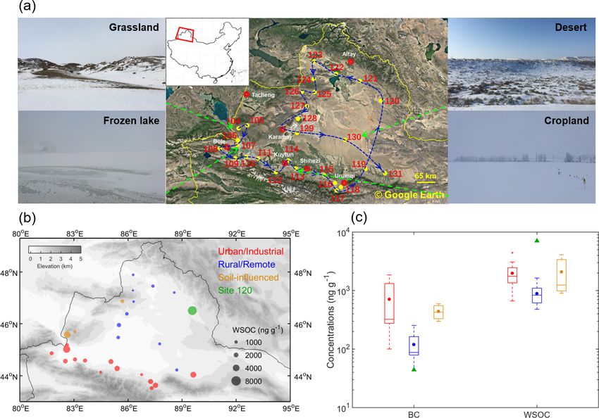
Figure 4. The reconstructed mass spectra of representative samples for four groups of sites: (a) site 114, (b) site 123, (c) site 104, and (d) site
120. The data measured by ESI+/− are plotted as positive/negative intensities, respectively. The pie charts show the number contributions
from different formula categories indicated by different colors, and the sizes of pie charts are proportional to the total numbers of assigned
formulas detected in each sample by ESI+/−. The percentages present the ratios of assigned formulas to total MS peaks. Unassigned peaks
were converted into neutral mass by assuming that they were protonated in ESI+ and deprotonated in ESI−.
and AIw values than the other groups of samples mainly 3.3.2 Chemical species in snow WSOC
due to high fractions of S-containing compounds in ESI+
mode (Table 1). As for ESI− mode, the MWw of the site 120
The Van Krevelen (VK) diagram is a frequently used
sample was higher than the other samples (280 vs. ∼ 200–
graphical method which plots the H/C ratios against the
220 Da). Of note is that the average MWw values of CHO−
O/C ratios in molecular formulas to qualitatively determine
and CHONS− compounds in the site 120 sample were 286
the major chemical species in complex organic mixtures
and 396 Da, respectively, which were approximately 70 and
and to explore their potential reaction pathways (Kim et al.,
150 Da higher than those from the other groups of samples.
2003). The VK diagrams of four representative samples
Accordingly, the DBEw of all formulas detected in the site
detected in ESI+ and ESI− modes are shown in Fig. 6. The
120 sample was the highest (5.8), and the values for CHO−
VK space in this study was separated into seven regions
and CHONS− were 5.4 and 12.0, respectively, which were
according to previous studies (Feng et al., 2016; Ohno
approximately 1.5 and 3 times higher than in the other sam-
et al., 2010): (1) lipid-like (O/C = 0–0.3, H/C = 1.5–2.0),
ples. These results indicate very unusual sources of WSOC
(2) aliphatic/protein-like (O/C = 0.3–0.67, H/C = 1.5–2.2),
in the site 120 sample. Additionally, the molecular charac-
(3) carbohydrate-like (O/C = 0.67–1.2; H/C = 1.5–2.4),
teristics of formulas detected in ESI− and ESI+ are differ-
(4) unsaturated hydrocarbons (O/C = 0–0.1, H/C = 0.7–
ent, e.g., higher average DBEw and AIw values of R samples
1.5), (5) lignins/carboxylic-rich alicyclic-molecule-like
for ESI− data (Tables 1 and 2). This results from the differ-
(CRAM) (O/C = 0.1–0.67, H/C = 0.7–1.5), (6) tannin-like
ences in ionization mechanisms between positive and neg-
(O/C = 0.67–1.2, H/C = 0.5–1.5), and (7) condensed aro-
ative modes. ESI+ is sensitive to protonatable compounds
matics (O/C = 0–0.67, H/C = 0.2–0.7). In ESI+, the U sam-
with basic functional groups, while acidic species are eas-
ples showed the lowest O/C ratios (mean: 0.19 ± 0.04) and
ily deprotonated and detected in ESI− mode (Cech and
H/C ratios (mean: 1.51 ± 0.05) among four groups (Table 1),
Enke, 2001). Therefore, using both positive and negative ESI
which indicates the low oxygenation and high unsaturation
modes provide a more complete molecular characterization
degree of WSOC from U samples, likely suggesting their
of WSOC.
primary emission sources (Kroll et al., 2011). Consequently,
the unsaturated hydrocarbons were most abundant among
seven classes of species (mean: 39 ± 15 %; Table 3), most of
Atmos. Chem. Phys., 21, 8531–8555, 2021 https://doi.org/10.5194/acp-21-8531-2021You can also read