SIMULATION OF FINE ORGANIC AEROSOLS IN THE WESTERN MEDITERRANEAN AREA DURING THE CHARMEX 2013 SUMMER CAMPAIGN - ATMOS. CHEM. PHYS
←
→
Page content transcription
If your browser does not render page correctly, please read the page content below
Atmos. Chem. Phys., 18, 7287–7312, 2018
https://doi.org/10.5194/acp-18-7287-2018
© Author(s) 2018. This work is distributed under
the Creative Commons Attribution 4.0 License.

Simulation of fine organic aerosols in the western Mediterranean
area during the ChArMEx 2013 summer campaign
Arineh Cholakian1,2 , Matthias Beekmann1 , Augustin Colette2 , Isabelle Coll1 , Guillaume Siour1 , Jean Sciare3,5 ,
Nicolas Marchand4 , Florian Couvidat2 , Jorge Pey4,a , Valerie Gros3 , Stéphane Sauvage6 , Vincent Michoud6,b ,
Karine Sellegri7 , Aurélie Colomb7 , Karine Sartelet8 , Helen Langley DeWitt4 , Miriam Elser9,c , André S. H. Prévot9 ,
Sonke Szidat10 , and François Dulac3
1 Laboratoire  Inter-Universitaire des Systèmes Atmosphériques (LISA), UMR CNRS 7583, Université Paris Est Créteil et
Université Paris Diderot, Institut Pierre Simon Laplace, Créteil, France
2 Institut National de l’Environnement Industriel et des Risques, Parc Technologique ALATA, Verneuil-en-Halatte, France
3 Laboratoire des Sciences du Climat et de l’Environnement, LSCE/IPSL, CEA-CNRS-UVSQ,

Université Paris-Saclay, Gif-sur-Yvette, France
4 Aix-Marseille Université, CNRS, LCE FRE 3416, Marseille, 13331, France
5 The Cyprus Institute, Energy, Environment and Water Research Center, Nicosia, Cyprus
6 IMT Lille Douai, Univ. Lille, Département Sciences de l’Atmosphère et Génie de l’Environnement, 59000 Lille, France
7 LAMP, Campus universitaire des Cezeaux, 4 Avenue Blaise Pascal, 63178 Aubière, France
8 CEREA, Joint Laboratory École des Ponts ParisTech – EDF R and D, Université Paris-Est, 77455 Marne la Vallée, France
9 Paul Scherrer Institute, 5232 Villigen – PSI, Switzerland
10 University of Bern, Freiestrasse 3, 3012 Bern, Switzerland
a now at: the Spanish Geological Survey, IGME, 50006 Zaragoza, Spain
b now at: Laboratoire Inter-Universitaire des Systèmes Atmosphériques (LISA), UMR CNRS 7583,

Université Paris Est, France
c now at: Laboratory for Advanced Analytical Technologies, Empa, Dübendorf, 8600, Switzerland

Correspondence: Arineh Cholakian (arineh.cholakian@lisa.u-pec.fr)

Received: 26 July 2017 – Discussion started: 23 October 2017
Revised: 6 March 2018 – Accepted: 21 April 2018 – Published: 25 May 2018

Abstract. The simulation of fine organic aerosols with            two parameterizations including aging of biogenic secondary
CTMs (chemistry–transport models) in the western Mediter-         OA, and a modified version of the VBS scheme which in-
ranean basin has not been studied until recently. The             cludes fragmentation and formation of nonvolatile OA. The
ChArMEx (the Chemistry-Aerosol Mediterranean Experi-              results from these four schemes are compared to observa-
ment) SOP 1b (Special Observation Period 1b) intensive field      tions at two stations in the western Mediterranean basin,
campaign in summer of 2013 gathered a large and compre-           located on Ersa, Cap Corse (Corsica, France), and at Cap
hensive data set of observations, allowing the study of differ-   Es Pinar (Mallorca, Spain). These observations include OA
ent aspects of the Mediterranean atmosphere including the         mass concentration, PMF (positive matrix factorization) re-
formation of organic aerosols (OAs) in 3-D models. In this        sults of different OA fractions, and 14 C observations showing
study, we used the CHIMERE CTM to perform simulations             the fossil or nonfossil origins of carbonaceous particles. Be-
for the duration of the SAFMED (Secondary Aerosol For-            cause of the complex orography of the Ersa site, an original
mation in the MEDiterranean) period (July to August 2013)         method for calculating an orographic representativeness er-
of this campaign. In particular, we evaluated four schemes        ror (ORE) has been developed. It is concluded that the modi-
for the simulation of OA, including the CHIMERE standard          fied VBS scheme is close to observations in all three aspects
scheme, the VBS (volatility basis set) standard scheme with       mentioned above; the standard VBS scheme without BSOA

Published by Copernicus Publications on behalf of the European Geosciences Union.
7288                           A. Cholakian et al.: Simulation of fine organic aerosols in the western Mediterranean area

(biogenic secondary organic aerosol) aging also has a sat-        or anthropogenic VOCs (volatile organic compounds) and
isfactory performance in simulating the mass concentration        SVOCs (semi-volatile organic compounds).
of OA, but not for the source origin analysis comparisons.           The chemical composition of aerosols has been studied
In addition, the OA sources over the western Mediterranean        in detail in the eastern Mediterranean area (Lelieveld et al.,
basin are explored. OA shows a major biogenic origin, es-         2002; Bardouki et al., 2003; Sciare et al., 2005, 2008; Koçak
pecially at several hundred meters height from the surface;       et al., 2007; Koulouri et al., 2008) and to a lesser extent in the
however over the Gulf of Genoa near the surface, the anthro-      western part (Sellegri et al., 2001; Querol et al., 2009; Min-
pogenic origin is of similar importance. A general assess-        guillón et al., 2011; Ripoll et al., 2014; Menut et al., 2015;
ment of other species was performed to evaluate the robust-       Arndt et al., 2017). Little focus has been given to the for-
ness of the simulations for this particular domain before eval-   mation of organic aerosol (OA) over the western Mediter-
uating OA simulation schemes. It is also shown that the Cap       ranean even if OA can play a significant role in both local
Corse site presents important orographic complexity, which        and global climate (Kanakidou et al., 2005) and can affect
makes comparison between model simulations and observa-           health (Pöschl, 2005; Mauderly and Chow, 2008). Its con-
tions difficult. A method was designed to estimate an oro-        tribution has been calculated in studies to be nearly 30 % in
graphic representativeness error for species measured at Ersa     PM1 for the eastern Mediterranean area during the FAME
and yields an uncertainty of between 50 and 85 % for primary      2008 campaign (i.e., Hildebrandt et al., 2010). It is also im-
pollutants, and around 2–10 % for secondary species.              portant to know the contribution of different sources (bio-
                                                                  genic, anthropogenic) to the total concentration of OA in the
                                                                  western part of the basin. Such studies have been performed
                                                                  for the eastern Mediterranean basin (e.g., Hildebrandt et al.,
1   Introduction                                                  2010), while for the western part of the basin, they have been
                                                                  in general restricted to coastal cities such as Marseilles and
The Mediterranean basin is subject to multiple emission           Barcelona (El Haddad et al., 2011; Mohr et al., 2012; Ripoll
sources; anthropogenic emissions that are transported from        et al., 2014).
adjacent continents or are produced within the basin, local or       The ChArMEx (the Chemistry Aerosol Mediterranean
continental biogenic and natural emissions among which the        Experiment; http://charmex.lsce.ipsl.fr, last access: 17 Au-
dust emissions from northern Africa can be considered as an       gust 2016) project was organized in this context, with a fo-
important source (Pey et al., 2013; Vincent et al., 2016). All    cus over the western Mediterranean basin during the period
these different sources, the geographic particularities of the    of 2012–2014, in order to better assess the sources, forma-
region favoring accumulation of pollutants (Gangoiti et al.,      tion, transformation, and mechanisms of transportation of
2001), and the prevailing meteorological conditions favor-        gases and aerosols. During this project, detailed measure-
able to intense photochemistry and thus secondary aerosol         ments were acquired not only for the chemical composition
formation, make the Mediterranean area a region experienc-        of aerosols but also for a large number of gaseous species
ing a heavy burden of aerosols (Monks et al., 2009; Nabat         from both ground-based and airborne platforms. The project
et al., 2012). In the densely populated coastal areas, this       ChArMEx is divided into different sub-projects, each with
aerosol burden constitutes a serious sanitary problem con-        a different goal; among those, the SAFMED (Secondary
sidering the harmful effects of fine aerosols on human health     Aerosol Formation in the MEDiterranean) project aimed
(Martinelli et al., 2013). In addition, studies have shown that   at understanding and characterizing the concentrations and
the Mediterranean area could be highly sensitive to future        properties of OA in the western Mediterranean (for exam-
climate change effects (Giorgi, 2006; Lionello and Giorgi,        ple Nicolas, 2013; Di Biagio et al., 2015; Chrit et al., 2017;
2007). This could affect aerosol formation processes, but in      Arndt et al., 2017; Freney et al., 2017). To reach these goals,
turn the aerosol load also affects regional climate (Nabat et     two intense ground-based and airborne campaigns were orga-
al., 2013). These interactions, the high aerosol burden in the    nized during July–August of 2013 and also summer of 2014.
area, and its health impact related to the high population den-   The focus of the present study is on the SAFMED campaign
sity situated around the basin make this region particularly      in summer of 2013, since detailed measurements on the for-
important to study.                                               mation of OA and precursors were obtained during this pe-
   The aforementioned primary emissions can be in the form        riod, namely at Ersa (Corsica) and Es Pinar (Mallorca). Other
of gaseous species, as particulate matter, or as semi-volatile    ChArMEx sub-projects and campaigns included the TRAQA
species distributed between both phases (Robinson et al.,         (Transport et Qualité de l’Air) campaign in summer 2012,
2007). In the atmosphere, they can subsequently undergo           set up to study the transport and impact of continental air on
complex chemical processes lowering their volatility, which       atmospheric pollution over the basin (Sič et al., 2016), and
leads to the formation of secondary particles. These pro-         the ADRIMED (Aerosol Direct Radiative Impact on the re-
cesses are not entirely elucidated especially for the formation   gional climate in the MEDiterranean, June–July 2013) cam-
of SOAs (secondary organic aerosols) for example (Kroll           paign aimed at understanding and assessing the radiative im-
and Seinfeld, 2008), starting from initially emitted biogenic     pact of various aerosol sources (Mallet et al., 2016).

Atmos. Chem. Phys., 18, 7287–7312, 2018                                             www.atmos-chem-phys.net/18/7287/2018/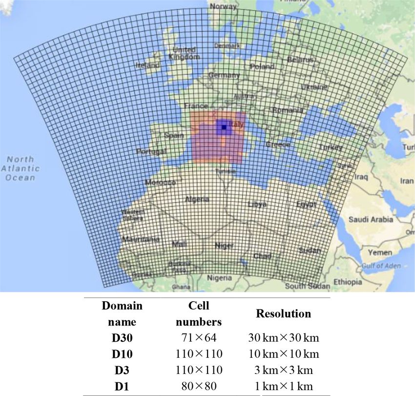
A. Cholakian et al.: Simulation of fine organic aerosols in the western Mediterranean area                                 7289

   Modeling of aerosol processes and properties is a difficult    in this section in more detail. The experimental data used for
task. Aside from the lack of knowledge of aerosol formation       simulation–observation comparisons are discussed in Sect. 3.
processes, the difficulty lies in the fact that OAs present an    An overall validation of the model is presented in Sect. 4,
amalgam of thousands of different species that cannot all be      together with comparisons of different gaseous and particu-
represented in a 3-D chemistry–transport model (CTM) due          late species and meteorological parameters to observations.
to limits in computational resources. Therefore a small num-      In Sect. 5, comparison of implemented schemes to measure-
ber of lumped species with characteristics that are thought to    ments regarding concentration, oxidation state, and origin
be representative of all the species in each group are used in-   of OA is presented. In Sect. 6, the contribution of different
stead. There are many different approaches that can be used       sources to the OA present in the whole basin is explored, be-
in creating representative groups for OAs (e.g., which char-      fore the conclusion in Sect. 7.
acteristics to use to group the species, which species to lump
together, physical processes that should be presented for their
simulation). It is therefore necessary to test these different    2   Model setup
simulation schemes for OAs in different regions and compare
the results to experimental data to check for their robustness.   The CHIMERE model (Menut et al., 2013; http://www.lmd.
For example, Chrit et al. (2017) modeled SOA formation in         polytechnique.fr/chimere, last access: 9 August 2016) is an
the western Mediterranean area during the ChArMEx sum-            offline regional CTM which has been tested rigorously for
mer campaigns, with a surrogate scheme that also contains         Europe and France (Zhang et al., 2013; Petetin et al., 2014;
ELVOCs (extremely low-volatility organic compounds). The          Colette et al., 2015; Menut et al., 2015; Rea et al., 2015).
simulated concentrations and properties (oxidation and affin-     It is also widely used in both research and forecasting ac-
ity with water) of OAs agree well with the observations per-      tivities in France, Europe, and other countries (Hodzic and
formed at Ersa (Corsica), after they had included the forma-      Jimenez, 2011). In this work, a slightly modified version of
tion of extremely low-volatility OAs and organic nitrate from     the CHIMERE 2014b configuration is used to perform the
monoterpene oxidation in the model.                               simulations. The modifications concern an updated descrip-
   The present study focuses on the comparison of differ-         tion of the changes in aerosol size distribution due to conden-
ent OA formation schemes implemented in the CHIMERE               sation and evaporation processes (Mailler et al., 2017). Four
chemistry–transport model for simulation of OA over the           domains are used in the simulations: a coarse domain cover-
western Mediterranean area. Different configurations of the       ing all of Europe and northern Africa with a 30 km resolu-
volatility basis set (VBS; Donahue et al., 2006; Robinson et      tion, and three nested domains inside the coarse domain with
al., 2007; Shrivastava et al., 2013) and the base parameteri-     resolutions of 10, 3, and 1 km (Fig. 1). The 10 km resolved
zation of the CHIMERE 3-D model (Bessagnet et al., 2008;          domain covers the western Mediterranean area and the two
Menut et al., 2013) are used for this purpose. Our work takes     smaller domains are centered on the Cap Corse, where the
advantage of the extensive experimental data pool obtained        main field observations in SAFMED were performed. Such
during the SAFMED campaign. This enables us to perform            highly resolved domains are necessary to resolve the com-
model–observation comparisons with unprecedented detail           plex orography of the Cap Corse ground-based measurement
over this region, including not only the OA concentration but     site, which will be discussed in Sect. 4, while for the flatter
also its origin (14 C analyses) and its oxidation state (posi-    Es Pinar site, a 10 km resolution is sufficient. The simula-
tive matrix factorization (PMF) method results). In addition,     tions for each domain contain 15 vertical levels starting from
a comparison for meteorological parameters and gaseous or         50 m to about 12 km above sea level (a.s.l.) with an average
particulate species which could affect the production of OA       vertical resolution of 400 m within the continental boundary
or could help analyze the robustness of the used schemes has      layer and 1 km above. The CHIMERE model needs a set of
been performed. Moreover, because of the orographic com-          gridded data as mandatory input: meteorological data, emis-
plexity of one of the sites (Ersa, Cap Corse) explored in this    sion data for both biogenic and anthropogenic sources, land
work, a novel method is designed to calculate the orographic      use parameters, boundary and limit conditions, and other op-
representativeness error of different species. To the best of     tional inputs such as dust and fire emissions. Given these in-
our knowledge, this is the first time that the concentrations     puts, the model produces the concentrations and deposition
of precursors, intermediary products, and OA concentrations       fluxes for major gaseous and particulate species and also in-
and properties have been simulated for different OA simu-         termediate compounds. The simulations presented in this ar-
lation schemes and compared for each scheme to multiple           ticle cover the period of 1 month from 10 July to 9 August.
series of measurements at different stations for the western         Meteorological inputs are calculated with the WRF
Mediterranean area. For OA schemes, the paper aims at as-         (Weather Research Forecast) regional model (Wang et al.,
sessing the robustness of each scheme with regard to differ-      2015) forced by NCEP (National Centers of Environmen-
ent criteria as mass, fossil, and modern fraction and volatil-    tal Predictions) reanalysis meteorological data (http://www.
ity. Section 2 describes the model and the inputs used for        ncep.noaa.gov, last access: 11 September 2016) with a base
the simulations. Also, the evaluated schemes are explained        resolution of 1◦ . Slightly larger versions of each domain with

www.atmos-chem-phys.net/18/7287/2018/                                              Atmos. Chem. Phys., 18, 7287–7312, 2018
7290                             A. Cholakian et al.: Simulation of fine organic aerosols in the western Mediterranean area

                                                                      for the year 2010 were used since this year was the latest
                                                                      common year in the two inventories.
                                                                         Biogenic emissions are calculated using MEGAN (Model
                                                                      of Emissions of Gases and Aerosols from Nature; Guen-
                                                                      ther et al., 2006) including isoprene, limonene, α-pinene, β-
                                                                      pinene, ocimene, and other monoterpenes with a base hori-
                                                                      zontal resolution of 0.008◦ × 0.008◦ . The land use data come
                                                                      from GlobCover (Arino et al., 2008) with a base resolution
                                                                      of 300 m × 300 m. Initial and boundary conditions of chem-
                                                                      ical species are taken from the climatological simulations
                                                                      of LMDz-INCA3 (Hauglustaine et al., 2014) for gaseous
                                                                      species and GOCART (Chin et al., 2002) for particulate mat-
                                                                      ter.
                                                                         The chemical mechanism used for the baseline gas-phase
                                                                      chemistry is the MELCHIOR2 scheme (Derognat et al.,
                                                                      2003). This mechanism has around 120 reactions to describe
                                                                      the whole gas-phase chemistry. The reaction rates used in
                                                                      MELCHIOR are constantly updated (last update in 2015);
                                                                      however, the reaction scheme itself has not been updated
                                                                      since 2003. Some reactions have been added to it by Bessag-
Figure 1. The four domains used in simulations (D30, D10, D3,         net et al. (2009) regarding the oxidation of OA precursors,
D1). The resolution for each domain is given in the table below the   but they do not affect gas-phase chemistry. Also, MEL-
image.                                                                CHIOR has been compared to SAPRC-07A, a more recent
                                                                      scheme (Carter, 2010), and the results show acceptable dif-
                                                                      ferences between the two schemes; for example, when com-
                                                                      pared to EEA (European Economic Area) ozone measure-
the same horizontal resolutions (Fig. 1) are used for the mete-       ments, both produce a correlation coefficient of 0.71. These
orological simulations. The WRF configuration used for this           comparisons are presented in Menut et al. (2013) and Mailler
study consists of the single-moment 5 class microphysics              et al. (2017).
scheme (Hong et al., 2004), the Rapid Radiative Transfer                 The CHIMERE aerosol module is responsible for the sim-
model (RRTMG) radiation scheme (Mlawer et al., 1997),                 ulation of physical and chemical processes that influence
the Monin–Obukhov surface layer scheme (Janjic, 2003),                the size distribution and chemical speciation of aerosols
and the NOAA Land Surface Model scheme for land sur-                  (Bessagnet et al., 2008). This module distributes aerosols in
face physics (Chen et al., 2001). Sea surface temperature up-         a number of size bins; here 10 bins range from 40 nm to
date, surface grid nudging (Liu et al., 2012; Bowden et al.,          40 µm, in a logarithmic sectional distribution, each bin span-
2012), ocean physics, and topographic wind options are ac-            ning over a size range of a factor of 2 (40–20, 20–10 µm,
tivated. Also, the feedback option is activated, meaning that         etc.). The module also addresses coagulation, nucleation,
the simulation of the nested domains can influence the par-           condensation, and dry and wet deposition processes. The ba-
ent domain. Some observation–simulation comparisons are               sic chemical speciation includes elemental carbon (EC), sul-
presented for meteorological parameters in Sect. 4.                   fate, nitrate, ammonium, SOA, dust, salt, and PPM (primary
   Anthropogenic emissions for all but shipping SNAP (Se-             particulate matter other than ones mentioned above).
lected Nomenclature for Air Pollution) sectors come from
the HTAP-V2 (Hemispheric Transport of Air Pollution;                  2.1     Organic aerosol simulation
http://edgar.jrc.ec.europa.eu/htap_v2/index.php, last access:
21 August 2016) inventory. The shipping sector in this in-            The SOA particles are divided, depending on their pre-
ventory was judged to overestimate ship traffic around the            cursors, into two groups: ASOA (anthropogenic SOA) and
Cap Corse area, especially on the shipping lines between              BSOA (biogenic SOA). Four schemes were tested to simu-
Marseilles and Corsica, due to overweighing ferries with re-          late their formation; more detail on each scheme is presented
spect to cargos (Van der Gon, personal communication). This           below.
could be explained by the fact that the boat traffic descrip-
tion is based on voluntary information. Therefore HTAP-V2             2.1.1    CHIMERE standard scheme
shipping emissions were replaced by those of the MACC-III
inventory (Kuenen et al., 2014). The base resolution of the           The SOA simulation scheme in CHIMERE (Bessagnet et al.,
HTAP inventory is 10 km × 10 km and that of the MACC-III              2008) consists of a single-step oxidation process in which
inventory is 7 km × 7 km. For both inventories the emissions          VOC lumped species are directly transformed into SVOCs

Atmos. Chem. Phys., 18, 7287–7312, 2018                                                www.atmos-chem-phys.net/18/7287/2018/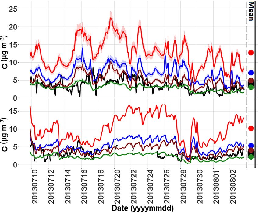
A. Cholakian et al.: Simulation of fine organic aerosols in the western Mediterranean area                                    7291

with yields that are taken from experimental data (Odum            can form aerosols. In total, the sum of 24 species in the model
et al., 1997; Griffin et al., 1999; Pun and Seigneur, 2007).       (with 10 size distribution bins each, i.e., 240 species in total)
These SVOC species are then distributed into gaseous and           makes up the total concentration of SOA simulated by this
particulate phases (Fig. 2a) following the partitioning theory     scheme.
of Pankow (Pankow, 1987). The precursors for this scheme
are presented in the Supplement (Sect. SI1). A number of           2.1.3   Modified VBS scheme
11 semi-volatile surrogate compounds are formed from these
precursors, which include six hydrophilic species, three hy-       The basic VBS scheme does not include fragmentation pro-
drophobic species, and two surrogates for isoprene oxidation.      cesses, corresponding to the breakup of oxidized OA com-
The sum of all 11 species results in the concentration of sim-     pounds in the atmosphere into smaller and thus more volatile
ulated SOA in this scheme.                                         molecules (Shrivastava et al., 2011). It also does not include
                                                                   the formation of nonvolatile SOA, where SOA can become
2.1.2   VBS scheme                                                 nonvolatile after formation (Shrivastava et al., 2015). In this
                                                                   work, these two processes were added to the VBS scheme
As an alternative to single-step schemes like the one in           presented above and tested for the Mediterranean basin. The
CHIMERE, the VBS approach was developed. In these types            volatility bins for the VBS model were not changed (ranges
of schemes, SVOCs are divided into volatility bins regard-         presented in the previous section). SOA yields were kept as
less of their chemical characteristics, but only depending         in the standard VBS scheme; however, instead of using the
on their saturation concentration. Therefore it becomes pos-       low-NOx or the high-NOx regimes, an interpolation between
sible to add aging processes in the simulation of OA by            the yields of these two regimes was added to the model. For
adding reactions that shift species from one volatility bin        this purpose, a parameter is added to the scheme, which cal-
to another (Donahue et al., 2006). This scheme was imple-          culates the ratio of the reaction rate of RO2 radicals with NO
mented and tested in CHIMERE for Mexico City (Hodzic               (high-NOx regime) with respect to the sum of reaction rates
and Jimenez, 2011) and the Paris region (Zhang et al., 2013).      of the reactions with HO2 and RO2 (low-NOx regime). For
The volatility profile used for this scheme consists of nine       this purpose, a parameter (α) is added to the scheme, which
volatility bins with saturation concentrations in the range of     calculates the ratio of the reaction rate of RO2 radicals with
0.01 to 106 µg m−3 (convertible to saturation pressure us-         NO (νNO ; high-NOx regime) with respect to the sum of reac-
ing atmospheric standard conditions), across which the emis-       tion rates of the reactions with HO2 (νHO2 ) and RO2 (νRO2 ;
sions of SVOCs and IVOCs are distributed, following a spe-         low-NOx regime). The parameter α is expressed as follows:
cific aggregation table (Robinson et al., 2007). Four volatil-                 νNO
                                                                   α=                     .                                     (1)
ity bins are used for ASOA and BSOA ranging from 1 to                   νNO + νHO2 + νRO2
1000 µg m−3 . SOA yields are taken from the literature (Lane
et al., 2008; Murphy and Pandis, 2009) using low-NOx con-            This α value represents the part of RO2 radicals reacting
ditions (VOC / NOx > 10 ppbC ppb−1 ). The SVOC species             with NO (which leads to applying “high NOx yields”). It is
can age, by decreasing their volatility by one bin indepen-        calculated for each grid cell by using the instantaneous NO,
dent of their origin with a given constant rate. SVOC species      HO2 , and RO2 concentrations in the model. Then, the fol-
are either directly emitted or formed from anthropogenic or        lowing equation is used to calculate an adjusted SOA yield
biogenic VOC precursors. Fragmentation processes and the           using this α value (Carlton et al., 2009).
production of nonvolatile SOAs are ignored in this scheme.         Y = α × YhighNOx + (1 − α) × YlowNOx                         (2)
In the basic VBS scheme, the BSOA aging processes are usu-
ally ignored since they tend to result in a significant overes-    The fragmentation processes for the SVOC start after the
timation of BSOA (Lane et al., 2008). Although physically          third generation of oxidation because fragmentation is fa-
present, their kinetic constants for this aging process are con-   vored with respect to functionalization for more oxidized
sidered the same as anthropogenic compounds and seem to            compounds. Therefore, three series of species in different
be overestimated. However, in Zhang et al. (2013), includ-         volatility bins were added to present each generation, similar
ing BSOA aging was necessary to explain the observed ex-           to the approach setup in Shrivastava et al. (2013). For bio-
perimental data. Therefore, in this work, the VBS scheme           genic VOC, fragmentation processes come into effect start-
is evaluated both with and without including the BSOA ag-          ing from the first generation, as in Shrivastava et al. (2013),
ing processes. Figure 2b shows a simplified illustration for       because the intermediate species are considered to be more
ASOA and BSOA, while the partition for SVOC is presented           oxidized. A fragmentation rate of 75 % (with 25 % left for
in the Supplement (Sect. SI2). For all bins, regardless of their   functionalization) is used in this work for each oxidation step
origin, the partitioning between gaseous and the particulate       following Shrivastava et al. (2015). The formation of non-
phases is performed following Raoult’s law and depends on          volatile SOA is performed by moving a part of each aerosol
total OA concentration. Under normal atmospheric condi-            bin to nonvolatile bins with a reaction constant correspond-
tions, SVOC with the volatility range of 0.01 to 103 µg m−3        ing to a lifetime of 1 h, similar to Shrivastava et al. (2015).

www.atmos-chem-phys.net/18/7287/2018/                                               Atmos. Chem. Phys., 18, 7287–7312, 2018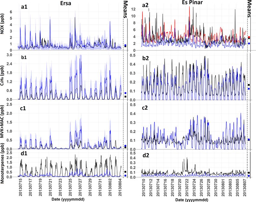
7292                              A. Cholakian et al.: Simulation of fine organic aerosols in the western Mediterranean area

Figure 2. Organic aerosol simulation schemes. (a) CHIMERE standard scheme (Bessagnet et al., 2008): from a parent volatile organic
compound (VOC), different semi-volatile organic compounds (SVOCs) (only one represented) are formed in a single step by oxidation; they
are in equilibrium between gas and aerosol phases (pSVOC); (b) VBS standard scheme (Robinson et al., 2007): from a parent VOC, SVOCs
with regularly spaced volatility ranges are formed and are in equilibrium with the aerosol phase. Aging of SVOC by functionalization is
included by passing species to classes with lower volatility; (c) modified VBS scheme (Shrivastava et al., 2015): here SVOC aging also
includes fragmentation, leading to transfer of species to classes with higher volatility. In addition, semi-volatile aerosol can be irreversibly
transformed into nonvolatile aerosol (yellow-filled circle). For each bin, saturation concentration is shown in micrograms per cubic meter.
Note that this schematic represents BSOA and ASOA (biogenic and anthropogenic secondary organic aerosol) where four bins are used;
for SVOC and IVOC (semi-volatile and intermediate-volatility organic compounds, where nine bins are used) a schematic is presented in
Supplement Sect. SI1.

Figure 2c shows a scheme of the modified VBS for the VOC.                 ments carried out in this station are reported in Table 1. More
In total, 40 species (with 10 size distribution bins each, i.e.,          details about the instrumental setup in Ersa can be found in
400 species in total) are added together to calculate the total           Michoud et al. (2017) and Arndt et al. (2017).
concentration of SOA simulated by this scheme. The result-                   The Es Pinar supersite (39◦ 530 04.600 , 3◦ 110 40.900 ) is lo-
ing model has a total of 740 species in the output files (in-             cated on the northeastern part of Mallorca. The monitoring
cluding gas-phase chemistry), which makes this scheme the                 station was placed in the “Es Pinar” military facilities be-
most time consuming among the tested schemes. In Sect. 5                  longing to the Spanish Ministry of Defense. The environ-
of this paper, the results from the three schemes introduced              ment is a non-urbanized area surrounded by pine forested
above will be compared to observations.                                   slopes and is one of the most insulated zones on Mallorca,
                                                                          in between the Alcúdia and Pollença bays, but can still be
                                                                          influenced by local anthropogenic emissions. The site is lo-
3     Experimental data set                                               cated at an altitude of 20 m a.s.l. The location of the station
                                                                          and a list of available measurements are presented in Fig. 3
During the SAFMED sub-project, measurements were made                     and Table 1, respectively.
at two major sites, the Ersa, Cap Corse, station and the Cap                 At Ersa, NOx (nitrogen oxides) were measured using a
Es Pinar, Mallorca, station. The geographical characteristics             CraNOx analyzer using ozone chemiluminescence with a
and the measurements performed at each site are presented                 resolution of 5 min. The photolytic converter in the ana-
in the following section.                                                 lyzer allows the conversion of direct measurements of NO2
                                                                          into NO in a selective way, thus avoiding interferences with
3.1    ChArMEx measurements                                               other NOy species. At Es Pinar, an API Teledyne T200 with
                                                                          molybdenum converter was used; therefore, the measure-
The Ersa supersite (42◦ 580 04.100 , 9◦ 220 49.100 ) is located on
                                                                          ments are not specific to NO2 and interferences of NOy
the northern edge of Corsica, in a rural environment, at an
                                                                          are possible for these measurements. VOCs were moni-
altitude of 530 m a.s.l. The station is located on a crest that
                                                                          tored at both supersites using a proton-transfer-reaction time-
dominates the northern part of the cape. It has a direct view of
                                                                          of-flight mass spectrometer (PTR-ToF-MS) (Kore™ second
the sea on the western, northern, and eastern sides. Measure-

Atmos. Chem. Phys., 18, 7287–7312, 2018                                                      www.atmos-chem-phys.net/18/7287/2018/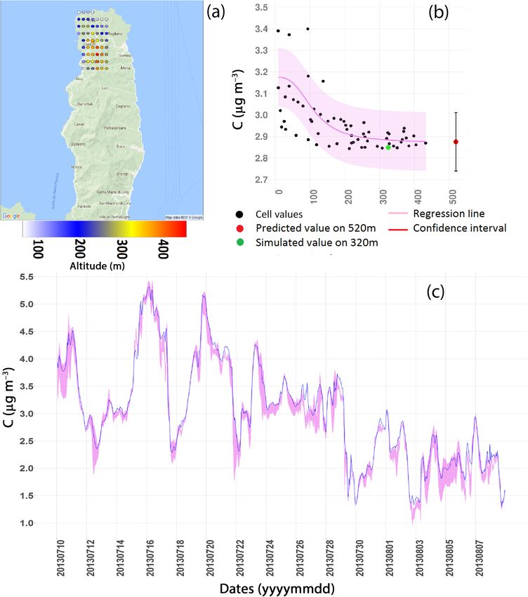
A. Cholakian et al.: Simulation of fine organic aerosols in the western Mediterranean area 7293
Table 1. Gas and aerosol and meteorological measurements used for this study.
(1) Ersa, France (42◦ 580 04.100 , 9◦ 220 49.100 )
Gases: NOx (CRANOX), VOCs (PTR-ToF-MS-KORE)
Aerosols: PM10 total mass (TEOM-FDMS), online (non-refractive) PM1
Chemistry : OA, SO2− + − 14
4 , NH4 , NO3 (ACSM), C (PM1 , daily filters),
BC (PM2.5 , MAAP)
Meteorology: temperature, wind speed, wind direction, relative humidity
(2) Es Pinar, Spain (39◦ 530 04.600 , 3◦ 110 40.900 )
Gases: NOx (API Teledyne T200), VOCs (PTR-ToF-MS, Ionikon)
Aerosols: PM10 total mass (BETA corrected by factor obtained after
comparison with gravimetric), PM1 online Chemistry: OA, SO2− 4 ,
NH+ − 14
3 , NO3 (HR-ToF-AMS), C (PM1 , daily filters),
BC (PM2.5 , Aethalometer AE33)
Meteorology: temperature, wind speed, wind direction, relative humidity
(3) Palma, Spain (39◦ 360 20.8800 , 2◦ 420 23.759400 ), (4) Nîmes, France (43◦ 510 21.600 , 4◦
240 21.599400 ), (5) Ajaccio, France (41◦ 550 5.325600 , 8◦ 470 38.053800 )
Radiosondes: T , RH, wind speed, wind direction; at 00:00 and 12:00 UTC each day
A quadruple aerosol chemical speciation monitor (Q-
ACSM, Aerodyne Research Inc.; Ng et al., 2011) was used
for the measurements of the chemical composition of non-
refractory submicron aerosol at Ersa with a time resolution
of 30 min. This instrument has the same general structure
of an AMS (aerosol mass spectrometer), with the differ-
ence that it was developed specifically for long-term monitor-
ing. A high-resolution time-of-flight AMS (HR-ToF-AMS,
Aerodyne Research Inc.; Decarlo et al., 2006) operated un-
der standard conditions (i.e., temperature of the vaporizer
set at 600 ◦ C, electronic ionization (EI) at 70 eV) was de-
ployed with a temporal resolution of 8 min to determine
the bulk chemical composition of the non-refractory frac-
tion of the aerosol for the Es Pinar site. AMS data were pro-
cessed and analyzed using the HR-ToF-AMS analysis soft-
ware SQUIRREL (SeQUential Igor data RetRiEvaL) v.1.52L
and PIKA (Peak Integration by Key Analysis) v.1.11L for
the IGOR Pro software package (Wavemetrics, Inc., Port-
land, OR, USA). Q-ACSM and AMS source apportionment
results discussed in this work are detailed in Michoud et
al. (2017). For both sites, source contributions were obtained
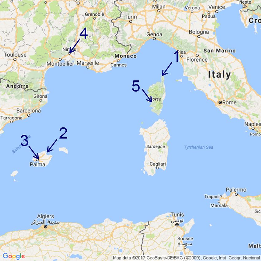
Figure 3. Experimental data sites, including in situ surface stations from PMF analysis (Paatero and Tapper, 1994) of Q-ACSM
(1: Ersa, France; 2: Cap Es Pinar, Spain) and meteorological sound- and AMS OA mass spectra. PMF was solved using the multi-
ing stations (3: Palma, Spain; 4: Nîmes, France; 5: Ajaccio, France). linear engine algorithm (ME-2; Paatero, 1997), using the
More details about exact location and measurements performed can Source Finder toolkit (SoFi; Canonaco et al., 2013). For
be found in Table 1. the Ersa site, the HOA (hydrocarbon-like organic aerosol)
profile was constrained with a reference HOA factor us-
ing an a value of 0.1. The a value refers to the extent to
generation at Ersa, and Ionikon™ PTR-ToF-MS 8000 at Es which the output HOA factor is allowed to vary from the
Pinar). A detailed procedure of VOC quantification is pro- input HOA reference mass spectra (i.e., 10 % in this case;
vided in Michoud et al. (2017) for Ersa. Briefly, both in- Canonaco et al., 2013). In such a remote environment, the
struments were calibrated daily using gas standard calibra- HOA factor could not be extracted from the OA mass spec-
tion bottles and blanks performed by means of a catalytic tral matrix with a classic unconstrained PMF approach. Two
converter (stainless steel tubing filled with Pt wool held at other factors were extracted, without any constrains, includ-
350 ◦ C).
www.atmos-chem-phys.net/18/7287/2018/ Atmos. Chem. Phys., 18, 7287–7312, 2018
7294                             A. Cholakian et al.: Simulation of fine organic aerosols in the western Mediterranean area

ing SVOOA (semi-volatile oxygenated organic aerosol) and              4     Model validation
LVOOA (low-volatility oxygenated organic aerosol). For the
Es Pinar site, HOA has been constrained using an a value              The CHIMERE model has been previously validated for dif-
of 0.05. Three additional factors were retrieved, including an        ferent parts of the world (Hodzic and Jimenez, 2011; Solazzo
SVOOA and two LVOOA factors. In addition to HOA, three                et al., 2012; Borrego et al., 2013; Berezin et al., 2013; Pe-
other factors have been extracted from the PMF analysis: one          tetin et al., 2014; Rea et al., 2015; Konovalov et al., 2015;
SVOOA and two LVOOA factors. Differences between these                Mallet et al., 2016). The data set presented in Sect. 3 is used
two LVOOA factors are mainly linked to air mass origins               for model validation. First, a representativeness error within
and to the probable influence of marine emissions. For the            simulations is calculated for a list of pollutants, which is nec-
marine LVOOA factor at both sites, a correlation coefficient          essary to distinguish between uncertainties due to limitations
(R 2 ) of 0.43 and 0.47 with the main fragment derived from           in model resolution and due to other reasons. Then a vali-
methane sulfonic acid (MSA, fragment CH3 SO+     2 ) was found        dation for the meteorological parameters is presented, before
for Es Pinar and Ersa, respectively. For the sake of clarity          comparison of simulation results to gaseous and aerosol mea-
and for the purpose of intercomparison with the model out-            surements.
comes, we merge the two LVOOA factors into one LVOOA
for the Cap Es Pinar site to be compared to the Ersa site re-         4.1    Orographic representativeness of Cap Corse
sults. Online aerosol chemical characterization was comple-                  simulations
mented by an Aethalometer (AE33, MAGEE; Drinovec et
al., 2015) at Es Pinar and a multiangle absorption photome-           As explained before, during the ChArMEx campaign, an
ter (MAAP5012, Thermo) for the quantification of black car-           important number of observations were made at Ersa, Cap
bon (BC) at Ersa. PM10 total mass measurements were taken             Corse. In order to use this data set for model evaluation,
from TEOM-FDMS (tapered element oscillating microbal-                 potential discrepancies due to a crude representation of the
ance filter dynamic measurement system) at Es Pinar and cor-          complex orography of Cap Corse need to be minimized and
rected by a factor obtained after comparison to gravimetric           quantified since the measurements were performed on the
measurements. Finally, daily PM1 aerosol samples were col-            crest line.
lected onto 150 mm quartz fiber filters (Tissuquartz, Pall) at           For the 10 km domain (D10), we noticed that there was
both sites. A total of 18 and 8 samples were selected for Ersa        an inconsistency between simulated and real altitude of the
and Es Pinar, respectively, for a subsequent analysis of radio-       cell where the Ersa site is located, altitude being simu-
carbon performed on both organic carbon (OC) and EC frac-             lated at 360 m a.s.l. below the real altitude of measurements
tions following the method developed in Zhang et al. (2012).          (530 m a.s.l.). Therefore, 1 km horizontally resolved simula-
                                                                      tions were performed for the inner domain. However, even
3.2    Other measurements                                             for the 1 km simulations the simulated altitude remains too
                                                                      low (365 m a.s.l.). This error occurs because the altitude of
For the validation of meteorological parameters, along                each cell in CHIMERE is calculated using the average of al-
with the meteorological surface measurements performed                titudes of points inside the cell; therefore if the altitude of
at ChArMEx stations, radiosonde data for three stations in            the ground surface inside a cell happens to vary greatly, the
the western Mediterranean basin were used for simulation–             average would be lower than the higher points seen in the
observation comparisons for meteorological parameters. The            cell (which corresponds in our case to the Ersa site located
radiosondes are performed by Météo France at the two sta-             on the crest). In addition, the average of the marine boundary
tions of Ajaccio, France (41◦ 550 500 , 8◦ 470 3800 ), and Nîmes,     layer height is typically around 500 m (Stull, 1988); there-
France (43◦ 510 2200 , 4◦ 240 2200 ), and by AEMet at Palma,          fore a discrepancy in the simulated altitude could cause sig-
Spain (39◦ 360 2100 , 2◦ 420 2400 ). Each day two balloons at about   nificant errors in the simulations. These two reasons make it
00:00 and 12:00 UTC are available for each station; a total           important to explore the representativeness of the simulations
of 96 balloons are included in the comparisons. Ajaccio and           regarding this station.
Palma are coastal stations, but Nîmes is farther from the coast          This led us to perform an orographic representativeness
compared to the other two stations. Each day two balloons             test on the 1 km domain (D1) at the Ersa site. A matrix of
were launched at about 00:00 and 12:00 UTC at each station,           neighboring cells around the grid cell covering the Ersa sta-
and a total of 96 balloons are included in the comparisons for        tion (up to 5 km distance) was taken (Fig. 4a), and species
an altitude between the surface and 10 km.                            concentrations were plotted against the variation of the alti-
                                                                      tude of these different cells. The highest altitude reached by
                                                                      one of the cells is about 450 m. Then, the concentration on
                                                                      the exact altitude (530 m) was extrapolated using a nonlinear
                                                                      regression between the altitude and the concentration of the
                                                                      selected cells with several different equations for each time
                                                                      step. In total, nine nonlinear equations were tested, among

Atmos. Chem. Phys., 18, 7287–7312, 2018                                                www.atmos-chem-phys.net/18/7287/2018/
A. Cholakian et al.: Simulation of fine organic aerosols in the western Mediterranean area                                              7295

Figure 4. Orographic representativeness error. (a) Neighboring cells used in the orographic representativeness test; (b) an example of non-
linear regressions performed on one time step for organic aerosol (OA, one point corresponds to one grid cell); (c) results from all hourly
simulations for OA. In (b) and (c), the purple ribbon shows the confidence interval of the regression results. In (c), the blue line shows the
simulations at the nominal Ersa site grid cell.

which only five were finally used for the calculation of the             verging regressions were not retained for a given time step,
representativeness error. For the other four equations, con-             the results for that time step were not further used. Figure 4c
vergence problems occurred and no stable solution could be               shows the compiled results for all equations and all simu-
found for some of the hourly time steps (see Supplement                  lation times in one time series for total OA concentration.
Sect. SI3 for details). Regressions were performed separately            Note that model output was generated with an hourly time
for each of the 720 hourly time steps of the 1-month simula-             step. Using these results, for a list of different species, an
tions. An example of this regression for OAs for one time                orographic representativeness error was calculated using the
step and one of the equations is shown in Fig. 4b (Eq. 1                 average of the difference of the upper and lower confidence
from SI3). The results were filtered using two criteria (con-            intervals for all equations. As an example, carbon monoxide,
vergence of regression for each time step and a correlation              which is a well-mixed and a more stable component in the at-
coefficient between fitted and simulated points of higher than           mosphere, presents the lowest error among the tested species
a threshold) depending on statistical values of the regressions          (2 %). Ozone also presents one of the lowest errors (4 %) and
(see Supplement Sect. SI3 for details) and only regressions              nitrogen oxides one of the highest (75 %). OA, of particu-
conforming to these criteria were retained. If at least two con-         lar interest for this study, shows a moderate error of 10 %.

www.atmos-chem-phys.net/18/7287/2018/                                                       Atmos. Chem. Phys., 18, 7287–7312, 2018
7296                            A. Cholakian et al.: Simulation of fine organic aerosols in the western Mediterranean area

In terms of meteorological parameters, relative humidity ap-        cio. Wind speed shows a good correlation at higher altitudes,
pears more affected (relative orographic representativeness         and also near the surface for Nîmes and Palma for radiosonde
error of 18 %) than temperature (the relative orographic rep-       stations, while for the Ajaccio station the sea–land breezes
resentativeness error is calculated on values of T in ◦ C). A       are probably not well represented in the model. For Es Pinar,
summary of results of this test is shown in Table 2.                the coastal feature of the site is difficult to take into ac-
   A general conclusion is that secondary pollutants with           count in a 10 km horizontally resolved simulation and leads
higher atmospheric lifetimes appear to be well represented          to larger errors. Ground-based meteorological measurements
from a geographic point of view. Conversely, model–                 were also compared at both sites (SI4). At Ersa, the corre-
observation comparisons for more reactive primary and sec-          lation in finer domains is better than that of D10 for wind
ondary pollutants with short lifetimes (primary such as NOx         speed (typically around 0.66 versus around 0.60). For the E-
and reactive secondary such as methyl vinyl ketone and              OBS network (surface data sets provided by European Cli-
methacrolein, MVK+MACR) should be performed with                    mate Assessment and Dataset, ECAD) project for monitoring
caution keeping in mind the fact that the simulated altitude        and analyzing climate extremes, (Haylock et al., 2008; Hof-
is not representative of the orography for this specific sta-       stra et al., 2009) comparisons (SI4) also show a good cor-
tion. This is due to the fact that short-lived primary species      relation and a low bias for temperature (correlation of 0.79
have not yet had the chance to vertically mix, if emission          with a bias of −0.54 ◦ C for mean temperature observed for
sources happen to be nearby (which is the case here). Verti-        71 stations in D10 domain), while the daily minima seem to
cal layering of these concentrations then results in significant    be underestimated (bias of −3 ◦ C observed for 71 stations).
sensitivity to the simulated altitude of a site. Conversely, sec-      While the general comparison between the hourly meteo-
ondary species, which have partly been transported from the         rological fields used as input for CHIMERE simulations and
continental boundary layer, are believed to be better mixed         observations is in general already satisfying, the correlation
vertically. For those species, differences in the simulated ver-    becomes higher and the bias lower when daily averages rep-
sus observed altitude lead to relatively smaller errors.            resentative for different meteorological conditions are com-
   The question of which domain should be used for model–           pared instead of hourly values.
measurement comparisons remains. As seen above, D10, de-
spite having a sufficiently fine resolution for most continental    4.3   Gaseous species
areas, is not capable of representing the complex orography
of Cap Corse; therefore the D1 simulation results have been         Among all the gaseous species available in the obser-
used for comparisons, except for meteorological parameters,         vations, four were chosen in this study: nitrogen oxides
where all possible domains (and resolutions) are compared.          (NOx ), isoprene (C5 H8 ), monoterpenes, and the sum of
The Es Pinar station does not have the same intense altitudi-       methacrolein and methyl vinyl ketone (hereafter called
nal gradient seen at Ersa; therefore the aforementioned test        MACR+MVK). These four species were chosen since iso-
was not performed for this station and the D10 simulations          prene and monoterpenes are the principal precursors for bio-
are used for comparisons for Es Pinar.                              genic SOA, MACR+MVK are formed during isoprene ox-
   In the following section, the confidence intervals repre-        idation, and NOx is a good tracer for local pollution. The
senting the orographic representativeness error derived in          comparisons for the Ersa and Es Pinar stations are shown in
this section are considered for the model–observation com-          Fig. 5, and statistics of the comparison are shown in Table 3.
parisons.                                                           For Ersa, the orographic representativeness errors derived in
                                                                    Sect. 4.1 are also shown. In all comparisons, the results for
4.2    Meteorology evaluation                                       the simulations with the modified VBS scheme are used, but
                                                                    the choice of the OA scheme only slightly affects the simula-
Meteorological output of the mesoscale WRF model at dif-            tion of gaseous species (mainly via heterogeneous reactions
ferent resolutions has been used as input to the CHIMERE            on aerosol surfaces included within CHIMERE).
CTM. The meteorological data used by CHIMERE were                      Results show that there is a good correspondence between
compared to various meteorological observations such as ra-         the averages of simulated and observed nitrogen oxides at
diosondes and surface observations at the measurement sites.        Ersa (Fig. 5a1). The low correlation for nitrogen oxides at
Detailed results of these comparisons are given in the Sup-         Ersa might be partly explained by the high representativeness
plement (Sect. SI4). Here, a short overview of the results and      error (75 %) for this component. This is because the altitude
the implications for the model ability to simulate transport to     in the simulations is lower and therefore the emission sources
the measurement sites is given.                                     are closer in the model than they are in reality. At Es Pinar
   Comparisons for temperature, a basic variable to control         (Fig. 5a2), since the measurements are not specific to NO2 ,
the quality of meteorological simulations, show a good cor-         the NOy time series are added to the figure as well. As a
relation for radiosonde comparisons (typically from 0.60 to         consequence, if the model had no error, the NOx observations
0.85 for hourly values) and a low bias (typically from −1.16        would be expected to lie between NOx and NOy simulations.
to −0.39 ◦ C) for the three sites of Palma, Nîmes, and Ajac-        This is the case because NOx observations are on average

Atmos. Chem. Phys., 18, 7287–7312, 2018                                              www.atmos-chem-phys.net/18/7287/2018/
A. Cholakian et al.: Simulation of fine organic aerosols in the western Mediterranean area 7297
Table 2. Calculated relative orographic representativeness error (ORE) for a list of species and meteorological parameters. MACR+MVK
presents the sum of methyl vinyl ketone and methacrolein.
Pollutant ORE Pollutant ORE Pollutant ORE Parameter ORE
(%) (%) (%) (%)
O3 4 C 5 H8 85 Monoterpenes 59 Temperature 0.5
OA 10 BC 26 SO2 62 Relative humidity 18
SO2−
4 15 NOx 75 Aromatic species 49
PM10 9 CO 2 MACR+MVK 60
Table 3. Statistical data for time series shown in Fig. 5; Mean_obs shows the average of observations. Values in parentheses for Es Pinar
NOx statistics show the comparison of NOy simulations to NOx measurements.
Ersa Es Pinar
ORE R RMSE Bias Mean_obs R RMSE Bias Mean_obs
% ppb
NOx 75 0.37 0.68 0.16 0.62 0.12 (0.11) 2.76 (2.56) −1.51 (0.35) 3.53 (3.53)
C5 H8 85 0.76 0.44 0.24 0.19 0.69 0.10 −0.04 0.17
MACR+MVK 60 0.62 0.22 0.09 0.09 0.41 0.09 0.005 0.10
Monoterpenes 59 0.35 0.69 −0.38 0.52 0.14 0.11 −0.06 0.09
40 % higher than the NOx simulations and 9 % lower than A drawback of the comparisons for isoprene, and monoter-
the NOy simulations. penes, contributing respectively to 40 and 60 % of SOA
For isoprene (Fig. 5b1 and b2), a good correlation (0.76, simulated with the modified VBS scheme in the western
0.71) between simulations and observations appears at both Mediterranean region, is the measurements’ representative-
sites. However there is an important overestimation (by a fac- ness restricted to local scales. A more regional evaluation
tor of 2.5) in the simulations for the Ersa site, which could of these precursor species would have been necessary since
also be linked to the high orographic representativeness error SOA simulated and observed at Ersa and El Pinar was partly
(85 %), and also to the fact that local emissions sources may formed far away from these sites.
not be correctly taken into account in the MEGAN emission As mentioned before (Sect. 2), isoprene and terpene emis-
model. Conversely, at Es Pinar isoprene is underestimated by sions in our work are generated by the MEGAN model
about 25 %. The sum of MACR+MVK (Fig. 5c1 and c2) is (Guenther et al., 2006). Zare et al. (2012) evaluated isoprene
overestimated by about a factor of 2 at Ersa, following the emissions derived from the MEGAN model coupled to the
pattern of overestimation of isoprene at this site, while the hemispheric DEHM CTM against measurements. On aver-
bias is small at Es Pinar. Monoterpenes (Fig. 5d1 and d2) age over 2006, they found a simulated isoprene overestima-
show an underestimation by about 70 % at both sites, obser- tion at four European sites (between a factor of 2 and 10),
vations being about 5 times larger at Ersa than at Es Pinar. good agreement (within ±30 %) at two sites, and an under-
Again, this could be related to the orographic representative- estimation at two sites (also between factors of 2 and 10).
ness error at Ersa and to local vegetation that was not ac- However, none of the sites were located close to the Mediter-
counted for at both sites. ranean Sea. Curci et al. (2010) performed an inverse mod-
Daily correlations of 0.35, 0.87, 0.85, and 0.58 (instead eling study to correct European summer (May to Septem-
of 0.37, 0.76, 0.62, and 0.35 hourly values) are seen at Ersa ber) 2005 MEGAN isoprene emissions from formaldehyde
for nitrogen oxides, isoprene, MACR+MVK, and monoter- vertical column OMI measurements (given that isoprene is
penes, respectively. These values change to 0.16, 0.51, 0.72, a major formaldehyde precursor). For the western Mediter-
and 0.10 for daily comparisons (instead of 0.12, 0.69, 0.41, ranean area, they found an isoprene emissions underestima-
and 0.14 when correlating hourly values) at Es Pinar. Im- tion using MEGAN of 40 % over Spain, a tendency for an
provements in correlation for daily averages could be related underestimation but with regional differences over Italy, and
to those in meteorological parameters, at least for Ersa. They only small differences over France. This comparison globally
show the difficulty to correctly simulate short-term (hourly) lends confidence to MEGAN-derived isoprene emissions.
variations both in meteorological parameters and chemical Unfortunately, to our best knowledge, no comparable stud-
species. ies exist in order to validate monoterpene emissions. For the
Rome area in Italy, Fares et al. (2013) concluded for a vari-
www.atmos-chem-phys.net/18/7287/2018/ Atmos. Chem. Phys., 18, 7287–7312, 20187298 A. Cholakian et al.: Simulation of fine organic aerosols in the western Mediterranean area
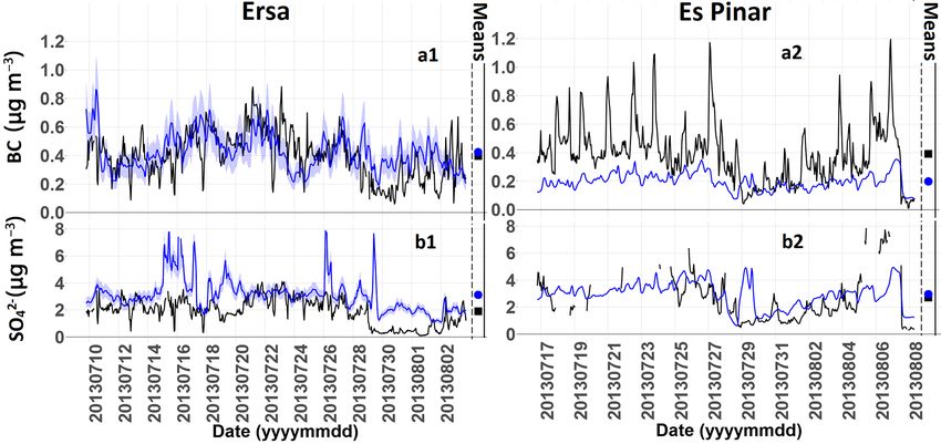
Figure 5. Time series showing the comparison of simulated (in blue) and measured (in black) gaseous species during the
ChArMEx/SAFMED campaign period. (a) Nitrogen oxides (time series in red for Es Pinar represents NOy concentrations); (b) isoprene;
(c) MACR+MVK (methyl vinyl ketone+methacrolein); (d) monoterpenes. Statistical data for these comparisons are given in Table 2. The
ribbon around Ersa simulations presents the orographic representativeness error. On the right side of each time series, two points are shown
presenting the average of simulations (blue circle) and observations (black square).
ety of typical Mediterranean tree and vegetation species mix, graphical characteristics mentioned before for this site, the
that MEGAN correctly simulated (within 10 % error) mean meteorological inputs did not simulate these fog events and
observed monoterpene fluxes over the last 2 weeks of Au- therefore cloud scavenging was not activated in the simula-
gust 2007 for a variety of Mediterranean tree and vegetation tion. Since these decreases concern only a small percentage
species mix, as long as a canopy model was included (as in of the observations, they do not have a major effect on the
our study). outcome of these comparisons. While this effect is very vis-
ible for sulfates, it is less pronounced for other particulate
4.4 Particulate species species such as BC and OA. A large sulfate peak simulated
in the morning of 29 July is not present in the observations; it
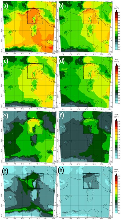
Figure 6 shows the comparison between observations and originates in the model from an air mass arriving from Mar-
simulations for particulate sulfate and BC in PM1 . These two seille, which is both a busy harbor and an important industrial
species are chosen as two important fine aerosol components, area with large SO2 emissions. This is probably due to small
before the comparison of OA in Sect. 5. The left panel shows errors in the wind fields. In addition, there are two periods of
the comparison for Ersa and the right one for Es Pinar. Statis- overestimation of this species in the simulations: the period
tical information for these species is given in Table 4. There of 18 to 20 July and the period of 29 July to the night of 1
is an overestimation for sulfate particles (Fig. 6b1 and b2) by August. During the second period, the ACSM PM1 observa-
about 45 %, well beyond the representativeness error for this tions show concentrations of close to zero, which are consis-
species (15 %). In addition, the short and sharp decreases in tent with PM10 particle-into-liquid sampler ion chromatogra-
the measurements of sulfates correspond to low clouds pass- phy (PILS-IC) sulfate measurements. For this period elevated
ing at the level of the station, which are not simulated by southerly winds are observed in the Corsica area, and the ab-
the model. Cloud scavenging processes are already taken into sence of strong SO2 sources in this sector might explain the
account in the model. However, because of the unique geo- lower concentrations that are seen not only for sulfate but
Atmos. Chem. Phys., 18, 7287–7312, 2018 www.atmos-chem-phys.net/18/7287/2018/You can also read